Abstract

The inclusive distributions of gluons and pions are calculated with absolute normalization for high-energy nucleon-nucleon collisions. The results for several unintegrated gluon distributions from the literature are compared. The gluon distribution proposed recently by Kharzeev and Levin based on the idea of gluon saturation is tested against DIS data from HERA. We find huge differences in both rapidity and transverse momentum distributions of gluons and pions in nucleon-nucleon collisions for different models of unintegrated gluon distributions. The approximations used recently in the literature are discussed. The Karzeev-Levin gluon distribution gives extremely good description of momentum distribution of charged hadrons at midrapidities. Contrary to a recent claim in the literature, we find that the gluonic mechanism discussed does not describe the inclusive spectra of charged particles in the fragmentation region, i.e. in the region of large $|y|$ for any unintegrated gluon distribution from the literature.

1 Introduction

The recent results from RHIC (see e.g. [1]) have attracted renewed interest in better understanding the dynamics of particle production, not only in nuclear collisions.

Quite different approaches [2, 4, 3] have been used to describe the particle spectra from the nuclear collisions [4]. The thermal models do not make a direct link to nucleon-nucleon collisions. In contrast, in dual parton approaches (DPM) the nucleon-nucleon collisions are the basic ingredients of nuclear collisions. Somewhat extreme model in Ref.[3] with an educated guess for unintegrated gluon distribution describes surprisingly well the whole charged particle rapidity distribution by means of gluonic mechanisms only. Such a gluonic mechanism would lead to the identical production of positively and negatively charged hadrons. The recent results of the BRAHMS experiment [5] put into question the successful description of Ref.[3] and show that the DPM type approaches seems more correct. In the light of the BRAHMS experiment is becomes obvious that the large rapidity regions have more complicated flavour structure. The pure gluonic mechanisms, if at all, can be dominant only at midrapidities although the charged kaons [5] show that even this is doubtful. Similarly also the thermal models have difficulties to describe the (pseudo)rapidity dependence of particle to antiparticle ratios [5] and have to limit to the midrapidity only. In principle, the dynamics in nucleus-nucleus collision is fairly complicated and requires a separate analysis. In the following I concentrate only on nucleon-nucleon collisions – the basic ingredients of the nucleus-nucleus collisions.

On the microscopic level the approach of Kharzeev and Levin [3] is based on the gluon-gluon fusion. The gluon-gluon fusion is expected to be the dominant process at midrapidities and at asymptotically large energies. It is not clear how large the energy should be to validate this thesis. The physics in the fragmentation region is somewhat different. It was suggested long ago [6] that pions in the fragmentation region are correlated with the valence quark distributions in hadrons.

The standard hadronization approaches are based rather on the 2 $\rightarrow$ 2 partonic subprocesses which constitute only a part of the dynamics. The perturbative component of these hybrid models has a flavour structure as dictated by the quark/antiquark distributions. On the other hand, the flavour structure of the remaining soft component is not so explicit. Furthermore the partition into ”soft” and ”hard” components is somewhat arbitrary, being to some extend rather an artifact of a natural failure in applying the (2 $\rightarrow$ 2) pQCD at low transverse momenta of hadrons than a clear border of the two regions.

In this paper I discuss the relation between unintegrated gluon distributions in hadrons and the inclusive momentum distribution of particles produced in hadronic collisions. The results obtained with different unintegrated gluon distributions presented recently in the literature are shown and compared. In the present study I limit to the nucleon-nucleon collisions only and leave the nucleus-nucleus collisions for a separate analysis.

2 Photon-nucleon cross section at high energies

It became a standard in recent years to first describe the HERA data and only then to test the resulting gluon distributions in other processes. We try to follow this reasonable methodology also for jet and particle production.

It is known that the LO total $\gamma^{*}N$ cross section can be written in the form

$$\sigma_{tot}^{\gamma^{*}N}=\sum_{q}\int dz\int d^{2}\rho\;|\Psi_{\gamma^{*}\rightarrow q\bar{q}}(Q,z,\rho)|^{2}\cdot\sigma_{(q\bar{q})N}(x,\rho)\;.$$ (1)

In this paper we take the so-called quark-antiquark photon wave function of the perturbative form [7]. As usual, in order to correct the photon wave function for large dipole sizes (nonperturbative region) we introduce an effective quark/antiquark mass ($m_{eff}=m_{0}$). The dipole-nucleon cross section can be parametrized or calculated from the unintegrated gluon distribution

$$\sigma_{(q\bar{q})N}(x,\rho) = \frac{4\pi}{3}\int\frac{d^{2}\kappa_{t}}{\kappa_{t}^{2}}\left[1-\exp(i\vec{\kappa_{t}}\vec{\rho})\right]\alpha_{s}{\cal F}(x,\kappa_{t}^{2})$$ (2)

$$= \frac{4\pi^{2}}{3}\int\frac{d\kappa_{t}^{2}}{\kappa_{t}^{2}}\left[1-J_{0}(\kappa_{t}\rho)\right]\alpha_{s}{\cal F}(x,\kappa_{t}^{2})\;.$$

In the equation above the running coupling constant is fixed constant or is frozen according to an analytic prescription [8]. In the next section we shall compare the dipole-nucleon cross sections calculated from different unintegrated gluon distributions.

3 Unintegrated gluon distributions

Search for the unintegrated gluon distribution in the nucleon was a subject of active both theoretical and phenomenological research in recent years. Still at present the unintegrated gluon distributions are rather poorly known. The main reason of the difficulties is the fact that the unintegrated gluon distribution is a quantity which depends on at least two variables ($x$ and $\kappa^{2}$) in a nontrivial and a priori unknown way. Another difficulty is in an unambiguous separation of perturbative and nonperturbative regions. In general different phenomena test the unintegrated gluon distribution in different corners of the phase space. Therefore it is not surprising that different gluon distributions found in the literature, extracted from the analyses of different phenomena, differ among themselves considerably [9]. In this section I collect and briefly discuss gluon distributions used in the present calculation of the jet and particle production. There are two different conventions of introducing unintegrated gluon distributions in the literature. The resulting quantities are denoted as $f$ (dimenionless quantity) and ${\cal F}$ (with dimension 1/GeV²). We shall keep this notation throughout the present paper.

3.1 BFKL gluon distribution

At very low $x$ the unintegrated gluon distributions are believed to fulfil BFKL equation [10] (see also [11]). After some simplifications [12] the BFKL equation reads

$$-x\frac{\partial f(x,q_{t}^{2})}{\partial x}=\frac{\alpha_{s}N_{c}}{\pi}q_{t}^{2}\int_{0}^{\infty}\frac{dq_{1t}^{2}}{q_{1t}^{2}}\left[\frac{f(x,q_{1t}^{2})-f(x,q_{t}^{2})}{|q_{t}^{2}-q_{1t}^{2}|}+\frac{f(x,q_{t}^{2})}{\sqrt{q_{t}^{4}+4q_{1t}^{4}}}\right]\;.$$ (3)

The homogeneous BFKL equation can be solved numerically [12]. Here in the practical applications we shall use a simple parametrization for the solution [13]

$$f(x,\kappa_{t}^{2})=\frac{C}{x^{\lambda}}\left(\frac{\kappa_{t}^{2}}{q_{0}^{2}}\right)^{1/2}\frac{{\tilde{\phi}}_{0}}{\sqrt{2\pi\lambda^{\prime\prime}\ln(1/x)}}\exp\left[-\frac{\ln^{2}(\kappa_{t}^{2}/{\bar{q}}^{2})}{r2\lambda^{\prime\prime}\ln(1/x)}\right]$$ (4)

In the above expression $\lambda=4{\bar{\alpha}}_{s}\ln 2$, $\lambda^{\prime\prime}$ = 28 ${\bar{\alpha}}_{s}\zeta(3)$, ${\bar{\alpha}}_{s}=3\alpha_{s}/\pi,\zeta(3)$ = 1.202. The remaining parameters were adjusted in [13] to reproduce with a satisfactory accuracy the gluon distribution which was obtained in [12] as the numerical solution of the BFKL equation. It was found that ${\bar{q}}=q_{0}$ = 1, $C{\bar{\phi}_{0}}$ = 1.19 and $r$ = 0.15 [13].

3.2 Golec-Biernat-Wüsthoff gluon distribution

Another parametrization of gluon distribution in the proton can be obtained based on the Golec-Biernat-Wüsthoff parametrization of the dipole-nucleon cross section with parameters fitted to the HERA data [14]. The resulting gluon distribution reads [15]:

$$\alpha_{s}{\cal F}(x,\kappa_{t}^{2})=\frac{3\sigma_{0}}{4\pi^{2}}R_{0}^{2}(x)\kappa_{t}^{2}\exp(-R_{0}^{2}(x)\kappa_{t}^{2})\;,$$ (5)

where

$$R_{0}(x)=\frac{1}{GeV}\left(\frac{x}{x_{0}}\right)^{\lambda/2}\;.$$ (6)

From their fit to the data: $\sigma_{0}$ = 29.12 mb, $x_{0}$ = 0.41 $\cdot$ 10^-4, $\lambda$ = 0.277 [14]. In order to determine the gluon distribution needed in calculating jet and particle production we shall take $\alpha_{s}$ = 0.2.

3.3 Kharzeev-Levin gluon distribution

Another parametrization, also based on the idea of gluon saturation, was proposed recently in [3]. In contrast to the GBW approach [14], where the dipole-nucleon cross section is parametrized, in the Karzeev-Levin approach it is the gluon distribution which is parametrized. In the following we shall consider the most simplified functional form:

$${\cal F}(x,\kappa^{2})=\begin{cases}f_{0}&\text{if}\;\kappa^{2}<Q_{s}^{2},\\ f_{0}\cdot\frac{Q_{s}^{2}}{\kappa^{2}}&\text{if}\;\kappa^{2}>Q_{s}^{2}.\end{cases}$$ (7)

The saturation momentum $Q_{s}$ is parametrized exactly as in the GBW model $Q_{s}^{2}(x)=$ 1 GeV² $\cdot\left(\frac{x_{0}}{x}\right)^{\lambda}$. It was claimed in [3] that the gluon distribution like (7) leads to a good description of the recent RHIC rapidity distributions. It is interesting to check its performance for the deep inelastic scattering at low Bjorken $x$.

In the following the normalization constant $f_{0}$ is adjusted to roughly describe the HERA data. We find $f_{0}$ = 170 mb. The quality of the fit is shown in Fig. 1 for $Q^{2}$ = 0.25, 5, 10 GeV².

Figure 1: The cross section $\sigma_{tot}^{\gamma^{*}p}$ as a function of the center of mass energy $W$ for $Q^{2}$ = 0.25 GeV², $Q^{2}$ = 5 GeV² and $Q^{2}$ = 10 GeV². The results obtained with the KL gluon distribution ($m_{0}$ = 0.15/0.10 GeV) are shown by the solid and dashed lines. Experimental data were taken from [25].

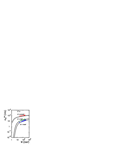
In this fit the running coupling constant frozen according to [8] was used. The result at low photon virtuality ($Q^{2}$ = 0.25 GeV²) depends also on the value of the quark/antiquark effective mass. In the calculation in Fig. 1 $m_{0}$ = 0.15 GeV (solid) and $m_{0}$ = 0.10 GeV (dashed) was used. It can be inferred from the figure that the (virtual) photon-proton cross section at large virtuality ($Q^{2}$ = 5,10 GeV²) is in practice independent of the effective quark mass. This allows to fix the gluon normalization constant $f_{0}$.

In order to better visualize the difference to the GBW model, in Fig. 2 I compare the dipole-nucleon

Figure 2: The dipole-nucleon cross section as a function of the transverse dipole size $\rho$ for the GBW (dashed) and KL (dotted) unintegrated gluon distributions.

cross sections in both parametrizations for $x=10^{-2}$, 10^-3, 10^-4. In the GBW approach the dipole-nucleon cross section saturates at large dipole size. In contrast to the GBW parametrization, the dipole-nucleon cross section calculated according to Eq.(2) based on the KL gluon distribution (7) grows slowly with the dipole size $\rho$.

3.4 Kimber-Martin-Ryskin gluon distribution

The unintegrated gluon distribution can be obtained even when the integrated gluon distribution fulfils standard DGLAP evolution equation. At very small $x$

$${\cal F}(x,\kappa^{2})=\frac{\partial}{\partial Q^{2}}\left[xg(x,Q^{2})\right]|_{Q^{2}=\kappa^{2}}\;.$$ (8)

This prescription breaks at larger values of $x$ when the derivative of the gluon distribution becomes negative. This may be somewhat improved by introducing a Sudakov form factor $T_{g}(\kappa^{2},\mu^{2})$. Then the unintegrated gluon distribution reads [18]:

$${\cal F}(x,\kappa^{2},\mu^{2})=\frac{\partial}{\partial Q^{2}}\left[T(Q^{2},\mu^{2})xg(x,Q^{2})\right]|_{Q^{2}=\kappa^{2}}\;.$$ (9)

Resumming virtual contributions to DGLAP equation, the unintegrated parton distributions can be written as [18]

$$f_{a}(x,\kappa^{2},\mu^{2})=T_{a}(\kappa^{2},\mu^{2})\cdot\frac{\alpha_{s}(\kappa^{2})}{2\pi}\sum_{a^{\prime}}\int_{x}^{1-\delta}P_{aa^{\prime}}(z)\left(\frac{x}{z}\right)a^{\prime}\left(\frac{x}{z},\kappa^{2}\right)dz\;.$$ (10)

Specializing to the gluon distribution the Sudakov form factor reads as

$$T_{g}(\kappa^{2},\mu^{2})=\exp\left(-\int_{\kappa^{2}}^{\mu^{2}}\frac{dp^{2}}{p^{2}}\frac{\alpha_{s}(p^{2})}{2\pi}\int_{0}^{1-\delta}dzz\left[P_{gg}(z)+\sum_{q}P_{qg}(z)\right]\right)\;.$$ (11)

The Sudakov form factor introduces a dependence on a second scale $\mu^{2}$. It is reasonable to assume that the unintegrated gluon density given by (10) starts only for $\kappa_{t}^{2}>\kappa_{t0}^{2}$ [16]. At lower $\kappa_{t}^{2}$ an extrapolation is needed. In our case of particle distributions the results are sensitive to rather low $\kappa$. Because of this, a use of the GRV integrated gluon distribution [19, 20] in (10) seems more adequate than any other PDF. Following Ref.[17] $\kappa_{t0}^{2}$ = 0.5 GeV² is taken as the lowest value where the unintegrated gluon distribution is calculated from Eq.(10). Below it is assumed

$${\cal F}(x,\kappa^{2})=f(x,\kappa^{2})/\kappa^{2}=f(x,\kappa_{0}^{2})/\kappa_{0}^{2}\;.$$ (12)

The choice of $\mu^{2}$ in our case of jet (particle) production is not completely obvious. In the present analysis $\mu^{2}=p_{t}^{2}$ is assumed, where $p_{t}$ is transverse momentum of the produced gluon ($\equiv$ jet). In accord with the interpretation of the Sudakov form factor as a survival probability we assume that if transverse momentum of the produced gluon is smaller than the transverse momentum of the last gluon of the ladder ($p_{t}<\kappa_{1}$ or $p_{t}<\kappa_{2}$, see next section) then the corresponding Sudakov form factor is set to 1, i.e. we do not allow for any enhancement. If $T_{g}$ in Eq.(10) is ignored we shall denote the corresponding gluon distribution as $f_{DGLAP}$ or ${\cal F}_{DGLAP}$ and call it DGLAP gluon distribution for brevity.

3.5 Blümlein gluon distribution

In the approach of Blümlein [21] the $\kappa_{t}^{2}$ dependent gluon distribution satisfying the BFKL equation can be represented as the convolution of the integrated gluon density $xg(x,\mu^{2})$ and a universal function $\cal{B}$

$${\cal F}(x,\kappa_{t}^{2},\mu^{2})=\int_{x}^{1}{\cal B}(z,\kappa_{t}^{2},\mu^{2})\frac{x}{z}g(\frac{x}{z},\mu^{2})dz\;.$$ (13)

The universal function ${\cal B}(x,\kappa_{t}^{2},\mu^{2})$ can be represented as a series [21]. The first term of the expansion describes BFKL dynamics in the double-logarithmic approximation:

$${\cal B}(z,\kappa_{t}^{2},\mu^{2})=\begin{cases}\frac{{\bar{\alpha}}_{s}}{z\kappa_{t}^{2}}J_{0}(2\sqrt{{\bar{\alpha}_{s}}\log(1/z)\log(\mu^{2}/\kappa_{t}^{2})})&\text{if}\;\kappa_{t}^{2}<\mu^{2}\\ \frac{{\bar{\alpha}}_{s}}{z\kappa_{t}^{2}}I_{0}(2\sqrt{{\bar{\alpha}_{s}}\log(1/z)\log(\kappa_{t}^{2}/\mu^{2})})&\text{if}\;\kappa_{t}^{2}>\mu^{2},\end{cases}$$ (14)

where ${\bar{\alpha}_{s}}=3\alpha_{s}/\pi$.

In DIS there is a natural choice of the scale $\mu^{2}$. The choice of the scale is not so obvious in the case considered in the present paper. I shall argue that in practice the dependence on that scale is very weak. In the following I shall use the integrated gluon distribution in Eq.(13) from Ref. [19].

4 Inclusive gluon production

Before we go to particle production in the next section, let us consider the first step of the process – production of partons. At high energies gluons are the most abundantly produced partons in hadron-hadron collisions. Also gluons are responsible for their production.

At sufficiently high energy the cross section for inclusive gluon production in $h_{1}+h_{2}\rightarrow g$ can be written in terms of the unintegrated gluon distributions “in” both colliding hadrons:

$$\frac{d\sigma}{dyd^{2}p_{t}}=\frac{16N_{c}}{N_{c}^{2}-1}\frac{1}{p_{t}^{2}}\int\alpha_{s}(\Omega^{2}){\cal F}_{1}(x_{1},\kappa_{1}^{2}){\cal F}_{2}(x_{2},\kappa_{2}^{2})\delta(\vec{\kappa}_{1}+\vec{\kappa}_{2}-\vec{p}_{t})\;d^{2}\kappa_{1}d^{2}\kappa_{2}\;.$$ (15)

In the equation above $f_{1}$ and $f_{2}$ are unintegrated gluon distributions in hadron $h_{1}$ and $h_{2}$, respectively. The longitudinal momentum fractions are fixed by kinematics: $x_{1/2}=\frac{p_{t}}{\sqrt{s}}\cdot\exp(\pm y)$. Generally the smaller jet (parton) momenta $p_{t}$, the smaller $x_{1/2}$ come into play. The argument of the running coupling constant is taken as $\Omega^{2}=\max(\kappa_{1}^{2},\kappa_{2}^{2},p_{t}^{2})$. The formula (15) above was first written by Gribov, Levin and Ryskin [22] (see also [23]) and used later e.g. in [13]. As discussed in Ref.[24] the normalization of the cross section in some previous works was not always correct. Making use of the $\delta$ function (momentum conservation) one can simplify (15) to the integral

$$\frac{d\sigma}{dyd^{2}p_{t}}=\frac{16N_{c}}{N_{c}^{2}-1}\frac{1}{p_{t}^{2}}{\frac{1}{4}}\int\alpha_{s}(\Omega^{2}){\cal F}_{1}\left(x_{1},\left(\frac{\vec{p}_{t}+\vec{q}_{t}}{2}\right)\right){\cal F}_{2}\left(x_{2},\left(\frac{\vec{p}_{t}-\vec{q}_{t}}{2}\right)\right)d^{2}q_{t}\;,$$ (16)

where $\vec{q}_{t}=\vec{\kappa}_{1}-\vec{\kappa}_{2}$ was introduced. The factor 1/4 is the jacobian of transformation from ($\vec{\kappa}_{1}$, $\vec{\kappa}_{2}$) to ($\vec{p}_{t}$, $\vec{q}_{t}$). The integral above is a two-dimensional integral over $d^{2}q_{t}$, i.e. over $q_{t}dq_{t}d\phi$, where $\phi$ is the azimuthal angle between $q_{t}$ and $p_{t}$. The original integral (16) can be written as

$$\frac{d\sigma}{dyd^{2}p_{t}}=\int\;I(\phi)\;d\phi\;,$$ (17)

where

$$I(\phi)=\frac{4N_{c}}{N_{c}^{2}-1}\frac{1}{p_{t}^{2}}\int\alpha_{s}(\Omega^{2}){\cal F}_{1}\left(x_{1},\kappa_{1}^{2}\right){\cal F}_{2}\left(x_{2},\kappa_{2}^{2}\right)\;q_{t}dq_{t}\;.$$ (18)

Figure 3: The intrinsic azimuthal correlations for different unintegrated gluon distributions: GBW (dashed), KL (solid), BFKL (dotted), Blümlein (thick dash-dotted), DGLAP (thick dashed) and KMR (thick solid) at W = 200 GeV.

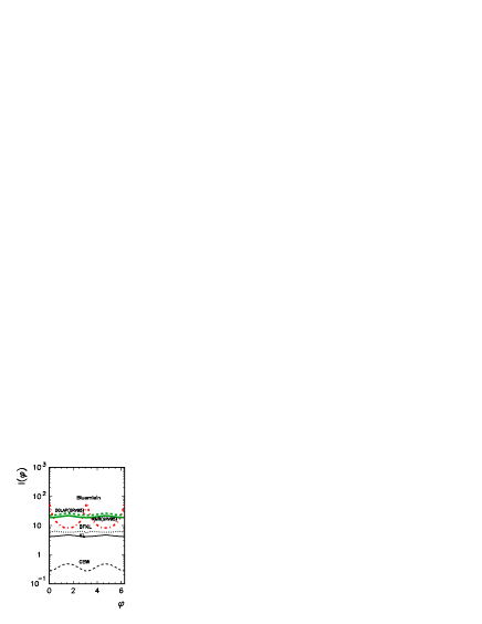
In Fig. 3, I show the intrinsic angular correlation function $I(\phi)$ for different models of unintegrated gluon distributions for a RHIC energy $W$ = 200 GeV. In this calculation y=0 and $p_{t}$ = 1 GeV was taken. Quite a different pattern is obtained for different unintegrated gluon distributions. The $\phi$-distribution is flat for the KL, BFKL, DGLAP and KMR gluon distributions. The most pronounced structure is obtained with the Blümlein gluon distribution [21](GRV95, $\mu^{2}$ = 10 GeV²). It was checked that the Blümlein (GRV95) gluon distribution is not very sensitive to the choice of the second scale $\mu^{2}$. The $\phi$ dependence at $y\neq$ 0 also strongly depends on the unintegrated gluon distribution.

It was suggested in [3] that the integral (16) may be approximated by the formula

$$\frac{d\sigma}{dyd^{2}p_{t}}=\frac{4N_{c}\alpha_{s}}{N_{c}^{2}-1}\frac{1}{p_{t}^{2}}\int\left[{\cal F}_{1}(x_{1},{p}_{t}^{2}){\cal F}_{2}(x_{2},{q}_{t}^{2})+{\cal F}_{1}(x_{1},{q}_{t}^{2}){\cal F}_{2}(x_{2},{p}_{t}^{2})\right]dq_{t}^{2}\;.$$ (19)

Figure 4: A comparison of the gluon rapidity distributions obtained from the exact (16) (thick lines) and approximate (19) (thin lines) formula for different models of unintegrated gluon distributions at W = 200 GeV.

Figure 5: A comparison of the gluon transverse momentum distributions obtained from the exact (16) (thick lines) and approximate (19) (thin lines) formula for different models of unintegrated gluon distributions at W = 200 GeV.

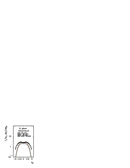
In Fig.4 (rapidity distribution) and Fig.5 (transverse momentum distribution) I compare the results using the exact Eq.(16) and the approximate Eq.(19) formulae for different models of unintegrated gluon distributions. In Fig.4 the integration over $p_{t}>$ 0.5 GeV is performed while in Fig.5 -1 $<y<$ 1. In both cases $\alpha_{s}$ was fixed at 0.2. As can be seen by inspection of the figures the use of the approximate formula is quantitatively justified for the KL, BFKL gluon distributions and not justified for the GBW one.

Figure 6: Inclusive gluon rapidity distribution ($p_{t}>$ 0.5 GeV) at W = 200 GeV for different models of unintegrated gluon distributions.

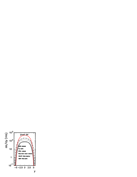
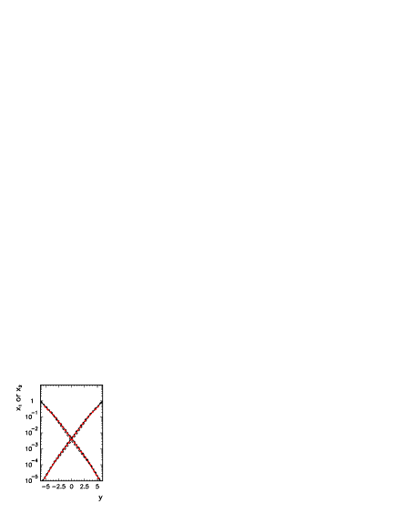
In Fig.6 I compare the cross section $\frac{d\sigma}{dy}(y)$ for different models of unintegrated gluon distributions. In this calculation $p_{t}<$ 0.5 was assumed. The rapidity distribution of gluons are rather different for different gluon PDF. Average values of $x_{1}$ and $x_{2}$ obtained with different gluon distribution with the $p_{t}$ interval chosen are shown in Fig.7. The following general observations can be made. Average value $<x_{1}>$ and $<x_{2}>$ only weakly depend on the model of unintegrated gluon distribution. For $y\sim$ 0 at the RHIC energy W = 200 GeV one tests unintegrated gluon distributions at $x_{g}$ = 10^-3 - 10^-2. This is the region known already from the HERA kinematics. When $|y|$ grows one tests more and more asymmetric (in $x_{1}$ and $x_{2}$) configurations. For large $|y|$ either $x_{1}$ is extremely small ($x_{1}<$ 10^-4) and $x_{2}\rightarrow$ 1 or $x_{1}\rightarrow$ 1 and $x_{2}$ is extremely small ($x_{2}<$ 10^-4). These are regions of gluon momentum fraction where the unintegrated gluon PDF is rather poorly known. The approximation used in obtaining unintegrated gluon distributions are valid certainly only for $x<$ 0.1. In order to extrapolate the gluon distribution to $x_{g}\rightarrow$ 1 I multiply the gluon distributions from the previous section by a factor $(1-x_{g})^{n}$, where n = 5-7.

Figure 7: The average value of $x_{1}$ and $x_{2}$ for $p_{t}>$ 0.5 GeV and at W = 200 GeV. Lines corresponding to different unintegrated gluon PDF are identical as in the previous figure.

In the approach considered in the present paper (for details see next section) the production of particles is sensitive to rather small gluon (called equivalently jet despite of the small transverse momentum) transverse momenta.

Figure 8: Inclusive gluon transverse momentum distribution (-1 $<y<$ 1) at W = 200 GeV for different models of unintegrated gluon distributions: BFKL (dotted), GBW (dashed), KL (solid), Blümlein (thick dash-dotted) and DGLAP (thick dashed).

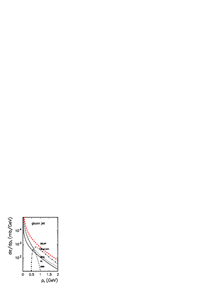
In Fig.8 I plot $\frac{d\sigma}{dp_{t}}(p_{t})$ in the low $p_{t}$ region. In these calculations the gluon rapidity was integrated in the interval -1 $<y<$ 1. The results obtained with different models for unintegrated gluon distributions differ considerably. The transverse momentum distribution obtained with the GBW gluon density is much steeper than the distribution for any other gluon density. The inclusion of DGLAP evolution as in [26] would probably change the situation. In the case of the Blümlein gluon distribution the transverse momentum spectrum has a natural low-$p_{t}$ cut-off if the scale $\mu^{2}=p_{t}^{2}$ is chosen. If similar prescription of the scale is used for calculating gluon transverse momentum distribution with KMR method the DGLAP and KMR results are almost identical. Contrary to the claim in [3] the result obtained with the GBW and KL gluon distributions differ considerably.

The rapidity and pseudorapidity distributions of partons (massless particles) are identical. The situation changes when massive particles are produced in the final state via fragmentation. Below we discuss how to take into account the unknown hadronization process with the help of phenomenological fragmentation functions.

5 From gluon to particle distributions

In Ref.[3] it was assumed, based on the concept of local parton-hadron duality, that the rapidity distribution of particles is identical to the rapidity distribution of gluons. This seems to be a very severe assumption and for massive particles this idea must lead to incorrect results, especially in the fragmentation region. This approach leads to e.g. (massive) particles with rapidities ($y_{h}$) beyond the allowed kinematical region ($y_{h,min},y_{h,max}$). Furthermore in [3] the normalization of rapidity distributions was fitted to the experimental charged particle rapidity distributions. In our opinion, the good description of the charged particle distribution in the full range of rapidity in Ref. [3] is due to these simplifications rather than due to the underlying dynamics.

In the present approach I follow a different, yet simple, approach which makes use of phenomenological fragmentation functions (see e.g.[27, 28]). For our present exploratory study it seems sufficient to assume that the emitted hadron, mostly pion, is collinear to the gluon direction ($\theta_{h}=\theta_{g}$). This is equivalent to $\eta_{h}=\eta_{g}=y_{g}$, where $\eta_{h}$ and $\eta_{g}$ are hadron and gluon pseudorapitity, respectively.

In experiments a good identification of particles is not always achieved which makes impossible to determine the rapidity of a particle. The practice then is to measure pseudorapidity. The rapidity of a given type of hadrons ($y_{h}$) with a mass $m_{h}$ can be obtained from the pseudorapidity as

$$y_{h}=\frac{1}{2}\left[\frac{\sqrt{\frac{m_{h}^{2}+p_{t,h}^{2}}{p_{t,h}^{2}}+\sinh^{2}\eta_{h}}+\sinh\eta_{h}}{\sqrt{\frac{m_{h}^{2}+p_{t,h}^{2}}{p_{t,h}^{2}}+\sinh^{2}\eta_{h}}-\sinh\eta_{h}}\right]\;.$$ (20)

The collinearity of partons and particles leads to the following relation between rapidity of the gluon and hadron

$$y_{g}=\mathrm{arsinh}\left(\frac{m_{t,h}}{p_{t,h}}\sinh y_{h}\right)\;,$$ (21)

where the transverse mass $m_{t,h}=\sqrt{m_{h}^{2}+p_{t,h}^{2}}$. In order to introduce phenomenological fragmentation functions one has to define a new kinematical variable. In accord with $e^{+}e^{-}$ and $ep$ collisions I define a standard auxiliary quantity $z$ by the equation $E_{h}=zE_{g}$. This leads to the following relation between transverse momenta of the gluon and hadron

$$p_{t,g}=\frac{p_{t,h}}{z}J(m_{t,h},y_{h})\;,$$ (22)

where

$$J(m_{t,h},y_{h})=\left(1-\frac{m_{h}^{2}}{m_{t,h}^{2}\cosh^{2}y_{h}}\right)^{-1/2}\;.$$ (23)

Now we can write the single particle distribution in terms of the gluon distribution from the last section as follows

$$\frac{d\sigma(\eta_{h},p_{t,h})}{d\eta_{h}d^{2}p_{t,h}}=\int dy_{g}d^{2}p_{t,g}\int dz\;D_{g\rightarrow h}(z,\mu_{D}^{2})$$ (24)

$$\delta(y_{g}-\eta_{h})\;\delta^{2}\left(\vec{p}_{t,h}-\frac{z\vec{p}_{t,g}}{J}\right)\cdot\frac{d\sigma(y_{g},p_{t,g})}{dy_{g}d^{2}p_{t,g}}\;.$$

Making use of the $\delta$ functions we can write the single particle spectrum as

$$\frac{d\sigma(\eta_{h},p_{t,h})}{d\eta_{h}d^{2}p_{t,h}}=\int_{z_{min}}^{z_{max}}dz\frac{J^{2}D_{g\rightarrow h}(z,\mu_{D}^{2})}{z^{2}}\frac{d\sigma(y_{g},p_{t,g})}{dy_{g}d^{2}p_{t,g}}\Bigg{|}_{y_{g}=\eta_{h}\atop p_{t,g}=Jp_{t,h}/z}\;.$$ (25)

Experimentally instead of the two-dimensional spectrum (25) one determines rather one-dimensional spectra in either $\eta_{h}$ or $p_{t,h}$.

The one-dimensional pseudorapidity distribution can be obtained by integration over hadron transverse momenta

$$\frac{d\sigma(\eta_{h})}{d\eta_{h}}=\int d^{2}p_{t,h}\;\frac{d\sigma(\eta_{h},p_{t,h})}{d\eta_{h}d^{2}p_{t,h}}\;.$$ (26)

Figure 9: Charged-pion pseudorapidity distribution at W = 200 GeV for the KL unintegrated gluon distribution for different parametrizations of fragmentation functions. In this calculation $p_{t,h}>$ 0.2 GeV. The experimental data of the UA5 collaboration are taken from [35].

Stable particles are produced directly in the fragmentation process or are decay products of other unstable particles. There are a few global analyses of fragmentation function in the literature up to next-to-leading order [30, 31, 32, 33]. In the present calculation I shall use only leading order fragmentation functions from [30, 31]. One should remember, however, that both $e^{+}e^{-}$ and $ep$ collisions do not allow to uniquely determine $D_{g\rightarrow h}$ fragmentation functions. In order to test sensitivity of our results to these, in my opinion, not quite well known objects I shall use also simple functional forms: $D_{g\rightarrow h}(z)=2\frac{1-z}{z}$ (model I) or $D_{g\rightarrow h}(z)=3\frac{(1-z)^{2}}{z}$ (model II) with the factors in front adjusted to conserve momentum sum rule. When charged particles are measured only, then to a good approximation it is sufficient to multiply the fragmentation functions above by a factor 2/3.

Figure 10: Charged-pion pseudrapidity distribution at W = 200 GeV for different models of unintegrated gluon distributions. In this calculation $p_{t,h}>$ 0.2 GeV. The experimental data of the UA5 collaboration are taken from [35].

In Fig.9 I compare pseudorapidity distribution of charged pions at W = 200 GeV calculated with the KL gluon distribution and different parametrizations of fragmentation functions. For the BKK1995 [30] and for the KKP2000 [31] fragmentation functions the factorization scale was set to $\mu_{D}^{2}=p_{t,g}^{2}$, except for $p_{t,g}<$ 1 GeV, where it was frozen at $\mu_{D}^{2}=$ 1 GeV². For reference shown are also experimental data for charged particles measured by the UA5 collaboration at CERN [35]. The results only weakly depend on the choice of the $g\rightarrow\pi$ fragmentation function. It is worth stressing that the theoretical cross section at $\eta_{h}\approx$ 0 is almost consistent with the experimental one. However, the shapes of theoretical and experimental pseudorapidity distributions differ significantly. It seems there is a room for different mechanisms typical for fragmentation regions. The specificity of these regions will be discussed elsewhere.

Let us analyze now how the results for pseudorapidity distributions depend on the choice of the unintegrated gluon distribution. In Fig.10 I compare pseudorapidity distribution of charged pions for different models of unintegrated gluon distributions. In this calculation the Binnewies-Kniehl-Kramer fragmentation function [30] has been used. The conclusions inferred above stay true also here. Having in view a dramatically steep $p_{t,g}$ distribution in Fig.8 it is rather surprising that the normalization of the spectra at midrapidities comes roughly correct, although very is a tendency to an overestimation for some gluon distributions. This can be due to the fit to DIS data, where the resolved photon component has been neglected. If the resolved photon component is explicitly included [34] then the normalization of the dipole-nucleon component (dipole-nucleon cross section or unintegrated gluon distribution) must be reduced.

Figure 11: Average values of $\left<p_{t}^{2}\right>$ (solid), $\left<\kappa_{1}^{2}\right>$ (dashed) and $\left<\kappa_{2}^{2}\right>$ (dotted) as a function of pion pseudorapidity

What are typical transverse momenta of gluons involved in the calculations is shown in Fig.11. In this calculation we have used the KL unintegrated gluon distribution and the BKK $g\rightarrow\pi$ fragmentation functions [30]. We observe a maximum of the transverse momentum squared of the produced gluon at $\eta_{h}\approx$ 0. In our implementation of fragmentation ($p_{t,h}^{2}\ll p_{t,g}^{2}$) one tests relatively large $p_{t,g}^{2}$. While at midrapidities $\left<p_{t}^{2}\right>>\left<\kappa_{1}^{2}\right>,\left<\kappa_{2}^{2}\right>$, when going to the fragmentation regions the relation reverses. In the whole range of pseudorapidity one tests on average $\kappa_{1}^{2},\kappa_{2}^{2}\sim$ 1 GeV². One should remember, however, that at the same time $\left<x_{1}\right>$ and $\left<x_{2}\right>$ change dramatically when going from midrapidities to the fragmentation region.

Figure 12: The pseudorapidity distribution of protons (solid), antiprotons (dashed) and the difference of the spectra of $\pi^{+}$ and $\pi^{-}$ (dash-dotted) in the proton-proton collision at W = 200 GeV obtained with the code HIJING [37]. The thick solid line corresponds to the sum of these three contributions. The experimental data of the UA5 collaboration are taken from [35].

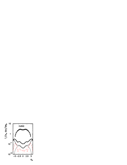
In contrast to Ref.[3], where the whole pseudorapidity distribution, including fragmentation regions, has been well described in an approach similar to the one presented here, in the present paper pions produced from the fragmentation of gluons in the $gg\rightarrow g$ mechanism populate only midrapidity region, leaving room for other mechanisms in the fragmentation regions. These mechanisms involve quark/antiquark degrees of freedom or leading protons among others. In Fig.12 I show the pseudorapidity spectra of protons, antiprotons and the difference $d\sigma/d\eta_{\pi^{+}}-d\sigma/d\eta_{\pi^{-}}$ obtained with the code HIJING [37] (see also [38]). The difference of the proton-antiproton spectra gives an idea of leading particle contribution. Both protons from deeply inelastic events as well as protons from diffraction dissociation (single diffraction) have been included. The difference of the positively and negatively charged pions gives the lower limit on the $\pi^{+}-\pi^{-}$ asymmetric mechanisms not taken into account in the Kharzeev-Levin approach. The sum of the three contributions (thick solid) gives then lower limit on the missing contributions. It is of the similar size as the missing contributions in Fig.9 and Fig.10. This strongly suggests that the agreement of the result of the $gg\rightarrow g$ approach with the PHOBOS distributions [4] in Ref.[3] in the true fragmentation region is rather due to approximations made in [3] than due to correctness of the reaction mechanism. In principle, this can be verified experimentally at RHIC by measuring the $\pi^{+}/\pi^{-}$ ratio in proton-proton scattering as a function of (pseudo)rapidity in possibly broad range. It seems that the BRAHMS experiment, for instance, can do it even with the existing apparatus.

Figure 13: Transverse momentum distributions of charged pions at W = 200 GeV for the KL gluon distribution and different fragmentation functions. The experimental data of the UA1 collaboration are taken from [36].

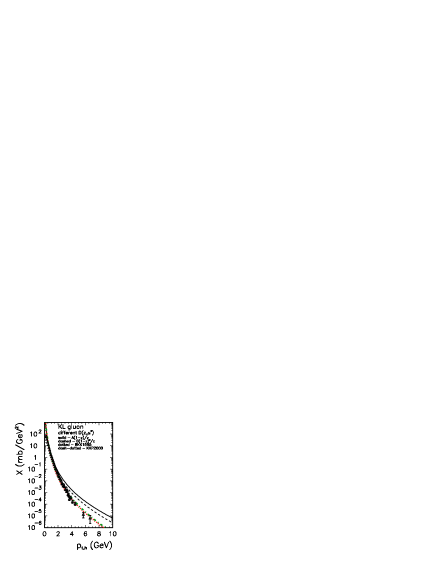
The transverse momentum distribution of charged hadrons is shown in Fig.13 together with experimental data of the UA1 collaboration at CERN from Ref.[36]. In this calculation the KL gluon distribution has been used. It is not completely clear to me how the experimental data in [36] should be interpreted. I assume that the experimental data should be interpreted as:

$$X=\int\frac{d\sigma}{d\eta_{h}d^{2}p_{t}}d\eta_{h}\;/\;\int d\eta_{h}\;.$$ (27)

We have taken $\eta_{h}\in$ (-2.5,2.5). The simple hadronization functions, called model I and II above, correctly fit low $p_{t,h}$ data and fail in the large $p_{t,h}$ region. This is due to lack of QCD evolution [29]. The results obtained with fragmentation functions from [30, 31] which include DGLAP evolution, extremely well describe the large $p_{t,h}$ data. Having in mind the ambiguity of the experimental data interpretation, the KL gluon distribution does a fairly good job.

In Fig.14 I compare the theoretical transverse momentum distributions of charged pions obtained with different gluon distributions with the UA1 collaboration data [36]. The best agreement is obtained with the Karzeev-Levin gluon distribution. The distribution with the GBW model is much too steep in comparison to experimental data. This is probably due to neglecting QCD evolution.

Figure 14: Transverse momentum distributions of charged pions at W = 200 GeV for BKK1995 fragmentation function and different models of unintegrated gluon distributions. The experimental data of the UA1 collaboration are taken from [36].

6 Conclusions

I have calculated the inclusive distributions of gluons and associated charged pions in the nucleon-nucleon collisions through the $gg\rightarrow g$ mechanism in the $k_{t}$-factorization approach. The results for several unintegrated gluon distributions proposed recently in the literature have been compared. The results, especially transverse momentum distributions, obtained with different models of unintegrated gluon distributions differ considerably.

A special attention has been devoted to the gluon distribution proposed recently by Kharzeev and Levin to describe charged particle production in relativistic heavy-ion collisions. In the first step I have tested the gluon distribution in electron deep-inelastic scattering at small Bjorken $x$. A rather good description of the HERA data can be obtained by adjusting a normalization constant. In the next step so-fixed gluon distribution has been used to calculate (pseudo)rapidity and transverse momentum distribution of gluonic jets and charged particles.

Huge differences in both rapidity and transverse momentum distributions of gluons and pions for different models of unintegrated gluon distributions have been found.

Some approximations used recently in the literature have been discussed. Contrary to a recent claim in Ref.[3], we have found that the gluonic mechanism discussed does not describe the inclusive spectra of charged particles in the fragmentation region, i.e. in the region of large (pseudo)rapidities for any unintegrated gluon distribution from the literature. Clearly the gluonic mechanism is not the only one and other mechanisms (see e.g.[27, 28] ) neglected in [3] must be added. Some of them have been estimated with the help of the HIJING code, giving a right order of magnitude for the missing strength.

Since the mechanism considered is not complete, it is not possible at present to precisely verify different models of unintegrated gluon distributions. The existing gluon distributions lead to the contributions which almost exhaust the strength at midrapidities and leave room for other mechanisms in the fragmentation regions. It seems that a measurement of transverse momentum distributions of particles at RHIC should be helpful to test better different unintegrated gluon distributions. A good identification of particles is required to verify the other mechanisms.

In contrast to standard integrated gluon distributions, the extraction of unintegrated gluon distribution from experimental data seems a rather difficult task. At present, one can rather test different unintegrated gluon distributions based on different models existing in the literature. In the present analysis I have discussed whether the production of particles can provide some information on unintegrated gluon distributions in the nucleon. There are many other reactions where this is possible, to mention here only heavy quark or jet production in $ep$ and $pp$ collisions. Going to more exclusive measurements seems indispensable. An example is a careful study of jet correlation in photon-proton [39] and nucleon-nucleon [40] collisions. In my opinion, we are at the beginning of the long way to extract gluon or more generally parton unintegrated distributions.

Acknowledgements I am indebted to Jan Kwieciński for several discussions on different subjects concerning high-energy physics, for his willingness to share his knowledge, for his optimism and friendly attitude. The discussion with Andrzej Budzanowski is kindly acknowledged. The pseudorapidity distributions of particles from the code HIJING have been obtained from Piotr Pawłowski. I thank Leszek Motyka for providing me with some FORTRAN routines.