What exactly is a parton density?

Abstract

I give an account of the definitions of parton densities, both the conventional ones, integrated over parton transverse momentum, and unintegrated transverse-momentum-dependent densities. The aim is to get a precise and correct definition of a parton density as the target expectation value of a suitable quantum mechanical operator, so that a clear connection to non-perturbative QCD is provided. Starting from the intuitive ideas in the parton model that predate QCD, we will see how the simplest operator definitions suffer from divergences. Corrections to the definition are needed to eliminate the divergences. An improved definition of unintegrated parton densities is proposed.

12.39.St, 12.38.Aw, 12.38.Bx

1 Introduction

Central to many of the phenomenological applications of QCD are parton densities (or parton distribution functions — pdf’s). The reasons are quite easy to understand, since the primary tool for making scattering calculations in quantum field theories is weak coupling perturbation theory. Because QCD is a theory of the strong interaction, simple fixed-order perturbation theory is useless for almost all physical cross sections and amplitudes. But when a suitable large momentum scale $Q$ is present, we appeal to factorization theorems to separate the momentum and distance scales in a reaction. The asymptotic freedom of QCD then allows us to use low-order perturbation theory in powers of $\alpha_{s}(Q)$ to estimate the short-distance parts of cross sections.

Pdf’s (and related quantities, like fragmentation functions, parton distribution amplitudes, and generalized parton densities) contain the non-perturbative parts of the physics. Because they are universal, the same pdf’s appear in all reactions. They can be measured in a limited set of reactions and then perturbative calculations of hard scattering and pdf evolution enable us to predict, from first principles, cross sections for many other processes. The successes of this formalism are well-known.

A simple example is the factorization theorem for a deep-inelastic structure function:

$$F_{1}(x,Q^{2})=\sum_{i}\int_{x}^{1}\frac{d\xi}{\xi}C_{1i}(x/\xi,Q^{2}/\mu^{2},\alpha_{s}(\mu))\,f_{i}(\xi,\mu),$$ (1)

valid up to power-law corrections at high $Q$. The standard lowest order calculation gives $C_{1i}=\frac{1}{2}e_{i}^{2}\delta(x/\xi-1)$.

Although QCD and factorization appear to form a mature field, the concepts of parton densities and factorization as presented in much of the literature are quite problematic. In fact, as we will see in Sec. 2, many of the definitions of pdf’s in the literature, if taken literally, are wrong. This should be, and often is, confusing to students of the subject, even though solutions to the problems are often well known to experts. Let us just take this as a symptom of the difficulty of our subject, that of making first principles predictions from a strongly interacting, relativistic, quantum many-body theory.

To improve this situation, to make the concepts precise, is particularly important given the central role that calculations based on factorization theorems play in extracting physics consequences from data in high-energy experiments. Furthermore, as searches for new physics get more sophisticated, elaborations of the QCD factorization theorems are needed. For example, Monte-Carlo event generators are commonly used to estimate exclusive components of inclusive cross sections. They are generally considered to be theoretically based on the factorization theorem. But because a detailed and exact treatment of parton kinematics is needed, some kind of unintegrated pdf is needed if the conceptual foundation is to be sound.

In addition, definitions of parton densities form an important link between treatments of non-perturbative bound states in QCD and their application, via factorization theorems, to measurable scattering cross sections. For this link to work, the definitions must be correct.

For issues that are not given specific references, the reader can refer to standard references, for example the book by Ellis, Stirling and Webber [1], the review of factorization theorems by Collins, Soper and Sterman [2], and the CTEQ handbook [3].

2 Development of definitions of pdf’s

2.1 Parton model

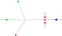
The basic ideas of pdf’s and the parton model are due to Feynman [4] and predate QCD. Consider deep-inelastic scattering (DIS) in the $e$–$p$ center-of-mass frame — Fig. 1. An electron arrives from the left and undergoes a wide-angle scattering. A highly time-dilated and Lorentz contracted proton arrives from the right; it is symbolized by the squashed blob with 3 dots inside (for the valence quarks). For numerical illustration, suppose that $Q^{2}=10^{4}\,\textrm{GeV}^{2}$ and $x=0.5$ at the HERA energy, $\sqrt{s}\simeq 300\,\textrm{GeV}$. The hard interaction occurs with one constituent over a scale $1/Q$, about $0.01\,\textrm{fm}$. In contrast the transverse size of the proton is about $1\,\textrm{fm}$.

Figure 1: Deep-inelastic scattering.

The parton model starts from the reasonable supposition that the interactions binding quarks occur on a time scale $1\,\textrm{fm}/c$ in the rest frame of the proton, and that these get time dilated in the center-of-mass frame, to about $100\,\textrm{fm}/c$ under the above conditions. This suggests that during the interaction of the electron with the hadronic system, it is a useful approximation to assume that the electron interacts with a single fast-moving constituent, or parton, of the proton, and to neglect the strong interactions of the parton with the rest of the proton. That is, the incoming parton is approximated as a free particle for the purposes of calculating the interaction with the electron.

Of course, we know that this approximation and the arguments leading to it are not exactly correct in QCD and other quantum field theories. Even so, the argument contains a core of truth, and it leads to the following formula for the structure functions

$$2xF_{1}(x,Q^{2})=F_{2}(x,Q^{2})=\sum_{i}e_{i}^{2}xf_{i}(x)+O(\alpha_{s}(Q)),$$ (2)

where I have indicated the order of magnitude of the known QCD corrections (different for $2xF_{1}$ and $F_{2}$, of course).

At this level, the pdf $f_{i}(x)$ is informally defined as the single particle density of a parton of fractional momentum $x$ and flavor $i$ in a fast moving hadron. The parton-model formula agrees with the correct factorization result in QCD when the hard-scattering coefficient is given its lowest-order approximation and the DGLAP-evolved pdf’s are evaluated at a scale of order $Q$.

2.2 Light-front quantization

(a)

(b)

Figure 2: (a) Handbag diagram for DIS. (b) Structure of general leading region for DIS. The upper blob has lines with large transverse momentum, and the lower blob has lines with low transverse momentum.

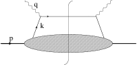
Further progress was made by Bouchiat, Fayet and Meyer [5] and Soper [6, 7]. They observed that the parton model can be implemented in field theory if one assumes that the dominant contributions have the form of the “handbag diagram” of Fig. 2(a), and that the intermediate quark has limited transverse momentum and virtuality. A definition of quark pdf’s results that can be readily interpreted when light-front quantization is used to define annihilation and creation operators $a_{i}(k^{+},\bm{k}_{T},\lambda)$ and $a_{i}^{{\dagger}}$ for partons. Here $\lambda$ labels the helicity of a parton, and $i$ its flavor.

In this framework, the number density of quarks, as a function of fractional longitudinal momentum and transverse momentum is [7]

$$P_{i}(x,\bm{k}_{T})=\frac{1}{(2\pi)^{3}2x\langle p|p\rangle}\langle p|\,{a_{i}}^{{\dagger}}{a_{i}}(xp^{+},\bm{k}_{T},\lambda)\,|p\rangle.~{}~{}\framebox{\small??}$$ (3)

The target of momentum $p^{\mu}$ is assumed to be moving in the $z$ direction, and the normalization factor follows from the normalizations of the operators. The somewhat symbolic division by $\langle p|p\rangle$ is to be implemented by replacing the state $|p\rangle$ by a wave packet state, everywhere in Eq. (3), and by then taking the limit of a momentum eigenstate. In QCD the above definition is not correct as written, as we will see; this is indicated by the ?? symbol. However, since the parton model and the intuitive space-time picture motivating it are approximately correct, a correct definition will be structurally similar.

The pdf can readily be expressed in terms of a quark correlation function:

$$P_{i}(x,\bm{k}_{T})=\int\frac{dy^{-}\,d^{2}\bm{y}_{T}}{16\pi^{3}}\e^{-ixp^{+}y^{-}+i\bm{k}_{T}\cdot\bm{y}_{T}}\langle p|\,\bar{\psi}_{i}(0,y^{-},\bm{y}_{T})\gamma^{+}\psi_{i}(0)\,|p\rangle.~{}~{}\framebox{\small??}$$ (4)

The position vector is defined in light-front coordinates with

$$y^{\mu}=(y^{+},y^{-},\bm{y}_{T})=\left(\frac{1}{\sqrt{2}}(y^{0}+y^{3}),\frac{1}{\sqrt{2}}(y^{0}-y^{3}),y^{1},y^{2}\right).$$ (5)

These definitions of $P_{i}(x,\bm{k}_{T})$ are of a so-called “unintegrated pdf”. For the parton model for DIS we need the integral over all $\bm{k}_{T}$:

$$f_{i}(x)=\int\frac{dy^{-}}{4\pi}\e^{-ixp^{+}y^{-}}\langle p|\,\bar{\psi}_{i}(0,y^{-},\bm{0}_{T})\gamma^{+}\psi_{i}(0)\,|p\rangle.~{}~{}\framebox{\small??}$$ (6)

A many-body physicist (, [8]) would bring in the concept of a “response function”. However, the definitions of pdf’s are tailored to their use in factorization theorems for ultra-relativistic scattering. Thus there are some interesting differences compared with condensed matter or nuclear physics, whose exploration deserves a separate discussion.

One problem with the above definitions is that they are not gauge-invariant. A second problem for the integrated pdf $f_{i}$ is that it is UV divergent: the integral over $\bm{k}_{T}$ diverges at large $\bm{k}_{T}$, as can be readily demonstrated from low-order Feynman graphs. There is a third problem, which is more difficult to explain, but which is at the root of the most interesting QCD issues. This concerns the divergences that arise when one solves the gauge invariance in the most natural way, by applying the definitions in the light-cone gauge $A^{+}=0$; these divergences are associated with the $1/k^{+}$ singularities in the gluon propagator. Essentially the same divergences arise when the definition (6) is made gauge-invariant in the natural way, by inserting Wilson lines in the appropriate light-like direction. If QCD were a superrenormalizable theory with a scalar gluon, none of these problems would arise.

The primary topic of this article is to explain how these problems are to be solved, so that a correct definition of pdf’s can be made. A correct definition is one that allows a valid factorization theorem to be derived correctly. So problems with the definitions are correlated with complications in the derivation of factorization.

2.3 Renormalized operators: a valid definition of integrated pdf’s

First, let us consider the UV divergences in integrated pdf’s.

It is important to remember that there are (at least) two kinds of factorization theorem. The first are the classical ones [1, 2, 3], like Eq. (1); they involve integrated pdf’s. The second kind are for processes such as the Drell-Yan process at low transverse momentum [9]; these use the unintegrated pdf’s. Another example of a process of the second kind is semi-inclusive DIS (SIDIS) when the transverse momentum of a final-state hadron is measured: this process needs not only unintegrated pdf’s but also the corresponding unintegrated fragmentation functions. Unintegrated pdf’s have found important uses in treatments of polarized scattering [10, 11].

The factorization theorems we are concerned with are those that have been proved, or at least stated, for the whole leading power behavior of cross sections. This is in contrast to the many interesting results that arise from a leading-logarithm analysis of perturbation theory.

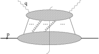
For fully inclusive DIS, the general structure of leading regions is symbolized in Fig. 2(b). The consequences for factorization are as follows. First, there may be extra collinear gluons exchanged between the proton-collinear subgraph and the hard-scattering subgraph. These gluons are allowed for [12, 13, 14, 15] when integrated pdf’s are defined with a Wilson line between the quark and antiquark fields; the resulting pdf’s are gauge invariant. A second complication is that hard scattering subprocess can be arbitrarily more complicated than the Born graph used in the handbag diagram. However, apart from the gluons that give the Wilson line factor, the hard scattering has the minimum possible number of external parton lines, to avoid losing a power of $Q$. A single graph can have many different regions, and this is correlated with the fact that the integrated pdf’s as defined below are UV divergent. However, the end result is that a valid factorization theorem holds if finite pdf’s are defined by ordinary UV renormalization of their UV divergences, and if the hard scattering coefficients are constructed with suitable subtractions. In that case we have a valid pdf defined by [13, 16]

$$f_{i}(x,\mu)=\int\frac{dy^{-}}{4\pi}\e^{-ixp^{+}y^{-}}\langle p|\,\bar{\psi}_{i}(0,y^{-},\bm{0}_{T})W[y,0]\gamma^{+}\psi_{i}(0)\,|p\rangle_{R}.$$ (7)

The lack of the ?? symbol indicates that this is a valid definition, as far as I know. Here $W[y,0]$ indicates a Wilson line (, a path-ordered exponential of the gluon field) along the light-like straight line from the point $0$ to $(0,y^{-},\bm{0}_{T})$. The subscript ‘$R$’ indicates that the operator is renormalized. The renormalization group equations for the dependence on the renormalization scale $\mu$ of pdf’s defined in this fashion are just the well-known DGLAP equations.

However, as we will see in Sec. 2.4.1, the presence of UV divergences removes the possibility of literally interpreting these pdf’s as number densities. The factorization formulae merely permit them to be used as if they are number densities, since the factorizations have the form of pdf’s convoluted with a short-distance cross section.

Another possible method of dealing with the UV divergences in the integral over all $\bm{k}_{T}$ is to define an integrated pdf by an integral over a restricted range $|\bm{k}_{T}|<Q$, as advocated by Brodsky and his collaborators [12, 17]:

$$f_{i}(x,Q)=\int_{|\bm{k}_{T}|<Q}d^{2}\bm{k}_{T}\,P_{i}(x,\bm{k}_{T}).~{}~{}\framebox{\small??}$$ (8)

As we will see in Sec. 2.4.1, the need for renormalizing the quark fields still gives difficulties with a number interpretation. More importantly, this definition has divergences — see Sec. 2.4.2 — associated with the use of the light-cone gauge (or of the corresponding light-like Wilson lines), contrary to the case when the integral is over all $\bm{k}_{T}$, as in Eq. (7). Observe that the DGLAP scale dependence with definition (8) arises not only from the explicit upper cutoff on $\bm{k}_{T}$ but also from the anomalous dimension of the quark fields in the definition of the unintegrated density $P_{i}(x,\bm{k}_{T})$.

2.4 Light-cone gauge

Fig. 2(b) has extra exchanged collinear gluons compared with the handbag diagram. One way of treating them [12] is to use light-cone gauge, $A^{+}=0$, where these gluons are power-suppressed. Correspondingly, the Wilson line $W[y,0]$ in Eq. (6) is unity in this gauge, so that one can try to define pdf’s by applying the non-gauge-invariant definitions (3), (4), and (6) in the $A^{+}=0$ gauge.

This is in fact the natural gauge for implementing light-front quantization, so that these definitions give an elegant interpretation of abstract operator definitions like Eq. (7), as expectation values of number operators.

Now, it is true that the divergences should cancel in a gauge-invariant physical quantity, like a cross section. So it could be argued that the divergences in theorists’ constructs like pdf’s are not really relevant. However the cancellation of divergences only holds if the physical quantity is computed exactly or in some particular given order of perturbation theory. Unfortunately, factorization provides approximations that mix different orders. For example, the result of a RG improved calculation of DIS structure function has the schematic form

$$F(Q)=f(\mu_{0})\exp\left[\int_{\mu_{0}}^{Q}\gamma(\alpha_{s}(\mu))\,d\mu/\mu\right]C(Q/\mu).$$ (9)

The value of the pdf $f(\mu_{0})$ is obtained from fits to data; it must be considered as exact, complete with all non-perturbative contributions. Both the evolution kernel $\gamma$ and the hard scattering coefficient $C$ are computed in perturbation theory truncated to some low order. The power of RG methods is that they show how make these approximations correctly and systematically.

The truncations of perturbation theory in the hard scattering factor and in the anomalous dimension in the exponent mean that an approximation to the structure function is not made at a single fixed order of perturbation theory. Therefore the use of factorization methods depends critically on all the factors being individually finite.

2.4.1 UV divergences

To maintain a strict number interpretation of the pdf’s, it is essential not only that the pdf’s defined by equations like Eq. (4) and (8) are finite, but also that the creation and annihilation operators have the standard commutation relations:

$$\left[{a_{i}}^{{\dagger}}(xp^{+},\bm{k}_{T},\lambda),{a_{j}}(x^{\prime}p^{+},\bm{k^{\prime}}_{T},\lambda^{\prime})\right]=\delta_{ij}\delta_{\lambda\lambda^{\prime}}(2\pi)^{3}2x\delta(x-x^{\prime})\delta^{(2)}(\bm{k}_{T}-\bm{k^{\prime}}_{T}).$$ (10)

These commutation relations follow, according to the principles of light-front quantization, from the canonical commutation relations for the bare field operators.

The important point is that it is the bare fields, not the renormalized fields that obey canonical commutation relations. On the other hand, finite matrix elements of fields are those with renormalized, not bare fields. Thus the ${a_{i}}^{{\dagger}}$ and ${a_{i}}$ operators in the definitions of the pdf’s must be those obtained from Fourier transforms of the renormalized fields. Since the bare and renormalized fields generally differ by an infinite factor, we must conclude that the pdf’s differ from actual number densities by infinite factors. These considerations are entirely separate from the issues recently discussed by Brodsky et al. under the title “Structure functions are not parton probabilities” [19].

As Brodsky et al. [17] explain, the UV problems can be evaded by choosing to work with a large UV cutoff. To avoid changing the physics, this cutoff must be much larger than all experimental energy scales. But the continuum limit cannot be taken.

From the point of view of factorization theorems, the issue of UV divergences is irrelevant. All that matters is that one has some well defined quantities that are labeled as pdf’s, and in terms of which useful factorization theorems are valid.

2.4.2 Light-cone gauge divergences

Harder issues arise because of some well-known problems with the light-cone gauge. These cause divergences beyond those associated with renormalization. Essentially identical problems arise if the pdf’s are defined gauge invariantly with light-like Wilson lines.

General results that show that these definitions give divergences in unintegrated pdf’s were obtained by Collins and Soper [16, 20]. They defined parton densities in an axial, or planar, gauge $n\cdot A=0$ with a non-light-like gauge fixing vector $n^{\mu}$. Then they derived an equation for the gauge dependence, and the solution of the equation gives a singular result in the light-cone-gauge limit. The result is valid at least to all orders of perturbation theory. Although the light-cone-gauge divergences cancel in the integrated pdf’s, they do not cancel in pdf’s integrated up to some finite limit. Thus the cutoff method of defining an integrated pdf, as in [17] Eq. (8), cannot be applied when the light-cone-gauge definition is used for the unintegrated pdf.

The technical derivation of the Collins-Soper equation was actually only given for unintegrated fragmentation functions. They and Sterman [9] stated the corresponding result for pdf’s, but did not give an actual proof. This equation has proved very useful in the analysis of transverse momentum distributions.

To verify the existence of a divergence, we now examine a one-loop calculation of the density of quarks in a quark. The results can readily be obtained with the aid of the Feynman rules in [16]. Perturbation-theory divergences associated with the masslessness of the gluon in QCD are irrelevant to our current purpose, as are the dimension of space-time and the non-abelian nature of the gauge group. So we will work with a gluon of nonzero mass $m_{g}$, which is consistent if the gauge group is abelian. We will also have a nonzero quark mass $m$. Thus we avoid actual IR and collinear divergences. We will use a space-time dimension $4-\epsilon$, so that the model is superrenormalizable; then no divergent wave-function renormalization of the fields is needed.

The lowest-order value is just a delta function: $P_{0}=\delta(1-x)\delta^{(2-\epsilon)}(\bm{k}_{T})$. The subscript “$0$” in “$P_{0}$” just indicates its order in perturbation theory, $\alpha_{s}^{0}$. The fact that the lowest order pdf is a delta function means that a numerical interpretation is given by integrating with an arbitrary smooth test function $t(x,\bm{k}_{T})$. Thus we write:

$$P_{0}[t]\equiv\int dx\,d^{2-\epsilon}\bm{k}_{T}\,t(x,\bm{k}_{T})\,P_{0}(x,\bm{k}_{T})=t(0,\bm{0}_{T}).$$ (11)

Treating the parton densities as generalized functions, to be “integrated with a test function” (to use the common abuse of mathematical terminology), will enable us to perform a proper analysis of the divergences in one-loop order and of their cancellation or lack of it.

The one-loop graphs for real gluon-emission graphs give

$$P_{1R}(x,\bm{k}_{T}) = \frac{g^{2}}{2(2\pi)^{3-\epsilon}}\left\{\frac{\displaystyle\frac{4}{1-x}-2-2x-\epsilon(1-x)}{k_{T}^{2}+m_{g}^{2}x+m^{2}(1-x)^{2}}\right.$$ (12)

$$\hskip 56.9055pt+\left.\frac{x(1-x)\left[-4m^{2}-2m_{g}^{2}+m_{g}^{2}\epsilon\right]}{\left[k_{T}^{2}+m_{g}^{2}x+m^{2}(1-x)^{2}\right]^{2}}\right\}.$$

The one-loop virtual graphs are proportional to a delta function. An explicit calculation shows that the coefficient is exactly the integral of the real emission graphs over all $x$ and $\bm{k}_{T}$, but with the sign changed:

$$P_{1V}(x,\bm{k}_{T})=-\delta(1-x)\,\delta^{(2-\epsilon)}(\bm{k}_{T})\int_{0}^{1}d\alpha\int d^{2-\epsilon}\bm{l}_{T}\,P_{1R}(\alpha,\bm{l}_{T}).$$ (13)

Observe that the $4/(1-x)$ term in the first line of Eq. (12) implies that $P_{1V}$ is divergent. If the calculation is done in light-cone gauge, the divergence is a direct consequence of the $1/k^{+}$ singularity in the gluon propagator. If the calculation is done in Feynman gauge, the divergence arises from the corresponding singularity in the Feynman rule for the Wilson line.

The divergence is caused by an endpoint singularity, so it cannot be removed by changing the analytic prescription for the singularity of the gluon propagator in light-cone gauge. See Brodsky et al. [17] for another calculation of the same divergence.

Given that divergences often cancel between real and virtual graphs, we should add the real and virtual contributions, which we must do in the sense of generalized functions, , with an integral with a test function:

$$\int dx\,d^{2-\epsilon}\bm{k}_{T}\,t(x,\bm{k}_{T})\,P_{1}(x,\bm{k}_{T})~{}=$$ (14)

$$=~{}\frac{g^{2}}{2(2\pi)^{3-\epsilon}}\int_{0}^{1}dx\int d^{2-\epsilon}\bm{k}_{T}\left[t(x,\bm{k}_{T})-t(1,\bm{0}_{T})\right]\times$$

$$\times\left\{\frac{\displaystyle\frac{4}{1-x}-2-2x-\epsilon(1-x)}{k_{T}^{2}+m_{g}^{2}x+m^{2}(1-x)^{2}}+\frac{x(1-x)\left[-4m^{2}-2m_{g}^{2}+m_{g}^{2}\epsilon\right]}{\left[k_{T}^{2}+m_{g}^{2}x+m^{2}(1-x)^{2}\right]^{2}}\right\}.$$

Since we are manipulating divergent integrals, we should actually apply a regulator (for example, we could apply a cut off on the plus momenta in the theory) in order to derive this formula correctly.

If the test function is replaced by a function independent of $\bm{k}_{T}$, then the divergence does cancel, because the factor $t(x,\bm{k}_{T})-t(1,\bm{0}_{T})$ becomes $t(x)-t(1)$, which is zero at $x=1$. This result was given by Collins and Soper [16]. Thus the integrated parton density does exist, in the sense of generalized functions.

However if the test function is $\bm{k}_{T}$ dependent, then the divergence does not generally cancel. In particular, if the integrated pdf were defined with an cutoff on transverse momentum, as in Eq. (8), it would have an uncanceled divergence.

2.4.3 Interpretation of light-cone gauge divergences

Examination of the derivation of the above results shows that the plus component of the gluon’s momentum is $(1-x)p^{+}$ [or $(1-\alpha)p^{+}$]. So at first sight the divergence at $x\to 1$ is a soft divergence, similar to the ones in QED. But since we have nonzero gluon and quark masses, this is not a correct interpretation; the divergence exists for any value of $\bm{k}_{T}$.

In fact the divergence comes from a region where the gluon rapidity goes to minus infinity. That is, it is from where the gluon is going infinitely fast in the direction of the outgoing quark jet (if we consider the corresponding DIS kinematics in the Breit frame, as in Fig. 1). It therefore corresponds to a region of momentum that has nothing to do with the region of momenta collinear to the proton that was associated with the pdf in deriving factorization. We must therefore say that we have an inappropriate definition of a pdf.

3 Correct definitions (I hope) of unintegrated pdf’s

The derivation of factorization involved making an approximation appropriate for certain regions of momenta, and the definition of the pdf arose from extrapolating this definition beyond the region of validity of the approximation.

3.1 Options

Since there are divergences in the pdf, as we have seen, the definition must be modified to incorporate some kind of cutoff on gluon rapidity or some kind of generalized renormalization. The cutoff must apply to gluons in virtual graphs. However, we should not implement the cutoff in the Lagrangian of QCD. For then the cutoff would depend on which hadron in a process we are considering, whereas the QCD Lagrangian is supposed to describe all possible processes on all possible momentum scales. Moreover we would simultaneously need opposite cutoffs for different parts of the same process. For example, we would need a cutoff on gluons of negative rapidity to define pdf’s in the target hadron in DIS, but we would a cutoff on gluons of positive rapidity to define the fragmentation function.

So the cutoff belongs in the definition of the operator whose expectation value is the parton density. There are several possibilities, including:

• Use the non-gauge-invariant definition Eq. (4), but choose the gauge to be an axial/planar gauge $n\cdot A=0$ with a non-light-like gauge fixing vector $n^{\mu}$, as proposed by Collins and Soper [16]. This is basically correct, but it does not contain the analytic properties associated with the directions of the Wilson lines that a correct Feynman-gauge derivation of factorization would naturally give. See [22, 11] for recent work on spin-dependent processes where the process-dependent direction of the Wilson line is critical to getting the correct relative signs for single spin asymmetries, which are non-universal between different processes.

• This problem can be overcome by inserting Wilson lines in non-light-like directions [23]. It is important that the derivation of a valid factorization produces certain constraints of the directions of the Wilson lines. It is not sufficient, for example, simply to choose the Wilson line to be along the straight lines joining the quark and antiquark field.

• Use the definition with light-like Wilson lines, but multiply by a suitable gauge-invariant factor that cancels the divergence. This was suggested by Collins and Hautmann [24] on the basis of a one-loop calculation. This gives a kind of generalized renormalization with the renormalization factors being certain vacuum expectation values of Wilson line operators, with a mixture of light-like and non-light-like lines. Their definition appears to follow almost uniquely from the structure of the asymptotics of one-loop graphs.

I propose that either of the last two methods is appropriate and valid, with the third method being the more elegant mathematically. Observe that simply using light-like Wilson lines without a further generalized renormalization factor does not remove the divergences.

All of these definitions involve two auxiliary parameters, a renormalization scale $\mu$ and an effective cutoff on gluon rapidity. Collins and Soper [16] introduced a parameter $\zeta$, which can be interpreted as $p^{2}\cosh^{2}\Delta y$, where $\Delta y$ is the difference of rapidity between the target hadron and the gluon rapidity cutoff.

These extra parameters mean that the pdf’s suitable for applying factorization depend on the energy of the process, thereby endangering universality of pdf’s. Universality, which allows the pdf’s to be used phenomenologically, is regained with the aid of evolution equations for the dependence on the auxiliary parameters. These were obtained by Collins, Soper, and Sterman [9, 16, 20]. Their equations are very different to the normal DGLAP equations, even though some of the physics content is related. Developments of these equations for understanding the large $x$ behavior of pdf’s have been obtained by Sterman [25].

3.2 Non-light-like Wilson line

The first option is to define the unintegrated pdf’s gauge-invariantly with non-light-like Wilson lines. Just as in Eq. (6), the pdf is a Fourier transform:

$$P_{i}(x,\bm{k}_{T},\zeta,\mu)=\int\frac{dy^{-}\,d^{2}\bm{y}_{T}}{16\pi^{3}}\e^{-ixp^{+}y^{-}+i\bm{k}_{T}\cdot\bm{y}_{T}}\,\tilde{P}_{i}(y^{-},\bm{y}_{T},\zeta,\mu),$$ (15)

but where the quark correlation function has Wilson line factors:

$$\tilde{P}_{i}(y^{-},\bm{y}_{T},\zeta,\mu)=\langle p|\,\bar{\psi}_{i}(0,y^{-},\bm{y}_{T})\,W_{y}(u)^{{\dagger}}\,I_{u;y,0}\,\gamma^{+}\,W_{0}(u)\,\psi_{i}(0)\,|p\rangle_{R}.$$ (16)

Here $W_{y}(u)$ denotes the following Wilson line operator

$$W_{y}(u)=P\exp\left[-ig_{(0)}\int_{0}^{\infty}d\lambda\,u^{\mu}\,A_{\mu}^{(0)}(y+\lambda u)\right],$$ (17)

where the line is from the position $y^{\mu}$ going to infinity in the direction $u^{\mu}$. To make the definition exactly gauge-invariant, a Wilson line $I_{u;y,0}$ at infinity is needed [26] to join $W_{y}(u)$ and $W_{0}(u)$. In Feynman gauge this line at infinity can be replaced by unity. Note the following

• This gives a gauge invariant definition of the unintegrated pdf, with the coupling and the gauge field being the bare quantities, as indicated by the sub/superscript “$(0)$”.

• The vector $u^{\mu}$ that sets the direction of the Wilson line must not be light-like. The parton density therefore depends on the variable $\zeta=(p\cdot u)^{2}/u^{2}$.

• According to [9, 20], the proof of a factorization theorem requires that $u^{\mu}$ should be approximately “at rest” in the center of mass of the hard scattering. Thus the Wilson lines are used, roughly speaking, to separate the gluons associated with different jets.

• Hence $\zeta\sim s$, the square of the center-of-mass energy. Refs. [9, 20] give an equation for the $\zeta$ dependence of the pdf.

• Strict gauge invariance requires that the two Wilson lines be connected by a link at infinity, $I_{u;y,0}$, as Belitsky, Ji, and Yuan [26] have observed. When Feynman gauge is used, at least in simple calculations, this extra link does not contribute. But in light-cone gauge, the link at infinity is the only part of the Wilson line that contributes, and is critical in obtaining correct values for time-reversal-odd pdf’s.

• Whether $u^{\mu}$ points to the future or past depends on the process. For DIS-type process a future pointing line is needed, which corresponds to final-state interactions in the Breit frame. For DY-type processes a past-pointing line, associated with initial-state interactions in the center-of-mass, is needed. Time reversal invariance can be used to relate the two cases [11], and gives a reversal of sign for time-reversal-odd pdf’s.

• There are UV divergences associated with the quark-Wilson-line vertex that must be renormalized away by conventional methods. This is indicated by the subscript “$R$” in Eq. (16).

3.3 Light-like Wilson line with generalized renormalization

The definition Eq. (16) is a gauge-invariant transcription and correction of the planar-gauge definition by Collins and Soper [16]. However, the non-light-like Wilson lines complicate explicit Feynman graph calculations, compared with those that use light-like Wilson lines. There is also a mathematical problem. The exact evolution equation has an inhomogeneous term that is power-suppressed and that is ignored in applications. It would be preferable to have an exactly homogeneous equation.

Figure 3: Diagrammatic interpretation of Eq. (18). This is ordinary pdf in coordinate space (with a light-like Wilson line) divided by the vacuum expectation value of a certain pure Wilson line operator. Any number of gluon lines can join the lower blob to the top Wilson line in the numerator. Any number of gluon lines can join the Wilson lines in the denominator.

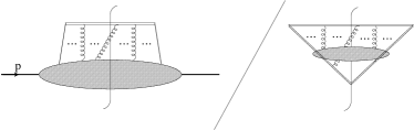
I therefore propose an alternative definition. A light-like Wilson line is used in Eq. (16) and the consequent divergences are canceled by a kind of generalized renormalization factor. From the work of Collins and Hautmann [24], I conjecture that a valid definition is

$$\tilde{P}^{\rm alt}_{i}(y^{-},\bm{y}_{T},\zeta,\mu)=\frac{\langle p|\,\bar{\psi}_{i}(0,y^{-},\bm{y}_{T})\,W_{y}(n)^{{\dagger}}\,I_{n;y,0}\,\gamma^{+}\,W_{0}(n)\,\psi_{i}(0)\,|p\rangle_{R}}{\langle 0|\,W_{y}(n)^{{\dagger}}\,W_{y}(u^{\prime})\,I_{n;y,0}\,I_{u^{\prime};y,0}^{{\dagger}}\,W_{0}(n)\,W_{0}(u^{\prime})^{{\dagger}}\,|0\rangle_{R}}.$$ (18)

This is illustrated in Fig. 3. The Wilson line associated with the quark fields is now in an exactly light-like direction $n^{\mu}=(n^{+},n^{-},\bm{n}_{T})=(0,\pm 1,\bm{0}_{T})$, which is future pointing or past pointing depending on the process [11]. The vector ${u^{\prime}}^{\mu}$ in the Wilson line in the denominator plays the role of the vector $u^{\mu}$ in the previous definition. The pdf is defined by taking $n^{\mu}$ initially non-light-like, computing the ratio in Eq. (18), and then taking the limit that $n^{\mu}$ is light-like. One-loop calculations [24, 27] indicate that this can be implemented by a subtraction method.

4 Summary

4.1 Integrated pdf’s

• Integrated pdf’s can be defined by formulae like Eq. (7). They involve an integral over all transverse momentum, strictly out to infinity. The resulting UV divergences are removed by conventional renormalization.

• Factorization theorems containing these pdf’s have been proved for various inclusive processes [14, 15, 28].

• In this formalism, the DGLAP equations are exactly the renormalization-group equations for the pdf’s

• Divergences associated with the use of light-cone gauge or of light-like Wilson lines cancel after the integral to infinite transverse momentum

• The presence of UV divergences prevents a literal number interpretation of these pdf’s. Even so, momentum and quark-number sum rules are exact, provided a suitable renormalization scheme is used, , $\overline{\rm MS}$. The proof [16] relates the relevant moments of the pdf’s to matrix elements of conserved Noether currents.

4.2 Unintegrated pdf’s

• The most obvious definitions of unintegrated pdf’s, , of transverse-momentum-dependent pdf’s, are plagued with divergences associated with the use of light-cone gauge, or with the corresponding light-like Wilson lines.

• Some kind of cut-off or generalized renormalization must be apply to remove these divergences.

• Two possible definitions are proposed, in Eqs. (15), (16), and (18).

• One of these is a gauge invariant transcription of the Collins-Soper definition [16]; the other is a potential improvement better adapted to subtractive methods of proof and calculation.

• Given the auxiliary steps needed to define the unintegrated pdf’s, it does not appear that they have a literal number interpretation. One uses them in factorization theorems as if they are number densities, but the strict number interpretation is not needed.

• Given the extra cutoff needed on gluon rapidity, one should not expect that the integral over transverse momentum of an unintegrated pdf should be exactly the corresponding integrated pdf. The relation between the two involves a non-trivial but perturbatively calculable coefficient [16, 20].

• The existence of the extra cutoff implies that phenomenological applications should use an evolution equation [16, 20, 9] for the dependence of the unintegrated pdf on this cutoff.

4.3 What needs to be done

The reader who tries to find detailed justification for many of the statements in this article will probably be quite frustrated. If nothing else, the literature on the subject is very fragmented. Many results which are reasonably clear to experts in the field, , as minor modifications to previously existing results, are quite unobvious to outsiders and newcomers.

Moreover, published definitions of pdf’s taken literally often give divergences. Given the great importance of pdf’s and factorization theorems to the whole of high-energy physics, it is important to fully systematize the subject.

In this paper I have attempted to make a contribution to this systematization by presenting what I believe to be complete definitions of pdf’s for quarks, with all known sources of divergences explained and explicitly overcome by suitable prescriptions for (generalized) renormalization and/or cutoff. These should, of course, be useful for the precise formulation of higher-order perturbative QCD calculations. But they should also be for providing a fully and rigorously defined interface to models of non-perturbative hadronic structure that are becoming increasingly important.

It is with pleasure that I dedicate this work to Jan Kwieciński.

References

- [1] R.K. Ellis, W.J. Stirling and B.R. Webber, QCD and collider physics (Cambridge University Press, 1996).
- [2] J.C. Collins, D.E. Soper and G. Sterman, Factorization Of Hard Processes In QCD, in Perturbative QCD (A.H. Mueller, ed.) (World Scientific, Singapore, 1989).
- [3] R. Brock et al. [CTEQ Collaboration], Rev. Mod. Phys. 67, 157 (1995);
- [4] R.P. Feynman, Photon–Hadron Interactions (Benjamin, 1972).
- [5] C. Bouchiat, P. Fayet and P. Meyer, Nucl. Phys. B 34, 157 (1971).
- [6] D.E. Soper, Phys. Rev. D 15, 1141 (1977).
- [7] D.E. Soper, Phys. Rev. Lett. 43, 1847 (1979).
- [8] J.W. Negele and H. Orland, Quantum Many-Particle Systems (Addison Wesley, 1988).
- [9] J.C. Collins, D.E. Soper and G. Sterman, Nucl. Phys. B 250, 199 (1985).
-
[10]
D.W. Sivers,
Phys. Rev. D 41, 83 (1990)
[Annals Phys. 198, 371 (1990)].
D.W. Sivers, Phys. Rev. D 43, 261. (1991)
M. Anselmino, M. Boglione and F. Murgia, Phys. Lett. B 362, 164 (1995) [arXiv:hep-ph/9503290].
P.J. Mulders and R.D. Tangerman, Nucl. Phys. B 461, 197 (1996) [Erratum-ibid. 484, 538 (1997)] [arXiv:hep-ph/9510301].
D. Boer and P.J. Mulders, Phys. Rev. D 57, 5780 (1998) [arXiv:hep-ph/9711485].
M. Anselmino and F. Murgia, Phys. Lett. B 442, 470 (1998) [arXiv:hep-ph/9808426].
D. Boer, Phys. Rev. D 60, 014012 (1999) [arXiv:hep-ph/9902255].
L.P. Gamberg, G.R. Goldstein and K.A. Oganessyan, arXiv:hep-ph/0301018. - [11] J.C. Collins, Phys. Lett. B 536, 43 (2002), [arXiv:hep-ph/0204004].
- [12] G.P. Lepage and S.J. Brodsky, Phys. Rev. D 22, 2157 (1980).
- [13] A.V. Efremov and A.V. Radyushkin, Theor. Math. Phys. 44, 774 (1981) [Teor. Mat. Fiz. 44, 327 (1980)].
- [14] J.C. Collins, D.E. Soper and G. Sterman, Nucl. Phys. B 261, 104 (1985).
- [15] J.C. Collins, D.E. Soper and G. Sterman, Nucl. Phys. B 308, 833 (1988).
- [16] J.C. Collins and D.E. Soper, Nucl. Phys. B 194, 445 (1982).
- [17] S.J. Brodsky, D.S. Hwang, B.Q. Ma and I. Schmidt, Nucl. Phys. B 593, 311 (2001) [arXiv:hep-th/0003082].
- [18] R.L. Jaffe, Nucl. Phys. B 229, 205 (1983).
- [19] S.J. Brodsky, P. Hoyer, N. Marchal, S. Peigné and F. Sannino, Phys. Rev. D 65, 114025 (2002) [arXiv:hep-ph/0104291].
- [20] J.C. Collins and D.E. Soper, Nucl. Phys. B 193, 381 (1981). [Erratum—ibid. 213, 545 (1981)].
- [21] F. Landry, R. Brock, P.M. Nadolsky and C.P. Yuan, arXiv:hep-ph/0212159.
- [22] S.J. Brodsky, D.S. Hwang and I. Schmidt, Phys. Lett. B 530, (2002) 99 [arXiv:hep-ph/0201296].
- [23] J.C. Collins, Sudakov form factors, in Perturbative QCD (A.H. Mueller, ed.) (World Scientific, Singapore, 1989).
[24]
J.C. Collins and F. Hautmann,
Phys. Lett. B 472, 129 (2000),
[arXiv:hep-ph/9908467].
J.C. Collins and F. Hautmann, JHEP 03, 016 (2001), [arXiv:hep-ph/0009286]. - [25] G. Sterman, Nucl. Phys. B 281, 310 (1987).
[26]
A.V. Belitsky, X. Ji and F. Yuan,
Nucl. Phys. B 656, 165 (2003)
[arXiv:hep-ph/0208038].
X. Ji and F. Yuan, Phys. Lett. B 543, 66 (2002) [arXiv:hep-ph/0206057]. - [27] J.C. Collins and A. Metz, in preparation.
- [28] G.T. Bodwin, Phys. Rev. D 31, 2616 (1985) [Erratum — ibid. 34, 3932 (1986)].