Direct $J/\psi$ and $\psi^{\prime}$ hadroproduction via fragmentation in collinear parton model and $k_{T}$-factorization approach

Abstract

The $p_{T}$-spectra for direct $J/\psi$ and $\psi^{\prime}$ in hadroproduction at Tevatron energy have been calculated within the framework of the NRQCD formalism and the fragmentation model in the collinear parton model as well as in the $k_{T}$-factorization approach. We have described the CDF data and obtained a good agreement between the predictions of the parton model and the $k_{T}$-factorization approach. We performed the calculations using the relevant leading order in $\alpha_{s}$ hard amplitudes and taking equal values of the long-distance matrix elements for the both models.

I Introduction

During the years after the measuring of charmonium productiom cross sections and polarization effects for $J/\psi$ and $\psi^{\prime}$ mesons at the Tevatron Collider 1 the phenomenology of a quarkonium production has a phase of intensive developments. Nowadays, it is understand that the heavy quarkonium production is a very complicated physical process needs many new theoretical ideas. Starting from the Color Singlet Model 2 it was developed, so-called, the nonrelativistic QCD (NRQCD) formalism 3 to describe the nonperturbative transition of $Q\bar{Q}$-pair into a final heavy quarkonium.

The perturbative fragmentation functions for partons which split into heavy quarkonia have been obtained 4 within the framework of the NRQCD formalism. It is supposed that the fragmentation model is more adequate for the description of a quarkonium production at the large quarkonium transverse momentum $p_{T}\gg M_{Q\bar{Q}}$ than the fusion model.

In the charmonium production at the energy range of the Tevatron Collider we deal with the gluon distribution function from a proton which is taken at a very small $x$ but the relevant virtuality $\mu^{2}\sim M_{Q\bar{Q}}^{2}+p_{T}^{2}$ is large. In the region under consideration the collinear parton model can be generalized within the framework of the $k_{T}-$factorization approach 5a ; 5b ; 5c ; 5d . This fact leads to some interesting effects in the quarkonium production at the high energies, which were discussed ten years ago in Ref. 6 and recently in Refs. 7 ; 7a ; 7b ; 7c .

In this paper we calculate the $p_{T}$-spectra of the unpolarized direct $J/\psi$ and $\psi^{\prime}$ mesons produced via the fragmentation mechanism. In case of direct $J/\psi$ and $\psi^{\prime}$ it is supposed that the production via the gluon fragmentation into the color-octet $Q\bar{Q}$ [${}^{3}S_{1},\underline{8}$] state is a dominant contribution 8 ; 9 . We compare the predictions which are obtained as in the collinear parton model as in the $k_{T}$-factorization approach. In both cases we performed calculations with the hard amplitudes in the leading order of the QCD running constant $\alpha_{s}$. So, in the collinear parton model we take into consideration the partonic subprocess:

$$g+g\to g+g.$$ (1)

In the $k_{T}$-factorization approach we take into consideration the subprocess with off-shell or reggeized initial gluons:

$$g^{*}+g^{*}\to g.$$ (2)

We have described the CDF data 1 and obtained a good agreement between the parton model and the $k_{T}$-factorization calculations based on the hard amlitudes for subprocesses (1) and (2) with the equal values of the long-distance matrix elements $<{\cal O}^{J/\psi}[^{3}S_{1},8]>$ and $<{\cal O}^{\psi^{\prime}}[^{3}S_{1},8]>$ in the fragmentation functions $D_{g\to J/\psi,\psi^{\prime}}(z,\mu^{2})$ for the both models. The QCD evolution of the fragmentation function is described by the homogeneous equation with a boundary condition proportional to the delta function $\delta(1-z)$.

The results obtained in the paper within the $k_{T}$-factorization approach based on the fragmentation function model differ from results of Refs. 7a ; 7b ; 7c , which were obtained using the gluon fusion model. The possible reasons of a disagreement will be discuss below.

II NRQCD formalism

Within the framework of the NRQCD, the cross section or the fragmentation function for a quarkonium $H$ production can be expressed as a sum of terms, which are factorized into a short-distance coefficient and a long-distance matrix element 3 :

$$d\sigma(H) = \sum_{n}d\hat{\sigma}(Q\bar{Q}[n])<{\cal O}^{H}[n]>,$$ (3)

$$D(a\to H) = \sum_{n}D(a\to Q\bar{Q}[n])<{\cal O}^{H}[n]>.$$ (4)

Here the $n$ denotes the set of color and angular momentum numbers of the $Q\bar{Q}$ pair, which production cross section is $d\hat{\sigma}(Q\bar{Q}[n])$ or which fragmentation function is $D(a\to Q\bar{Q}[n])$. Last ones can be calculated perturbatively in the strong coupling $\alpha_{s}$. Of course, in the case of production in a hadron collision, the short-distance cross-section $d\hat{\sigma}$ have to be convoluted with the parton distribution function from the hadrons. The nonperturbative transition from the $Q\bar{Q}$ state $n$ into the final quarkonium $H$ is described by a long-distance matrix element $<{\cal O}^{H}[n]>$ which have to be calculated using non perturbative methods or determined from experimental data. The fit of the Tevatron data for the $p_{T}$-spectra of $J/\psi$, $\psi^{\prime}$ and $\chi_{c}$ charmonium states have been done recently by different authors (see review in Ref. 10 ). As it was shown in Refs. 8 ; 9 , at the large charmonium transverse momentum ($p_{T}>7$ GeV) the gluon fragmentation into color-octet state

$$g^{*}\to Q\bar{Q}[^{3}S_{1},8]$$ (5)

gives dominated contribution to the direct $J/\psi$ and $\psi^{\prime}$ hadroproduction. The values of the color-octet matrix elements under consideration are following $<{\cal O}^{J/\psi}[^{3}S_{1},8]>$=$4.4\cdot 10^{-3}$ GeV³, $<{\cal O}^{\psi^{\prime}}[^{3}S_{1},8]>$=$4.2\cdot 10^{-3}$ GeV³ 9 . Note, that the fit of CDF data for the $p_{T}$-spectrum of a direct $J/\psi$ production within the framework of the fusion model in the collinear parton model gives the another numerical value of the long-distance matrix element $<{\cal O}^{J/\psi}[^{3}S_{1},8]>$=$1.2\cdot 10^{-2}$ GeV³ 10 . It will be important to compare the results obtained in the $k_{T}$-factorization approach based on the fusion and fragmentation models.

III Fragmentation function

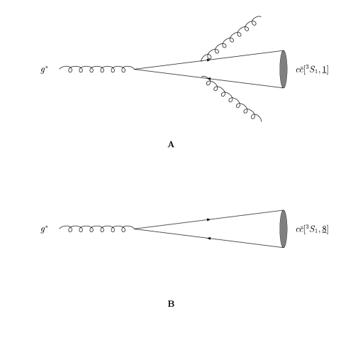
Figure 1: Diagrams used for description LO in the $\alpha_{s}$ fragmentation $g^{*}\to J/\psi gg$ (color-singlet state, A) and $g^{*}\to J/\psi$ (color-octet state, B).

The gluon fragmentation into ${}^{3}S_{1}$ charmonium state is determined by the color-singlet (Fig.1,a) and the color-octet (Fig.1,b) contributions. The previous analysis has shown that the probability of a gluon fragmentation into the color-singlet state is only a small part of the probability of a fragmentation into the color-octet state 8 . The leading order in the $\alpha_{s}$ fragmentation functions for the transition (4) are known and can be written at the scale $\mu^{2}=\mu^{2}_{0}=4m_{c}^{2}$ as follows 4 :

$$D^{T}_{g\to J/\psi,\psi^{\prime}}(z,\mu^{2})=2d^{T}(z,\mu_{0}^{2})<{\cal O}^{J/\psi,\psi^{\prime}}[^{3}S_{1},8]>,$$ (6)

$$D^{L}_{g\to J/\psi,\psi^{\prime}}(z,\mu^{2})=d^{L}(z,\mu_{0}^{2})<{\cal O}^{J/\psi,\psi^{\prime}}[^{3}S_{1},8]>,$$ (7)

where

$$d^{T}(z,\mu_{0}^{2})=\frac{\pi\alpha_{s}(\mu_{0}^{2})}{48m_{c}^{3}}\delta(1-z)$$ (8)

$$d^{L}(z,\mu_{0}^{2})=\frac{\alpha_{s}^{2}(\mu_{0}^{2})}{8m_{c}^{3}}\frac{(1-z)}{z}.$$ (9)

It is obviously that the probability of the gluon fragmentation into the longitudinally polarized charmonium is negligibly small and $J/\psi$ or $\psi^{\prime}$ mesons have transverse polarization.

The fragmentation functions (7) and (8) are evolved in $\mu^{2}$ using the standard homogeneous DGLAP evolution equation 11 :

$$\mu^{2}\frac{\partial D_{g}}{\partial\mu^{2}}(z,\mu^{2})=\frac{\alpha_{s}(\mu^{2})}{2\pi}\int_{z}^{1}\frac{dx}{x}P_{gg}(\frac{x}{z})D_{g}(x,\mu^{2}),$$ (10)

where $P_{gg}(x)$ is the usual leading order gluon-gluon splitting function. To solve equation (9) we use the well known method based on Mellin transform. It is easy to obtain that the Mellin-momentum at the scale $\mu^{2}$ can be written as follows

$$D_{g}(n,\mu^{2})=D_{g}(n,\mu_{0}^{2})\exp\Biggl{[}\frac{P_{gg}(n)}{2\pi}\int_{\mu_{0}^{2}}^{\mu^{2}}\frac{d\mu^{2}}{\mu^{2}}\alpha_{s}(\mu^{2})\Biggr{]},$$ (11)

where

$$P_{gg}(n)=3\biggl{[}-2S_{1}(n)+\frac{11}{6}+\frac{2}{n(n-1)}+\frac{2}{(n+1)(n+2)}\biggr{]}-1,$$ (12)

$$S_{1}(n)=\sum_{j=1}^{n}\frac{1}{j}.$$

In the one-loop approximation for the running constant $\alpha_{s}(\mu^{2})$ with the three active flavors ($b_{0}=9$) one has

$$\alpha_{s}(\mu^{2})=\frac{4\pi}{b_{0}\log(\mu^{2}/\Lambda^{2})},$$ (13)

and equation (10) can be presented as follows

$$D_{g}(n,\mu^{2})=D_{g}(n,\mu_{0}^{2})\exp\Biggl{[}\frac{2}{b_{0}}P_{gg}(n)\log\biggl{(}\frac{\log(\mu^{2}/\Lambda^{2})}{\log(\mu_{0}^{2}/\Lambda^{2})}\biggr{)}\Biggr{]}.$$ (14)

Taking into consideration that

$$D_{g}^{T}(n,\mu_{0}^{2})=\frac{\pi\alpha_{s}(\mu_{0}^{2})}{24m_{c}^{3}}<{\cal O}^{J/\psi,\psi^{\prime}}[^{3}S_{1},8]>$$ (15)

we have performed inverse Mellin transform numerically using following rule

$$D_{g}(z,\mu^{2})\approx D_{g}^{T}(z,\mu^{2})=\int_{C}dnz^{-n}D_{g}^{T}(n,\mu^{2}).$$ (16)

The integration contour $C$ can be transformed such as

$$D_{g}(z,\mu^{2})=\frac{1}{\pi}\int_{0}^{\infty}dt\quad\mbox{Im}\left[e^{i\phi}z^{-n}D_{g}^{T}(n,\mu^{2})\right],$$ (17)

where $n=c+te^{i\phi}$ and $c\approx 2$, $\phi=\displaystyle{\frac{\pi}{2}}$. In Fig.2 the obtained fragmentation function $D_{g\to J/\psi}(z,\mu^{2})$ multiplied by $10^{4}$ is shown at the different $\mu^{2}=30,100$ and $300$ GeV². We see that our result at the $\mu^{2}=300$ GeV² agrees well with the same one obtained in Ref. 12 . In a stage of convoluting of the fragmentation function $D_{g\to J/\psi}(z,\mu^{2})$ with the partonic cross section for the subprocesses (1) or (2) we will use the following definition for the variable $z$:

$$z=\frac{E_{\psi}+|\vec{p}_{\psi}|}{2E_{g}}$$ (18)

Thus we consider that the massless parton fragments into the massive meson. As it will be seen the definition (18) is more correct at a not so large $p_{T}$ than the massless one between the parton 4-momentum and the meson 4-momentum

$$p_{\psi}^{\mu}=zp_{g}^{\mu}.$$ (19)

We suggest also that meson has a small transverse momentum respectively initial gluon jet and we approximately can accept that in the laboratory frame

$$\eta_{\psi}\cong\eta_{g},$$ (20)

where $\eta_{\psi},\eta_{g}$ are the meson and gluon pseudorapidities.

Within the framework of the fragmentation model, the meson production cross section and the relevant gluon production cross section are connected as follows

$$\hat{\sigma}(gg\to J/\psi X)=\int dzD_{g\to J/\psi}(z,\mu^{2})\hat{\sigma}(gg\to gg)$$ (21)

or

$$\hat{\sigma}(g^{*}g^{*}\to J/\psi X)=\int dzD_{g\to J/\psi}(z,\mu^{2})\hat{\sigma}(g^{*}g^{*}\to g).$$ (22)

IV Leading order hard amplitudes

The squared amplitude for the partonic process (1) is well known and it can be presented as follows

$$\overline{|M(gg\to gg)|^{2}}=18\pi^{2}\alpha_{s}^{2}\frac{(\hat{s}^{4}+\hat{t}^{4}+\hat{u}^{4})(\hat{s}^{2}+\hat{t}^{2}+\hat{u}^{2})}{(\hat{s}\hat{t}\hat{u})^{2}},$$ (23)

where $\hat{s}$, $\hat{t}$ and $\hat{u}$ are usual Mendelstam variables.

There two approaches for calculation of a partonic amplitude for the subprocess (2) in the $k_{T}$-factorization approach 5b ; 5d . The effective Feynman rules for processes with off-shell gluons were suggested in Ref. 5b . The special trick is a choice of the initial gluon polarization 4-vector as follows

$$\varepsilon^{\mu}(k_{T})=\frac{k_{T}^{\mu}}{|\vec{k}_{T}|}.$$ (24)

In Ref. 5d the initial gluons are considered as reggeons (reggeized gluons) and the effective Reggeon-Reggeon-Gluon vertex function was obtained

$$C^{\lambda}(k_{1},k_{2})=-(k_{1}-k_{2})^{\lambda}+P_{1}^{\lambda}\left(\frac{k_{1}^{2}}{(kP_{1})}+2\frac{(kP_{2})}{(P_{1}P_{2})}\right)-P_{2}^{\lambda}\left(\frac{k_{2}^{2}}{(kP_{2})}+2\frac{(kP_{1})}{(P_{1}P_{2})}\right),$$ (25)

where $P_{1}=\frac{\sqrt{s}}{2}(1,0,0,1)$ and $P_{1}=\frac{\sqrt{s}}{2}(1,0,0,-1)$ are the colliding protons 4-momenta, $k_{1}=x_{1}P_{1}+k_{1T}$ and $k_{2}=x_{2}P_{2}+k_{2T}$ are the initial gluons 4-momenta, $k_{T}=(0,\vec{k}_{T},0)$, $k=k_{1}+k_{2}$ is the final real gluon 4-momentum. It is easy to show that vertex function $C^{\lambda}(k_{1},k_{2})$ satisfies the gauge invariance condition $(k_{1}+k_{2})_{\lambda}C^{\lambda}(k_{1},k_{2})=0$.

Omitting the color factor $f^{abc}$ we can write the amplitude of the subprocess (2) accordingly Ref.5b as follows

$${\cal M}=-g\varepsilon^{\lambda}(k)\frac{k_{1T}^{\mu}k_{2T}^{\nu}}{|\vec{k}_{1T}||\vec{k}_{2T}|}\left[(k+k_{1})_{\nu}g_{\lambda\mu}+(-k_{1}+k_{2})_{\lambda}g_{\mu\nu}+(-k_{1}-k)_{\mu}g_{\nu\lambda}\right].$$ (26)

We have obtained after simple transformations that

$${\cal M}=-\frac{g\varepsilon^{\lambda}(k)}{2|\vec{k}_{1T}||\vec{k}_{2T}|}x_{1}x_{2}s\tilde{C_{\lambda}}(k_{1},k_{2}),$$ (27)

where

$$\tilde{C^{\lambda}}(k_{1},k_{2})=-(k_{1}-k_{2})^{\lambda}+\frac{2P_{1}^{\lambda}}{x_{2}s}\left(k_{1}^{2}+x_{1}x_{2}s\right)-\frac{2P_{2}^{\lambda}}{x_{1}s}\left(k_{2}^{2}+x_{1}x_{2}s\right)=C^{\lambda}(k_{1},k_{2}).$$ (28)

Such a way, the approaches 5b ; 5d are equivalent and give the equal answer for the squared vertex function and amplitude:

$$C^{\lambda}(k_{1},k_{2})C_{\lambda}(k_{1},k_{2})=-\frac{4k_{1}^{2}k_{2}^{2}}{x_{1}x_{2}s},$$ (29)

and

$$\overline{|M(g^{*}g^{*}\to g)|^{2}}=\frac{3}{2}\pi\alpha_{s}\vec{p}_{T}^{2},$$ (30)

where $\vec{p}_{T}^{2}=(\vec{k}_{1T}+\vec{k}_{2T})^{2}=x_{1}x_{2}s$, $\vec{p}_{T}$ is the transverse momentum of the final gluon.

V Cross sections for the process $pp\to J/\psi(\psi^{\prime})X$

In the conventional collinear parton model it is suggested that hadronic cross section, in our case, $\sigma(pp\to J/\psi X,s)$, and the relevant partonic cross section $\hat{\sigma}(gg\to J/\psi X,\hat{s})$ are connected as follows

$$\sigma^{PM}(pp\to J/\psi,s)=\int dx_{1}\int dx_{2}G(x_{1},\mu^{2})G(x_{2},\mu^{2})\hat{\sigma}(gg\to J/\psi,\hat{s}),$$ (31)

where $\hat{s}=x_{1}x_{2}s$, $G(x,\mu^{2})$ is the collinear gluon distribution function in a proton, $x_{1,2}$ are the fraction of a proton momentum, $\mu^{2}$ is the typical scale of a hard process. The $\mu^{2}$ evolution of the gluon distribution $G(x,\mu^{2})$ is described by DGLAP evolution equation 11 .

In the $k_{T}$-factorization approach hadronic and partonic cross sections are related by the following condition 5a ; 5b ; 5c :

$$\sigma^{KT}(pp\to J/\psi X)=\int\frac{dx_{1}}{x_{1}}\int d{\vec{k}_{1T}^{2}}\int\frac{d\phi_{1}}{2\pi}\Phi(x_{1},\vec{k}_{1T}^{2},\mu^{2})$$ (32)

$$\int\frac{dx_{2}}{x_{2}}\int d{\vec{k}_{2T}^{2}}\int\frac{d\phi_{2}}{2\pi}\Phi(x_{2},\vec{k}_{2T}^{2},\mu^{2})\hat{\sigma}(g^{*}g^{*}\to J/\psi X,\hat{s}),$$

where $\hat{\sigma}(g^{*}g^{*}\to J/\psi X,\hat{s})$ is the $J/\psi$ production cross section on off-shell gluons, $k_{1}^{2}=k_{1T}^{2}=-\vec{k}_{1T}^{2}$, $k_{2}^{2}=k_{2T}^{2}=-\vec{k}_{2T}^{2}$, $\hat{s}=x_{1}x_{2}s-(\vec{k}_{1T}+\vec{k}_{2T})^{2}$, $\phi_{1,2}$ are the azimuthal angles in the transverse $XOY$ plane between vectors $\vec{k}_{1T}(\vec{k}_{2T})$ and the fixed $OX$ axis ($\vec{p}_{\psi}\in XOZ$). The unintegrated gluon distribution function $\Phi(x_{1},\vec{k}_{1T}^{2},\mu^{2})$ satisfies the BFKL evolution equation 13 .

Our calculation in the parton model is down using the GRV LO 14 and CTEQ5L 15 parameterizations for a collinear gluon distribution function $G(x,\mu^{2})$. In case of the $k_{T}$-factorization approach we use the following parameterizations for an unintegrated gluon distribution function $\Phi(x_{1},\vec{k}_{1T}^{2},\mu^{2})$: JB by Bluemlein 16 , JS by Jung and Salam 17 , KMR by Kimber, Martin and Ryskin 18 . The direct comparison between different parameterizations as functions of $x$, $\vec{k}_{T}^{2}$ and $\mu^{2}$ was presented in paper 7 .

The doubly differential cross sections for the process $pp\to J/\psi(\psi^{\prime})X$ can written as follows

$$\frac{d\sigma^{PM}}{d\eta_{\psi}dp_{\psi T}}=\int dx_{1}\int dzG(x_{1},\mu^{2})G(x_{2},\mu^{2})D_{g\to\psi}(z,\mu^{2})\frac{p_{gT}E_{g}}{E_{\psi}}\frac{\overline{|M(gg\to gg)|^{2}}}{8\pi x_{1}x_{2}s(u+x_{1}s)},$$ (33)

where

$$u=-\sqrt{s}(E_{g}-p_{gz}),\quad t=-\sqrt{s}(E_{g}+p_{gz}),\quad x_{2}=-\frac{x_{1}t}{u+x_{1}s},\quad x_{1,min}=-\frac{u}{s+t},$$

$$\hat{t}=x_{1}t,\quad\hat{u}=x_{2}u,\quad\hat{s}=x_{1}x_{2}s;$$

$$\frac{d\sigma^{KT}}{d\eta_{\psi}dp_{\psi T}}=\int dz\int d\phi_{1}\int d\vec{k}_{1T}^{2}\Phi(x_{1},\vec{k}_{1T}^{2},\mu^{2})\Phi(x_{2},\vec{k}_{2T}^{2},\mu^{2})D_{g\to\psi}(z,\mu^{2})\frac{E_{g}}{p_{gT}E_{\psi}}\frac{\overline{|M(g^{*}g^{*}\to g)|^{2}}}{x_{1}x_{2}s},$$ (34)

where

$$\vec{k}_{2T}=\vec{p}_{gT}-\vec{k}_{1T},\quad x_{1}=\frac{E_{g}+p_{gz}}{\sqrt{s}},\quad x_{2}=\frac{E_{g}-p_{gz}}{\sqrt{s}}.$$

The energy $(E_{g})$ of a fragmenting gluon and the energy of a final meson $(E_{\psi})$ are related as follows

$$E_{g}=\frac{E_{\psi}+|\vec{p}_{\psi}|}{2z},\quad|\vec{p}_{\psi}|=\frac{p_{\psi T}}{\sin(\theta_{\psi})},\quad p_{gz}=E_{g}\cos(\theta_{\psi}),\quad\theta_{\psi}=2~{}\mbox{arctg}(\exp(-\eta_{\psi})).$$

VI The results

We compare our predictions with the CDF data 1 for unpolarized direct $J/\psi$ and $\psi^{\prime}$ production. The direct $J/\psi$ cross section does not include contributions from $B$ meson decays into $J/\psi$ as well as from $\chi_{c}$ radiative decays. For direct $\psi^{\prime}$ production, indirect contribution from $B$ meson decays are removed. Our results obtained in the collinear parton model do not depend on a choice of the parameterization for the gluon distribution function and coincide approximately ($\pm$10-20%) to the results obtained in Ref. 9 using a similar approch. We can see in Figs. 3 and 4 that the curves denoted as ”GRV”, which were obtained in the collinear parton model, are below the data especially at the small $p_{T}$, were the gluon fusion into ${}^{1}S_{0}$ and ${}^{3}P_{J}$ color octet states is dominant 9 ; 10 .

The curves which were obtained in the $k_{T}$-factorization approach strongly depend on a choice of the unintegrated gluon distribution function. In the region of a large $p_{T}$, where the fragmentation approach is more adequate, the results obtained with JB 16 and KMR 18 parameterizations coincide well. However, JS parameterization 17 predicts the values smaller by factor 2, which are near the values obtained in the collinear parton model with the GRV gluon distribution function. Such a way, the $p_{T}$ spectra of direct $J/\psi$ and $\psi^{\prime}$ mesons obtained in the collinear parton model and in the $k_{T}$-factorization approach are approximately coincide. Note, that our conclusions disagree with the previous results obtained in Refs. 7a ; 7b ; 7c using the fusion model. Opposite our result, the fit of the CDF data accordingly 7a ; 7b ; 7c needs strong suppression (in 10-30 times) for the long-distance matrix elements $<{\cal O}^{J/\psi,\psi^{\prime}}[^{3}S_{1},\underline{8}]>$ to compare the values obtained in the collinear parton model.

There are several reasons of a such disagreement. At first, we used the fragmentation functions, which take into account effectively high order corrections via the DGLAP evolution equation. At second, in Refs. 7a ; 7b ; 7c the argument $\mu^{2}$ of the strong coupling constant $\alpha_{s}(\mu^{2})$ is equal to $\vec{k}_{1T}^{2}$ or $\vec{k}_{2T}^{2}$, our choice is $\mu^{2}=\vec{p}_{T}^{2}+4m_{c}^{2}$. This fact gives the additional factor 3 in a cross section 7c . At third, in Refs.7a ; 7b the KMS22 parameterization for an unintegrated gluon distribution function was used. We have shown (Figs. 2 and 3) that the difference between predictions based on the different parameterizations may be about factor 2-3.

The obtained results for the direct unpolarized $J/\psi$ and $\psi^{\prime}$ hadroproduction as well as our previous results for the $J/\psi$ photoproduction at HERA energies 7 show that the predictions for spectra on $p_{T}$ with the LO in $\alpha_{s}$ hard amplitudes in the $k_{T}$-factorization approach coincide well to the predictions with the NLO in $\alpha_{s}$ hard amplitudes in the collinear parton model. The NLO in $\alpha_{s}$ calculation for the $J/\psi$ photoproduction cross section was performed in Ref. 23 .

It is obviously that the NLO hard subprocess for a gluon production in the $k_{T}-$factorization approach with off-shell initial gluons is the LO subprocess used in the collinear parton model with on-shell initial gluons:

$$g^{*}+g^{*}\to g+g.$$ (35)

An amplitude of the subprocess (34) has infrared singularities even at the large value of $p_{T}$ for the final gluon which fragments into a meson. Opposite, in the collinear parton model the both gluons to be hard in similar case. The procedure of a calculation of an amplitude for the subprocess (34) in the $k_{T}$-factorization approach has been suggested in Ref.5d , were initial gluons are considered as reggeons and the infrared divergencies are removed. It should be interesting to calculate $J/\psi(\psi^{\prime})$ production cross section using the results of Ref. 5d . This study is in progress.

Acknowledgements

We thank H. Jung for valuable information on parameterizations for an unintegrated gluon structure function and B. Kniehl, O. Teryaev and L. Szymanowski for useful discussion of the obtained results. One of us (D.V.) thanks IHEP Directorate and A.M. Zaitsev for a kind hospitality during his visit in Protvino where the part of this work was done. The work was supported by the Russian Foundation for Basic Research under Grant 02-02-16253.

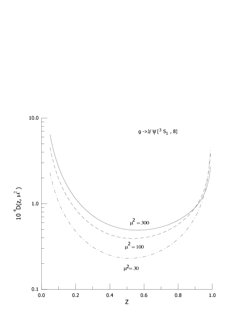
Figure 2: $D_{g\to J/\psi}(z,\mu^{2})$ at the $\mu^{2}$=30, 100 and 300 GeV² as a function of z.

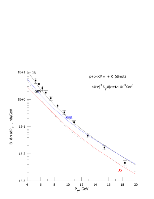
Figure 3: The spectrum of direct $J/\psi$ on $p_{T}$ at the $\sqrt{S}$=1800 GeV and $|\eta|<0.6$. The data points are from [1]. The $B$ is the $J/\psi$ lepton branching.

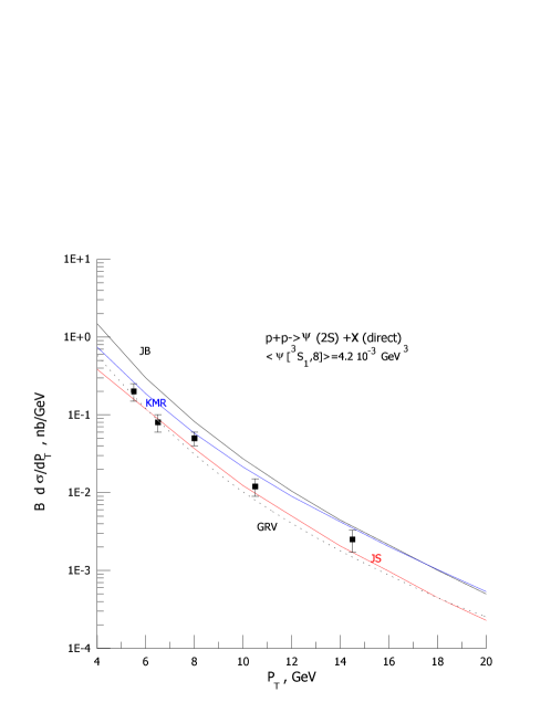
Figure 4: The spectrum of direct $\psi^{\prime}$ on $p_{T}$ at the $\sqrt{S}$=1800 GeV and $|\eta|<0.6$. The data points are from [1]. The $B$ is the $\psi^{\prime}$ lepton branching.

References

- (1) CDF Coll., F.Abe et al., Phys.Rev.Lett. 79, 572, (1997); ibib. 79, 578 (1997).
- (2) E.L.Berger and D.Jones, Phys.Rev. D23, 1521 (1981); R.Baier and R.Ruckl, Phys.Lett. B102, 364 (1981) ; S.S.Gershtein, A.K.Likhoded, S.R.Slabospiskii, Sov.J.Nucl.Phys. 34, 128 (1981).
- (3) G.T.Bodwin, E.Braaten, G.P.Lepage, Phys.Rev D51, 1125 (1995).
- (4) E.Braaten, T.C.Yuan, Phys.Rev. D50,3176 (1994); Phys.Rev. 52,6627 (1995); E.Braaten, K.Cheung, T.C.Yuan, Phys.Rev. 48,4230 (1993); E.Braaten, J.Lee, Nucl.Phys. 586,427 (2000); J.P.Ma, Nucl.Phys. 447,405 (1995).
- (5) L.V.Gribov, E.M.Levin, M.G.Ryskin, Phys.Rep. 100,1 (1983).
- (6) J.C.Collins and R.K.Ellis, Nucl.Phys. 360, 3 (1991).
- (7) S.Catani, M.Ciafoloni, F.Hautmann, Nucl.Phys. B366, 135 (1991).
- (8) V.S.Fadin, L.N.Lipatov, Nucl.Phys. B477, 767 (1996).
- (9) V.A.Saleev and N.P.Zotov, Mod.Phys.Lett. A9, 151 (1994).
- (10) V.A.Saleev, Phys.Rev. D65, 054041 (2002); V.A.Saleev, D.V.Vasin, Phys.Lett. B548, 161 (2002).
- (11) Ph.Hagler et al., Phys.Rev. 62, 071502 (2000); Phys.Rev.Lett. 86, 1446 (2001).
- (12) F.Yuan, K.-T.Chao, Phys.Rev. D63, 034006 (2001); F.Yuan et al., Phys.Rev.Lett. 87, 022001 (2001).
- (13) S.P.Baranov, Phys.Rev. D66, 114003 (2002).
- (14) E.Braaten, S.Fleming, Phys.Rev.Lett. 74, 3327 (1995).
- (15) E.Braaten, B.A.Kniehl, J.Lee, Phys.Rev. D62, 094005 (2000).
- (16) M.Kramer, Prog.Part.Nucl.Phys. 47, 141 (2001).
- (17) V.N. Gribov and L.N. Lipatov, Sov. J. Nucl. Phys. 15, 438 (1972) ; Yu.A. Dokshitser, Sov. Phys. JETP. 46, 641 (1977); G. Altarelli and G. Parisi, Nucl. Phys. B126, 298 (1977).
- (18) B.A.Kniehl, L.Zwirner, Preprint DESY 99-124; hep-ph/9909517.
- (19) E.Kuraev, L.Lipatov, V.Fadin, Sov. Phys. JETP 44, 443 (1976); Y.Balitskii and L.Lipatov, Sov. J. Nucl. Phys. 28, 822 (1978).
- (20) M.Gluck, E.Reya, A.Vogt, Z.Phys. C67, 433 (1995).
- (21) CTEQ Coll., H.L.Lai et al. Eur.Phys.J C12, 375 (2000).
- (22) J.Blumlein, DESY 95-121, (1995).
- (23) H. Jung, G. Salam, Eur. Phys. J. C19, 351 (2001).
- (24) M.A. Kimber, A.D. Martin and M.G. Ryskin, Phys. Rev. D63, 114027 (2001).
- (25) J.Kwiecinski, A.Martin, A.Stasto, Phys.Rev. D56, 3991 (1997).
- (26) M.Kraemer, Nucl.Phys. 459, 3 (1996).