Precision Electroweak Constraints on Hidden Local Symmetries

Abstract

In this talk we discuss the phenomenology of models with replicated electroweak gauge symmetries, based on a framework with the gauge structure $[SU(2){\ \rm or}\ U(1)]\times U(1)\times SU(2)\times SU(2)$.

1 Generalized BESS

In this talk we discuss the phenomenology of models with replicated electroweak gauge symmetries. The general framework we use is based on the gauge structure $[SU(2){\ \rm or}\ U(1)]\times U(1)\times SU(2)\times SU(2)$, and is conveniently illustrated in the figure below. This figure is drawn using “moose” notation,[1]

(1)

in which the circles represent gauge groups with the specified gauge coupling, and the solid lines represent separate $(SU(2)\times SU(2)/SU(2))$ nonlinear sigma model fields which break the gauged or global symmetries to which they are attached. The solid circles represent $SU(2)$ groups, with a “2” denoting a gauged $SU(2)$ and the “1” a global SU(2) in which only a U(1) subgroup has been gauged.

For convenience, the coupling constants of the gauge theories will be specified by

$$\tilde{g}^{\prime}={e\over\cos\theta\,\sin\phi}\,,\ \ g^{\prime}={e\over\cos\theta\,\cos\phi}\,,\ \ g={e\over\sin\theta\,\cos\omega}\,,\ \ \tilde{g}={e\over\sin\theta\,\sin\omega}\,,$$ (2)

and the $f$-constants (the analogs of $f_{\pi}$ in QCD) of the nonlinear sigma models by

$${f\over\sin\alpha}\,,\ \ v\,,\ \ {f\over\cos\alpha}~{}.$$ (3)

As we will see, the Lagrangian parameters $e$, $\theta$, and $v$, will be approximately equal to the electric charge, weak mixing angle, and Higgs expectation value in the one-doublet standard model. The scale $f$ sets the masses of the extra gauge bosons, and the theory reduces to the standard model in the limit $f\to\infty$, while the angle $\alpha$ allows us to independently vary the breaking of the duplicated $SU(2)$ or $U(1)$ gauge symmetries. Finally, the angles $\phi$ and $\omega$ determine the couplings of the gauge bosons which become massive at scale $f$.

The symmetry structure of this model is similar to that proposed in the BESS (Breaking Electroweak Symmetry Strongly) model,[2, 3] an effective Lagrangian description motivated by strong electroweak symmetry breaking. This model is in turn an application of “hidden local symmetry” to electroweak physics.[4] Accordingly, we refer to this paradigm as “generalized BESS.” The symmetry structure in the limit $f\to\infty$ is precisely that expected in a “technicolor” model,[5, 6] and the theory has a custodial symmetry in the limit $g^{\prime}$ and $\tilde{g}^{\prime}$ go to zero.

Generalized BESS is the simplest model of an extended electroweak gauge symmetry incorporating both replicated $SU(2)$ and $U(1)$ gauge groups. As such the electroweak sector of a number of models in the literature form special cases, including Noncommuting ETC,[7] topcolor,[8, 9] and electroweak $SU(3)$.[10, 11, 12] The general properties of precision electroweak constraints on these models[13, 14, 15] can correspondingly be viewed as special cases of what follows.[16]

2 Low-Energy Interactions

Constraints on models with extended electroweak symmetries arise both from low-energy and Z-pole measurements. The most sensitive low-energy measurements arise from measurements of the muon lifetime (which are used to determine $G_{F}$), atomic parity violation (APV), and neutrino-nucleon scattering. In the usual fashion, we may summarize the low-energy interactions in terms of four-fermion operators. The form of these interactions will depend, however, on the fermion charge assignments. For simplicity, in the remainder of this talk we consider models in which the fermion charge assignments are flavor universal. To illustrate the model-dependence of the results, we consider two examples.

First, we consider the case in which the ordinary fermions are charged only under the two groups at the middle of the moose

$$\lower 25.0pt\hbox{\includegraphics[width=170.71652pt]{G-BESS-Fermions1.eps}}\,.$$ (4)

In this case the charged current interactions may be computed to be

$${L}^{CC}=-\,{2\over v^{2}}\,J^{\mu+}J^{-}_{\mu}\,,$$ (5)

and the neutral current interactions

$${L}^{NC}=-\,{2\over v^{2}}(J^{\mu}_{3}-Q^{\mu}\,\sin^{2}\theta)^{2}-\,{2\cos^{2}\alpha\over f^{2}}\,\sin^{2}\theta\,\sin^{4}\omega\,Q^{\mu}Q_{\mu}~{}.$$ (6)

In these expressions, the currents $J^{\mu}_{\pm,3}$ and $Q^{\mu}$ are the conventional weak and electromagnetic currents. From these, we see that the strength of $G_{F}$, APV, and neutrino scattering is determined by $v$ in the usual way. Furthermore, comparing the two equations, we see that the strength of the charged and neutral current interactions, the so-called low-energy $\rho$ parameter, is precisely one (at tree-level). This last fact is a direct consequence of the Georgi-Weinberg neutral current theorem.[17]

As an alternative, consider the case in which the $SU(2)$ charges of the ordinary fermions arise from transforming under the gauge group at the end of the moose

$$\lower 25.0pt\hbox{\includegraphics[width=170.71652pt]{G-BESS-Fermions2.eps}}\,.$$ (7)

A calculation of the charged current interactions yields

$$L^{CC}=-2\left({1\over v^{2}}+{\cos^{2}\alpha\over f^{2}}\right)J^{\mu+}J^{-}_{\mu}\,,$$ (8)

while the neutral current interactions are summarized by

$${L}^{NC}=-\,{2\over v^{2}}(J^{\mu}_{3}-Q^{\mu}\,\sin^{2}\theta)^{2}-\,{2\cos^{2}\alpha\over f^{2}}\,(J^{\mu}_{3}-\sin^{2}\theta\cos^{2}\omega\,Q^{\mu})^{2}~{}.$$ (9)

Several points in this expression are of particular note: first, the value of $G_{F}$ as inferred from muon decay is no longer related simply to $v$. As we shall see in the next section, this ultimately will give rise to corrections to electroweak observables of order $(v/f)^{2}$ and unsuppressed by any ratios of coupling constants. Second, unlike the previous case, the strength of low-energy charged- and neutral-current interactions are no longer the same. It is interesting to note, however, that the strengths of the $J_{3}^{2}$ and $J^{+}J_{-}$ portions of the interactions are, however, the same – this is a reflection of the approximate custodial symmetry of the underlying model.

3 Z-Pole Constraints - General Structure

Many of the most significant constraints on physics beyond the standard model arise from precise measurements at the Z-pole. To interpret these measurements, we must compute the masses $W$ and $Z$ bosons and their couplings to ordinary fermions in terms of the Lagrangian parameters. For generalized BESS, we find the gauge-boson masses

$$M^{2}_{W}={e^{2}v^{2}\over 4\sin^{2}\theta}\left(1-\cos^{2}\alpha\sin^{4}\omega\,{v^{2}\over f^{2}}\right)+O\left({v^{4}\over f^{4}}\right)~{},$$ (10)

and

$$M^{2}_{Z}={e^{2}v^{2}\over 4\sin^{2}\theta\cos^{2}\theta}\left(1-(\cos^{2}\alpha\sin^{4}\omega+\sin^{2}\alpha\sin^{4}\omega)\,{v^{2}\over f^{2}}\right)+\ldots$$ (11)

From the expression for $M^{2}_{Z}$ and the calculations summarized in the previous section, we immediately see that there is a major difference in the structure of corrections to the standard model between cases I and II: corrections to the standard model relation between $G_{F}$, $\alpha$, $M^{2}_{Z}$, and the appropriately defined weak mixing angle $\sin^{2}\theta_{W}$ are generically of order $v^{2}/f^{2}$ in case II, but is of order $(\sin^{4}\omega,\ \sin^{4}\phi)v^{2}/f^{2}$ in case I. As a consequence, viewing the predictions of generalized BESS in terms of corrections to the corresponding standard model results, the corrections to standard model predictions in case I are (potentially) suppressed by ratios of coupling constants relative to the size of corrections in case II. This leads generically to weaker constraints in case I models.

In what follows, we will concentrate on models in the category of case I, in which the fermions are charged only under the gauge groups in the “middle” of the moose diagram. In order to make predictions for electroweak observables, we need to compute the couplings of the ordinary fermions to the light gauge boson eigenstates. In the case of the $W$ we find that the couplings to the left-handed fermions are

$${e\over\sin\theta}\left(1-\cos^{2}\alpha\,\sin^{4}\omega\,{v^{2}\over f^{2}}\right)+\ldots$$ (12)

and for the $Z$ we find the couplings

$${e\over\sin\theta\cos\theta}\left[1-(\sin^{2}\alpha\,\sin^{4}\phi+\cos^{2}\alpha\,\sin^{4}\omega)\,{v^{2}\over f^{2}}\right]\,T_{3}$$

$$-\,{e\over\sin\theta\cos\theta}\left(\sin^{2}\theta-\sin^{2}\alpha\,\sin^{4}\phi\,{v^{2}\over f^{2}}\right)\,Q~{}.$$ (13)

Comparing to the computed gauge-boson masses we see that, for case I, all corrections to standard model predictions may be expressed in terms of two combinations of Lagrangian parameters:

$$c_{1}=\cos^{2}\alpha\,\sin^{4}\omega\,{v^{2}\over f^{2}}\,,\ \ \ \ \ c_{2}=\sin^{2}\alpha\,\sin^{4}\phi\,{v^{2}\over f^{2}}~{}.$$ (14)

This allows us to compute bounds on model parameters in terms of fits to $c_{1}$ and $c_{2}$, greatly simplifying the calculations.

Finally, while we will not explicitly display the results in case II, a similar calculation shows that corrections to gauge-boson couplings in this case are proportional to $(\sin^{2}\omega,\ \sin^{2}\phi)v^{2}/f^{2}$.

4 Flavor-Universal Results

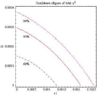
Figure 1: Constraints on $c_{1}$ and $c_{2}$ at the 68%, 95%, and 99% confidence level based on fits to precision electroweak data.[19]

From the calculations above, we may compute the values of all precisely measured electroweak quantities in terms of the Lagrangian parameters given above. Using the procedure outlined in Burgess et. al.,[18] we perform fits to the electroweak observables listed in the most recent compilation by the LEP Electroweak Working Group,[19] which include Z-pole observables as well as the width of the $W$ boson, and low-energy atomic parity violation and neutrino-nucleon scattering. The 68%, 95%, and 99% confidence level fits for the parameters $c_{1,2}$ is shown in Figure 1.

For a given value of $\alpha$, we may unfold these constraints to produce a 95% lower bound on $f$ in terms of $\sin\omega$ and $\sin\phi$. A sense of the reach of these bounds is given in Figure 2, plotted for $\alpha=\pi/4$. For typical values of $\sin\phi$ and $\sin\omega$, the bounds on the scale $f$ range from a few TeV.

Many of the models cited above correspond to the extra gauge groups being weak, $\sin\phi$ or $\sin\omega$ of order 1, in which case the bounds on $f$ are of order 10 TeV.[13, 14, 15] Formally the corrections vanish when the couplings of the extra gauge groups become strong, that is in the limit $\sin\phi\,,\sin\omega\to 0$. The phenomenologically interesting question is whether there are any interesting models corresponding to this case, in which case there may be interesting structure at relatively low scales!

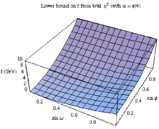
Figure 2: The lower-bound on $f$ at 95% confidence level for $\alpha=\pi/4$, as a function of $\sin\omega$ and $\sin\phi$, based on fits to precision electroweak data.[19]

References

- [1] H. Georgi, Nucl. Phys. B 266, 274 (1986).
- [2] R. Casalbuoni, S. De Curtis, D. Dominici and R. Gatto, Phys. Lett. B 155, 95 (1985).
- [3] R. Casalbuoni, A. Deandrea, S. De Curtis, D. Dominici, R. Gatto and M. Grazzini, Phys. Rev. D 53, 5201 (1996) [arXiv:hep-ph/9510431].
- [4] M. Bando, T. Kugo and K. Yamawaki, Phys. Rept. 164, 217 (1988).
- [5] S. Weinberg, Phys. Rev. D 13, 974 (1976).
- [6] S. Weinberg, Phys. Rev. D 19, 1277 (1979).
- [7] R. S. Chivukula, E. H. Simmons and J. Terning, Phys. Lett. B 331, 383 (1994) [arXiv:hep-ph/9404209].
- [8] C. T. Hill, Phys. Lett. B 266, 419 (1991).
- [9] C. T. Hill, Phys. Lett. B 345, 483 (1995) [arXiv:hep-ph/9411426].
- [10] F. Pisano and V. Pleitez, Phys. Rev. D 46, 410 (1992) [arXiv:hep-ph/9206242].
- [11] P. H. Frampton, Phys. Rev. Lett. 69, 2889 (1992).
- [12] S. Dimopoulos and D. E. Kaplan, Phys. Lett. B 531, 127 (2002) [arXiv:hep-ph/0201148].
- [13] R. S. Chivukula, E. H. Simmons and J. Terning, Phys. Rev. D 53, 5258 (1996) [arXiv:hep-ph/9506427].
- [14] R. S. Chivukula and J. Terning, Phys. Lett. B 385, 209 (1996) [arXiv:hep-ph/9606233].
- [15] C. Csaki, J. Erlich, G. D. Kribs and J. Terning, Phys. Rev. D 66, 075008 (2002) [arXiv:hep-ph/0204109].
- [16] R. S. Chivukula, H. J. He, J. Howard, and E. H. Simmons, work in progress.
- [17] H. Georgi and S. Weinberg, Phys. Rev. D 17, 275 (1978).
- [18] C. P. Burgess, S. Godfrey, H. Konig, D. London and I. Maksymyk, Phys. Rev. D 49, 6115 (1994) [arXiv:hep-ph/9312291].
- [19] LEP Electroweak Working Group, arXiv:hep-ex/0212036.