Analysis of energy- and time-dependence
of supernova shock effects on neutrino crossing probabilities

Abstract

It has recently been realized that supernova neutrino signals may be affected by shock propagation over a time interval of a few seconds after bounce. In the standard three-neutrino oscillation scenario, such effects crucially depend on the neutrino level crossing probability $P_{H}$ in the 1-3 sector. By using a simplified parametrization of the time-dependent supernova radial density profile, we explicitly show that simple analytical expressions for $P_{H}$ accurately reproduce the phase-averaged results of numerical calculations in the relevant parameter space. Such expressions are then used to study the structure of $P_{H}$ as a function of energy and time, with particular attention to cases involving multiple crossing along the shock profile. Illustrative applications are given in terms of positron spectra generated by supernova electron antineutrinos through inverse beta decay.

I Introduction

The realization that the supernova shock propagation can affect neutrino flavor transitions Schi a few seconds after core bounce Wils is gaining increasing attention in the recent literature on supernova neutrinos Raff ; Beac ; Lead ; Reli ; Spin ; Shoc ; Chou ; Luna . Indeed, time-dependent variations of the neutrino potential in matter Matt along the supernova shock profile can leave an interesting imprint on the energy and time structure of the (anti)neutrino signal at the Earth Schi ; Shoc ; Luna . Observation of such possible effects, although very challenging from an experimental viewpoint, would open a unique opportunity to study some aspects of the supernova shock dynamics in “real time.” Moreover, the strong sensitivity of such effects to the neutrino oscillation parameters Schi ; Shoc ; Luna might, in principle, provide us with additional constraints (or hints, at least) on the neutrino mass spectrum and mixing angles.

From a conservative viewpoint, it should be stressed that current simulations of core-collapse supernovae, despite remarkable efforts, may still require substantial physics improvements Jank . It is not excluded that more refined simulations might significantly modify, e.g., the main features of shock profile discussed in Schi , and especially its propagation velocity and density gradient, which govern the structure of the neutrino crossing probabilities Schi ; Shoc ; Luna . Moreover, the time and energy dependence of the source (anti)neutrino fluxes might be more complicated and uncertain Unce ; Flux than is customarily assumed, making it more difficult to identify shock-related signals. All these potential systematic uncertainties in the basic physics ingredients might be large enough to weaken the significance of shock-related signals, even with hypothetically large experimental statistics. However, despite all these caveats, the stakes are so high that further investigations on possible shock effects on supernova neutrinos are widely justified, in our opinion.

The purpose of this work is to investigate in some detail the energy- and time-dependence of the neutrino crossing probabilities along the supernova shock. We assume the active $3\nu$ oscillation scenario (Sec. II), and construct an empirical parameterization for the shock profile (Sec. III). Analytical calculations are shown to reproduce well (and to be much more convenient than) numerical approaches to the overall crossing probabilities, and are used to break down the multiple transition structure along the shock density profile, both in the energy domain (Sec. IV) and in the time domain (Sec. V). Finally, applications are given in terms of antineutrino event spectra observable at the Earth through inverse beta decay (Sec. VI). Conclusions and prospects for further work are given in Sec. VII.

The bottom line of our work is that simple, analytical calculations of the crossing probabilities along the supernova shock profile appear to be adequate to study the structure of neutrino flavor transitions in the energy and time domain, for all practical purposes. The specific probability values estimated in this work, however, should not be taken too literally, being based on a simplified description of the matter density profile, which is subject to change as more detailed supernova shock simulations are performed and become publicly available.

II $3\nu$ notation and analytical approximations

Throughout this work, we consider only flavor transitions among the three known active neutrinos $\nu_{e}$, $\nu_{\mu}$, and $\nu_{\tau}$. In the following, we set the notation and briefly describe the analytical expressions for the crossing probabilities.

II.1 Notation for $3\nu$ kinematics and dynamics

The $3\nu$ squared mass spectrum is parameterized as

$$(m^{2}_{1},\,m^{2}_{2},\,m^{2}_{3})=\left(-\frac{\delta m^{2}}{2},\,+\frac{\delta m^{2}}{2},\,\pm\Delta m^{2}\right)\ ,$$ (1)

where the sign before $\Delta m^{2}$ distinguishes the cases of normal ($+$) and inverted ($-$) hierarchy. The mixing matrix $U$ is defined in terms of three rotation angles $\theta_{ij}$, ordered as for the quark mixing matrix Hagi ,

$$U=U(\theta_{12},\,\theta_{13},\,\theta_{23}).$$ (2)

When needed, we take

$$\delta m^{2}/\mathrm{eV}^{2} = 7.3\times 10^{-5}\ ,$$ (3)

$$\sin^{2}\theta_{12} = 0.315\ ,$$ (4)

corresponding to the so-called LMA-I best fit to the solar and reactor neutrino data LMAI . We also take

$$\Delta m^{2}=3\times 10^{-3}\mathrm{\ eV}^{2}\ ,$$ (5)

close to the best fit to the atmospheric and accelerator neutrino data detected in Super-Kamiokande Deco . The value of $\sin^{2}\theta_{23}$ is basically irrelevant for supernova neutrinos, since it corresponds to an unobservable rotation in the $(\nu_{\mu},\nu_{\tau})$ flavor subspace. Concerning the mixing parameter $\sin^{2}\theta_{13}$, we will pick up several representative values, well below the current $3\sigma$ upper limit ($\sin^{2}\theta_{13}<0.05$ Deco ).

The mass gap hierarchy ($\delta m^{2}/\Delta m^{2}\ll 1$) and the smallness of $\sin^{2}\theta_{13}$ guarantee, to a very good approximation, the factorization of the $3\nu$ neutrino dynamics into a “low” ($L$) and a “high” ($H$) $2\nu$ subsystem, whose dominant oscillation parameters are $(\delta m^{2},\,\theta_{12})$ and $(\Delta m^{2},\,\theta_{13})$, respectively (see KuPa ; Ours and references therein). The corresponding neutrino wavenumbers are defined as

$$k_{L} = \delta m^{2}/2E\ ,$$ (6)

$$k_{H} = \Delta m^{2}/2E\ ,$$ (7)

where $E$ is the neutrino energy.

Potentially large matter effects Matt are expected when either $k_{L}$ or $k_{H}$ take values close to the neutrino potential $V$ in matter,

$$V=\sqrt{2}\,G_{F}\,N_{e}(x)\ ,$$ (8)

where $N_{e}$ is the electron density at the supernova radius $x$. In appropriate units,

$$\frac{V(x)}{\mathrm{eV}^{2}/\mathrm{MeV}}=7.6\times 10^{-8}\,Y_{e}\,\frac{\rho(x)}{\mathrm{g/cm}^{3}}\ ,$$ (9)

where $Y_{e}$ is the electron/nucleon number fraction (that we assume equal to 1/2), while $\rho(x)$ is the radial mass density profile. We conventionally take $k_{L}$, $k_{H}$, and $V$ to be positive (as in Ref. Ours ), irrespective of the neutrino type ($\nu$ or $\overline{\nu}$) and hierarchy (normal or inverted).

The $V(x)$ profile in supernovae is often approximated by a static power law, $V(x)\sim x^{-n}$ with $n\sim 3$. In the presence of a shock wave, however, such static profile can be significantly modified Schi ; Wils . In particular the shock wave, while propagating outwards at supersonic speed, leaves behind a rarefaction zone, followed by a high-density region and by a sharp drop of density (down to the static value) at

$$x_{s}=\mathrm{shock\ front\ radius}\ .$$ (10)

This abrupt change of density occurs over a microscopic length scale governed by the mean free path of ions and electrons, which, for our purposes, can be effectively taken as zero. Correspondingly, at $x=x_{s}$ the matter potential $V(x)$ drops from

$$V^{+}=\lim_{x\to x_{s}^{-}}V(x)$$ (11)

to

$$V^{-}=\lim_{x\to x_{s}^{+}}V(x)\ ,$$ (12)

with a typical ratio Schi

$$\xi=\frac{V^{+}}{V^{-}}\simeq 10\ .$$ (13)

Given the peculiar step-like features of the matter potential at the shock front, in the following we discuss the analytical expressions of the crossing probabilities for $x\neq x_{s}$ and $x=x_{s}$ separately. We then study the general case of multiple crossings along the neutrino trajectory.

II.2 Crossing probability at $x\neq x_{s}$

As previously mentioned, potentially large matter effects are expected when $k_{L,H}\sim V$. In particular, if the condition

$$V(x_{H})=k_{H}$$ (14)

occurs at some point $x_{H}(\neq x_{s})$, there is a finite probability $P_{H}$ of crossing between effective mass eigenstates in the $H$ subsystem, which is given to a good approximation by the so-called double exponential formula Petc

$$P_{H}=\frac{\exp(2\pi r_{H}k_{H}\cos^{2}\theta_{13})-1}{\exp(2\pi r_{H}k_{H})-1}\$$ (15)

for both neutrinos and antineutrinos (see Ours and related bibliography therein), with

$$r_{H}=\left|\frac{d\ln V(x)}{dx}\right|^{-1}_{x=x_{H}}\ .$$ (16)

For all the $V(x)$ profiles and $\sin^{2}\theta_{13}$ values that will be used in the following, the above formula reduces to the well-known Landau-Zener (LZ) limit

$$P_{H}\simeq\exp(-2\pi r_{H}k_{H}\sin^{2}\theta_{13})\ ,$$ (17)

at any $\nu$ energy of practical interest.

In principle, the occurrence of the condition $k_{L}=V(x_{L})$ at some radius $x_{L}$ could also induce neutrino level crossing in the $L$ subsystem with probability $P_{L}$ (generally different for neutrinos and antineutrinos; see, e.g., Digh ; Ours ). However, for $\sin^{2}\theta_{12}$ as large as in Eq. (4) it turns out that the $L$-transition is adiabatic,

$$P_{L}(\nu)\simeq 0\simeq P_{L}(\overline{\nu})\ ,$$ (18)

at all points $x\neq x_{s}$.

II.3 Crossing probability at $x=x_{s}$

The analytical approximations in Eqs. (17) and (18) break down at $x=x_{s}$, where the density gradient explodes (and $r_{H}\to 0$). In this case, the crossing probability $P_{s}$ is determined by the conservation of flavor across the $V(x)$ discontinuity, with the well-known result (see, e.g., KuPa ):

$$P_{s}=\sin^{2}(\theta_{m}^{+}-\theta_{m}^{-})\ ,$$ (19)

where $\theta_{m}^{+}$ and $\theta_{m}^{-}$ are the effective mixing angles in matter immediately before $(V=V^{+})$ and after $(V=V^{-})$ the shock front position $x_{s}$, respectively. For the $H$ transition, such angles are defined by

$$\cos 2\theta_{m}^{\pm}=\frac{\cos 2\theta_{13}-V^{\pm}/k_{H}}{\sqrt{(\cos 2\theta_{13}-V^{\pm}/k_{H})^{2}+(\sin 2\theta_{13})^{2}}}\ ,$$ (20)

for both neutrinos and antineutrinos. In the limit of very small $\theta_{13}$, the above equations imply $P_{s}\simeq 1$ for $k_{H}\in[V^{-},V^{+}]$, and $P_{s}\simeq 0$ otherwise. Notice that the extremely nonadiabatic limit $P_{s}\simeq 1$ would also be obtained from Eq. (15) for $\theta_{13}\to 0$ and $r_{H}\to 0$. However, the tempting approximation $P_{s}=1$ (for $k_{H}\in[V^{-},V^{+}]$) does not work well for $\sin^{2}\theta_{13}$ as large as $O(10^{-3})$–$O(10^{-2})$, the “top-hat” behavior for $P_{s}$ being significantly smeared out [i.e., a tail $P_{s}\neq 0$ is developed for $k_{H}$ outside the range $[V^{-},V^{+}]$, especially for $k_{H}\stackrel{{\scriptstyle\textstyle<}}{{\raisebox{-2.58334pt}{$\sim$}}}V^{-}$, as easily understandable on the basis of Eq. (20)]. Therefore, we adopt the exact Eqs. (19) and (20) to calculate the $H$ crossing probability at the shock front, without further approximations.

Concerning the analogous crossing probability in the $L$ sector, similar expressions apply, modulo the substitutions $\theta_{13}\to\theta_{12}$ and $k_{H}\to k_{L}$ in Eqs. (19) and (20). The strong nonadiabatic character of the transition at the shock front can now lead to $P_{L}\neq 0$ in some corners of the parameter space [in contrast to Eq. (18)]. However, as we shall discuss at the end of Sec. IV C, such parameter values happen to have little phenomenological relevance. Therefore, unless otherwise noted, we shall formally take $P_{L}\simeq 0$ not only for $x\neq x_{s}$ [Eq. (18)], but also for $x=x_{s}$.

II.4 Analytical expressions for multiple crossings

For $P_{L}\simeq 0$, the formal expression for the $\nu_{e}$ survival probability $P_{ee}$ Digh ; Ours is exceedingly simple (up to Earth matter effects):

$$P_{ee}\simeq\left\{\begin{array}[]{ll}\sin^{2}\theta_{12}\,P_{H}&(\nu,\;\mathrm{normal}),\\ \cos^{2}\theta_{12}&(\overline{\nu},\;\mathrm{normal}),\\ \sin^{2}\theta_{12}&(\nu,\;\mathrm{inverted}),\\ \cos^{2}\theta_{12}\,P_{H}&(\overline{\nu},\;\mathrm{inverted}),\\ \end{array}\right.$$ (21)

where “normal” and “inverted” refer to the hierarchy type. In the above equation, we have neglected small additive terms of $O(\sin^{2}\theta_{13})$, which are not relevant for our discussion. From the above equations, it appears that $P_{H}$ can modulate the (otherwise constant) survival probability of $\nu_{e}$ in normal hierarchy and of $\overline{\nu}_{e}$ in inverted hierarchy, thus providing an important handle to solve the current hierarchy ambiguity.

In the presence of a propagating shock wave, the calculation of $P_{H}$ is not entirely trivial. For the shock profiles studied in Schi ; Shoc , the condition in Eq. (14) can occur at up to three points $x_{i}\neq x_{s}\ (i=1,2,3)$:

$$V(x_{i})=k_{H}\ (i=1,2,3)\ ,$$ (22)

In the most general case, two such points belong to the rarefaction zone ($x_{1}<x_{2}<x_{s}$) and one to the static region below the shock front $(x_{3}>x_{s})$. The corresponding crossing probabilities are denoted as $P_{1}$, $P_{2}$, and $P_{3}$. The $P_{i}$’s can be analitically calculated as in Eq. (17), with the inverse log-derivative $r_{i}$ [Eq. (16)] evaluated at the point $x_{i}$. In addition, one should consider the crossing probability $P_{s}$ at $x=x_{s}$, as given by Eqs. (19) and (20). Therefore, the global $P_{H}$ must be generally constructed in terms of four crossing probabilities $P_{1}$, $P_{2}$, $P_{s}$, and $P_{3}$, occurring at the points

$$x_{1}<x_{2}<x_{s}<x_{3}\ ,$$ (23)

respectively.

If we assume that all relative neutrino phases can be averaged away, and that the four transitions can be exactly factorized, the overall crossing probability $P_{H}$ can be defined in terms of a simple matrix equation KuPa

$$\left(\begin{array}[]{cc}1-P_{H}&P_{H}\\ P_{H}&1-P_{H}\end{array}\right)=\prod_{i=1,2,s,3}\left(\begin{array}[]{cc}1-P_{i}&P_{i}\\ P_{i}&1-P_{i}\end{array}\right)\ ,$$ (24)

whose solution is

$$P_{H} = P_{1}+P_{2}+P_{s}+P_{3}-2(P_{1}P_{2}+P_{1}P_{s}+P_{1}P_{3}+P_{2}P_{s}+P_{2}P_{3}+P_{s}P_{3})$$ (25)

$$+4(P_{1}P_{2}P_{s}+P_{1}P_{2}P_{3}+P_{1}P_{s}P_{3}+P_{2}P_{s}P_{3})-8P_{1}P_{2}P_{s}P_{3}\ .$$

We will refer to this simple equation for our analytical calculations of $P_{H}$.

Although the smallness of $\theta_{13}$ implies that each of the four transitions $P_{1,2,s,3}$ is (in general) well localized and can thus be separated from the others, the intrinsic accuracy of the factorization in Eq. (24) is not obvious a priori in the whole relevant parameter space. There are zones of the shock profile where two transition points can become very close and eventually merge, or where the local density shape can be strongly different from the static, quasi-cubic power law which was used in Ours to test the analytical recipe in of Eq. (15). Moreover, in the presence of multiple (interfering) transition amplitudes, it is worth checking that reasonable phase averaging effectively reproduces the incoherent factorization implicit in Eq. (24).

For such reasons, we think it is useful to compare the analytical calculations of $P_{H}$ [based on Eqs. (16) and (17) for $x=x_{1,2,3}$, and on Eqs. (19) and (20) for $x=x_{s}$] with the results of a numerical (Runge-Kutta) evolution of the neutrino flavor propagation equations along representative shock density profiles. To our knowledge, such reassuring comparison has not been explicitly performed in the available literature. In order to do so in both the time and energy domain (Secs. IV and V, respectively), we need a parameterization of the shock wave profile which is (almost everywhere) continuous in both the radius $x$ and in post-bounce time $t$. Unfortunately, a similar parameterization (or, equivalently, a dense numerical table) is not publicly available; only some representative profiles are graphically reported in Schi and Shoc . Moreover, only the profiles in Schi exhibit (by construction) the correct step-like profile at $x=x_{s}$. In the following section, we thus introduce a simplified parametrization of the supernova density profile which is continuous in the $(x,t)$ variables [excepting the shock-front discontinuity point]. Such empirical profile captures the main qualitative features of the time and radial dependence of the (supposed spherically symmetric) shock propagation, allowing us to perform a meaningful comparison of numerical and analytical results, and to break down explicitly the analytical calculation of $P_{H}$ into its four components $P_{1}$, $P_{2}$, $P_{s}$, and $P_{3}$. Needless to say, such a simplified profile can and must be improved when more informative or refined supernova shock simulations become available.

A final remark is in order. In this work we are mainly concerned with the factorization of transition within the $H$ subsystem, since the factorization between the $L$ and $H$ subsystems is guaranteed for $\delta m^{2}$ as low as in Eq. (3). However, small corrections to the $L$-$H$ factorization might arise for values of $\delta m^{2}\sim\mathrm{few}\times 10^{-4}$ eV², not considered here (see, e.g., KuPa for earlier discussions and Luna ; LimS for more recent considerations). The analysis of these possible small corrections is beyond the scope of this work.

III Empirical parametrization of the Shock density profile

In this section we introduce a simplified, empirical parametrization of the shock density profile $\rho$, which reproduces the main features of the graphical profile in Schi and, at same time, is continuous in both $x$ and $t$ [excepting the case $x(t)=x_{s}(t)$]. In this way, numerical and analytical calculations of $P_{H}$ can continuously cover the relevant parameter space.

For post-bounce times $t\stackrel{{\scriptstyle\textstyle<}}{{\raisebox{-2.58334pt}{$\sim$}}}1\,\mathrm{s}$, shock effects Schi ; Shoc take place typically at $V>k_{H}$ and do not significantly affect the $H$ subsystem. The density profile can thus be effectively approximated by its static limit $\rho_{0}$ as taken from Schi :

$$t\stackrel{{\scriptstyle\textstyle<}}{{\raisebox{-2.58334pt}{$\sim$}}}1\,\mathrm{s}\ \ \Rightarrow\ \ \frac{\rho_{0}(x)}{\mathrm{g/cm}^{3}}\simeq 10^{14}\,\left(\frac{x}{\mathrm{km}}\right)^{-2.4}\ .$$ (26)

For post-bounce times $t\stackrel{{\scriptstyle\textstyle>}}{{\raisebox{-2.58334pt}{$\sim$}}}1\,\mathrm{s}$, the condition $V\sim k_{H}$ can be fulfilled, and the shock profile can thus modulate $P_{H}$. We characterize the profile in terms of the shock front position $x_{s}$ and of its shape variation $f(x)$ (with respect to $\rho_{0}$) for $x\leq x_{s}$. Formally, one can write

$$t\stackrel{{\scriptstyle\textstyle>}}{{\raisebox{-2.58334pt}{$\sim$}}}1\,\mathrm{s}\ \ \Rightarrow\ \ \rho(x)=\rho_{0}(x)\cdot\left\{\begin{array}[]{ll}\xi\cdot f(x)&,\;x\leq x_{s}\ ,\\ 1&,\;x>x_{s}\ ,\end{array}\right.$$ (27)

where $\xi$ (the matter density enhancement at $x=x_{s}$) has been defined in Eq. (13) (see also Schi ).

In Eq. (27), the function $f(x)$ parametrizes the rarefaction zone (“hot bubble”) above the shock front, characterized by a drop of density over more than one decade in $x$, and by an asymptotic density increase for $x\ll x_{s}$. After some trials, we have chosen the following (purely empirical) parametrization for $f(x)$, which reproduces the main features of the graphical profiles in Schi :

$$\ln f(x)=\left[0.28-0.69\ln(x_{s}/\mathrm{km})\right]\cdot\left[\arcsin(1-x/x_{s})\right]^{1.1}\ ,$$ (28)

In the above equations we assume (following Schi ) a slightly accelerating shock-front position $x_{s}$,

$$x_{s}(t)=x^{0}_{s}+v_{s}\,t+\frac{1}{2}\,a_{s}\,t^{2}\ ,$$ (29)

with parameters approximately given by

$$x^{0}_{s} \simeq -4.6\times 10^{3}\mathrm{\ km}\ ,$$ (30)

$$v_{s} \simeq 11.3\times 10^{3}\mathrm{\ km/s}\ ,$$ (31)

$$a_{s} \simeq 0.2\times 10^{3}\mathrm{\ km/s}^{2}\ .$$ (32)

Notice that: ($i$) The time dependence of $\rho(x)$ in Eq. (27) is implicit, through the function $x_{s}=x_{s}(t)$; and ($ii$) at small radii, it is

$$x\ll x_{s}\ \ \Rightarrow\ \ \rho(x)\simeq\rho_{0}(x)\times 16\,(x_{s}/\mathrm{km})^{-1.13}\ .$$ (33)

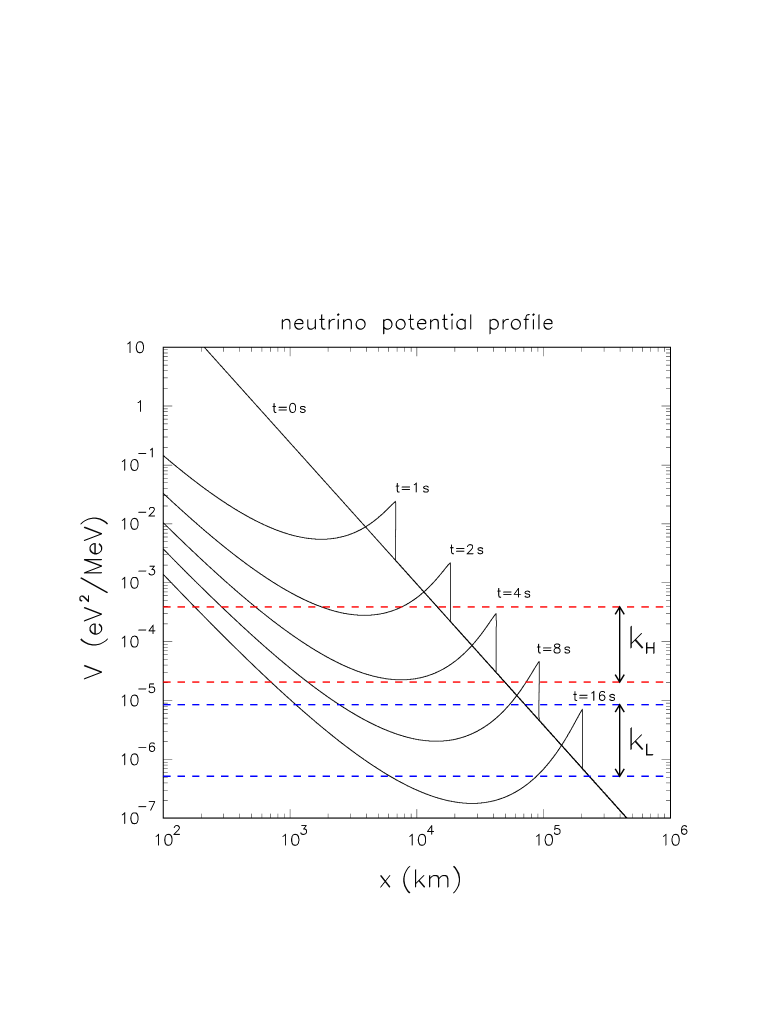
Figure 1: Neutrino potential $V$ as a function of the supernova radius $x$, for different values of the post-bounce time $t$, as derived from our simplified parametrization of the profiles in Schi . The horizontal bands represent typical ranges of the neutrino wavenumbers $k_{H}$ and $k_{L}$. See the text for details.

Figure 1 shows the neutrino potential $V(x)$ as derived from the above parametrization [Eqs.(26)–(32)] for representative post-bounce times $\geq 1$ s, as well as for the static profile $(t\simeq 0)$. These curves reasonably reproduce the main features of the shock profiles from Schi . The horizontal bands represent the ranges where the neutrino potential equals the two wavenumbers ($k_{H}=V$ and $k_{L}=V$), for a representative energy interval $E\in[4,\,70]$ MeV.

As previously mentioned, a line at constant $k_{H}$ can intersect the $V(x)$ profile in Fig. 1 in at most three points $x_{i}$, ordered as $x_{1}\leq x_{2}\,(\leq x_{s})\leq x_{3}$, and corresponding to level crossing probabilities $P_{1}$, $P_{2}$, and $P_{3}$. A further crossing probability $P_{s}$ is related to the step-like feature of the profile at the shock front $x=x_{s}$. Two of the four critical points ($x_{1},x_{2},x_{s},x_{3}$) can merge in the following cases: (1) at the bottom of the rarefaction zone (denoted as $x_{r}$), where $x_{1}=x_{2}$; (2) at the shock front $(x_{s})$, where it is $x_{2}=x_{s}$ for $V^{+}=k_{H}$ or $x_{3}=x_{s}$ for $V^{-}=k_{H}$. Single transitions can instead occur at early times or high energies ($V(x)=k_{H}$ at $x=x_{3}$ only), as well as at late times or low energies ($V(x)=k_{H}$ at $x=x_{1}$ only). Therefore, the three critical cases $V(x_{r})=k_{H}$ ($x_{1}=x_{2}$) and $V^{\pm}=k_{H}$ ($x_{2,3}=x_{s}$) are expected to mark significant changes in the behavior of $P_{H}$.

We conclude this section with a few cautionary remarks. At present, the detailed shape of $V(x)$ at the shock front is poorly known, since the physical requirement of a density discontinuity at $x=x_{s}$ is implemented “by hand” Schi , as a necessary correction to the artificially smooth profile from simulations Shoc . A side effect of the shock front steepening is the appearance of a local “cusp” at $x=x_{s}$ (as apparent in Ref. Schi and even more in our Fig. 1), which might well be unphysical. However, we do not smooth it out, since it actually provides us with a useful, nontrivial check of numerical versus analytical calculations of $P_{H}$ in an “extreme” condition (i.e., around a sudden change in the sign and value of the density gradient). Finally, we observe that some “leftover” turbulence might be expected in the rarefaction zone behind the shock front, inducing fuzzy variations of the local density. Such variations might lead to more than three solutions of Eq. (22) in some cases, and thus to a more complicated and “random” structure for $P_{H}$. This possibility (not considered in this work) should be kept in mind when more refined supernova shock simulations will become available.

IV Analysis of crossing probabilities in the energy domain

In this Section we study in detail the energy dependence of $P_{H}$ at fixed time. We pay particular attention to the discussion of multiple transitions along the shock density profile.

IV.1 Analytical vs numerical calculations of $P_{H}(E)$

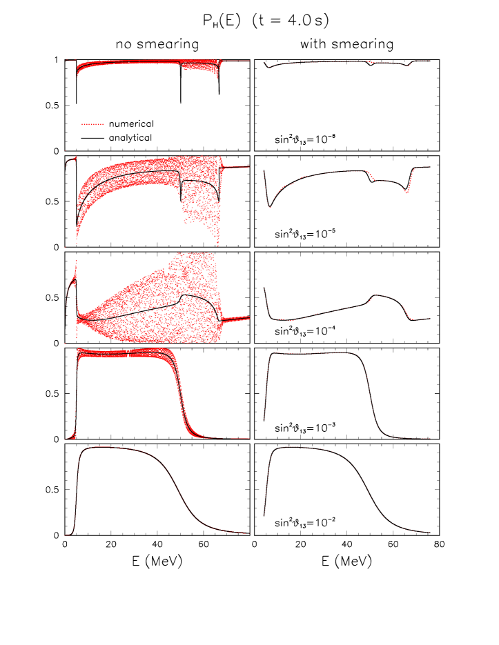
Figure 2: Comparison of numerical and analytical calculations of the crossing probability $P_{H}(E)$ (dots and solid curves, respectively) at $t=4\,\mathrm{s}$ and for five representative values of $\sin^{2}\theta_{13}$. In the right panels, phase effects are energy-averaged.

Figure 2 shows our calculation of $P_{H}(E)$ at fixed post-bounce time $t=4\,\mathrm{s}$, for five representative values of $\sin^{2}\theta_{13}$, ranging from $10^{-6}$ (top) to $10^{-2}$ (bottom). In the left panels, a direct comparison is made between analytical calculations (solid curves) and Runge-Kutta numerical calculations (dots), performed at $5\times 10^{3}$ equally-spaced points in the interval $E\in[0,80]$ MeV. In general, up to four energy regimes can be identified, with significant changes at the three critical energies $E\simeq 5$, 50, and 67 MeV. These energies fulfill (for the $V(x)$ profile at $t=4$ s) the three critical conditions $k_{H}=V^{+},V^{-},V(x_{r})$ which, as discussed in the previous section, signal the merging of two of the four possible level crossing points.

In the left panel of Fig. 2, the results of the numerical calculations appear to be generally scattered around the analytical curve. The reason is that Runge-Kutta calculations keep track of the phase(s) of the level crossing amplitude(s), while our analytical approximations average out this information from the beginning. For a single numerical amplitude, the associated phase becomes ineffective after taking the squared modulus. For multiple (interfering) amplitudes, instead, the relative phases do provide an oscillating structure in $P_{H}$, which is apparent in the numerical results.

In the right panels of Fig. 2, the oscillating structure of the numerical results is averaged out by a convolution with a Gaussian function (with one-sigma width of $\pm 1$ MeV), which simulates a generic “smearing” process (e.g., experimental energy resolution). The same convolution is applied to the analytical results. It can be seen that there is very good agreement between the two different (numerical and analytical) approaches after smearing. The results of Fig. 2 (and of other checks that we have performed for different post-bounce times) show that analytical calculations of $P_{H}$ coincide with phase-averaged numerical results with very good accuracy, even close to the “critical” points where two transitions collapse. Moreover, analytical calculations are actually much more convenient than the numerical ones, which require a very high sampling rate in order to perform efficient phase-averaging and to prevent numerical artifacts.

Let us now discuss in more detail the behavior of the analytical $P_{H}$ in the left panels of Fig. 2. We remind that $P_{s}$ [the crossing probability at the shock front, Eq. (19)] has almost a top-hat behavior: it rapidly drops from $\sim 1$ to zero for $k_{H}$ outside the range $[V^{-},V^{+}]$, i.e., for $E$ outside the range $[5,50]$ MeV (for the specific profile used in Fig. 2). This behavior depends only mildly on $\sin^{2}\theta_{13}$ [as far as it is $\stackrel{{\scriptstyle\textstyle<}}{{\raisebox{-2.58334pt}{$\sim$}}}O(10^{-2})$]. The LZ probabilities $P_{1,2,3}$ are instead exponentially suppressed as $\sin^{2}\theta_{13}$ increases [see Eq. 15]. In particular, in the bottom panels of Fig. 2 ($\sin^{2}\theta_{13}=10^{-3}$ and $10^{-2}$), $P_{H}$ is dominated by $P_{s}$ (with its characteristic top-hat behavior), with very little contributions from $P_{1,2,3}$. The dominance of a single crossing amplitude in $P_{H}$ explains the suppression of the numerical oscillations in the same panels.

Conversely, for $\sin^{2}\theta_{13}$ as small as $10^{-6}$ eV² (top panel in Fig. 2), the probabilities $P_{1,2,3}$ (as well as $P_{s}$) can all become as large as $\sim 1$, rendering $P_{H}\simeq 1$. In particular, for $E\stackrel{{\scriptstyle\textstyle<}}{{\raisebox{-2.58334pt}{$\sim$}}}5$ MeV, only $P_{1}\simeq 1$ is active (single crossing, well above the shock front). For $5\stackrel{{\scriptstyle\textstyle<}}{{\raisebox{-2.58334pt}{$\sim$}}}E\stackrel{{\scriptstyle\textstyle<}}{{\raisebox{-2.58334pt}{$\sim$}}}50$ MeV, besides $P_{s}\simeq 1$ it is also $P_{1,2}\simeq 1$ (two crossings in the rarefaction zone). For $50\stackrel{{\scriptstyle\textstyle<}}{{\raisebox{-2.58334pt}{$\sim$}}}E\stackrel{{\scriptstyle\textstyle<}}{{\raisebox{-2.58334pt}{$\sim$}}}67$ MeV, $P_{1,2}$ are still active, $P_{3}\simeq 1$ is switched on, and $P_{s}$ drops to zero. Finally, for $E\gtrsim 67$ MeV, only $P_{3}$ (level crossing well below the shock front) survives. In all such cases (characterized by either single or triple crossing with strong nonadiabatic character) one derives from Eq. (25) that $P_{H}\simeq 1$.

The intermediate panels in Fig. 2, corresponding to $\sin^{2}\theta_{13}=10^{-5}$ and $10^{-4}$, are not as easily understood as the previous ones, since at least one of the three probabilities $P_{1,2,3}$ is definitely $<1$. In such cases, $P_{H}$ is better understood by explicitly separating its components $P_{1,2,s,3}$, as done in the next subsection.

IV.2 $P_{H}(E)$ decomposition

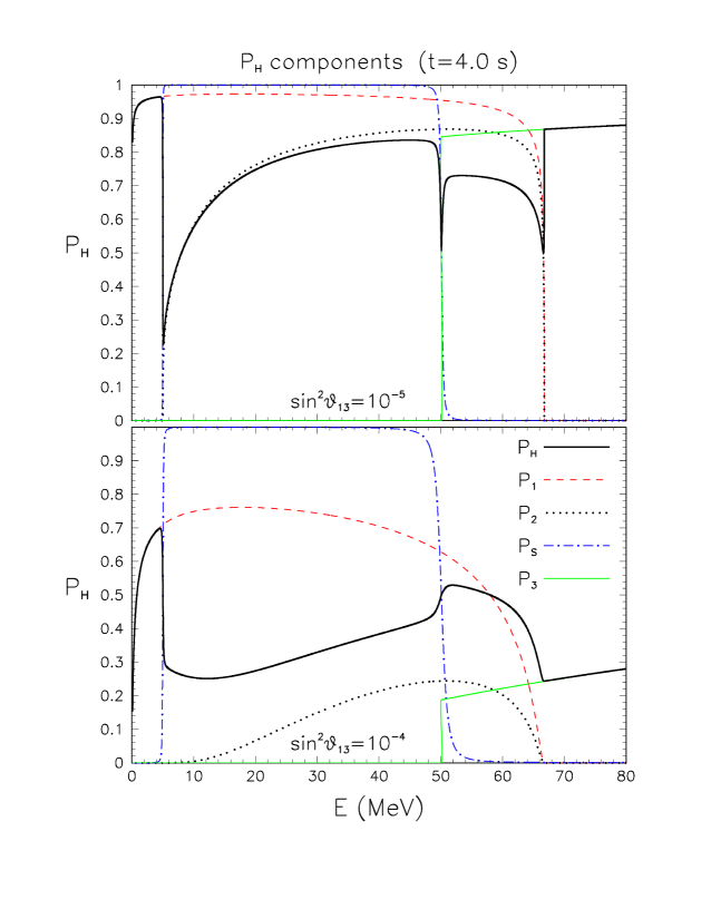
Figure 3: $P_{H}(E)$ in terms of its components $P_{1,2,s,3}$ at $t=4\,\mathrm{s}$, for two representative values of $\sin^{2}\theta_{13}$.

Figure 3 shows the decomposition of $P_{H}(E)$ (analytical, unsmeared) into the four crossing probabilities $P_{1,2,s,3}$ for $\sin^{2}\theta_{13}=10^{-5}$ (top panel) and $\sin^{2}\theta_{13}=10^{-4}$ (bottom panel). In both cases, the shock wave profile at $t=4$ s (see Fig. 1) is assumed. The various transition probabilities are switched on and off at the three critical energies ($E\simeq 5$, 50, and 67 MeV) associated to such profile, as previously discussed.

In the top panel of Fig. 3, both $P_{1}$ and $P_{3}$ are strongly nonadiabatic ($\sim\!1$), and thus $P_{H}=P_{1}\sim 1$ and $P_{H}=P_{3}\sim 1$ in the single-transition regimes at low and high energy, respectively. At intermediate energies both $P_{s}$ and $P_{2}$ are nonzero, but the nonadiabatic character of $P_{2}$ is less pronounced, since at $x_{2}$ (outer part of the rarefaction zone), the density gradient is smaller [and the scale factor in Eq. (16) is larger] than at $x_{1}$ or $x_{3}$—at least in our simplified description of the density profile. Therefore, in the intermediate regime $5\stackrel{{\scriptstyle\textstyle<}}{{\raisebox{-2.58334pt}{$\sim$}}}E\stackrel{{\scriptstyle\textstyle<}}{{\raisebox{-2.58334pt}{$\sim$}}}50$ MeV, the strong nonadiabaticity of $P_{1}$ and $P_{s}$ implies $P_{H}\sim P_{2}$ through Eq. (25). In summary, in the top panel of Fig. 3, the overall crossing probability $P_{H}$ initially takes the value $P_{1}$, then $P_{2}$, and eventually $P_{3}$, as the energy increases and passes through its critical values. All relevant parts of the density profile (static profile, shock front, and both sides of the rarefaction zone) can thus contribute to the $P_{H}$ energy profile.

In the bottom panel of Fig. 3, the higher value of $\sin^{2}\theta_{13}$ leads to an overall decrease of $P_{1,2,3}$, particularly for the second transition ($P_{2}\sim 0$), while $P_{s}$ remains strongly nonadiabatic. Therefore, the behavior of $P_{H}$ is not obvious, except at very low energy (where only $P_{1}>0$) or at very high energy (where only $P_{3}>0$). We can only say that the smallness of $P_{2}$ implies that the outer part of the rarefaction zone (just behind the shock front) are not relevant in this case.

Summarizing, variations of $\sin^{2}\theta_{13}$ for fixed density profile can modulate significantly the $P_{1,2,3}$ contributions to the crossing probability $P_{H}$. The contribution of $P_{s}$ remains instead stable and strongly nonadiabatic. As a consequence, different parts of the neutrino profile can play leading or subleading roles, according to the chosen value of $\theta_{13}$. When $\theta_{13}$ will be known, one shall be able to gauge the relative importance of such contributions, and to determine which parts of the shock profile should be most intensively studied. In the meantime, all parts of the shock profile should be considered as potentially important and worth further study.

IV.3 $P_{H}(E)$ at different times, and comments on $P_{L}$

We conclude the analysis in the energy domain by briefly discussing the variations of $P_{H}(E)$ for different post-bounce times $t$. We also comment on the contribution of the shock-front discontinuity to $P_{L}$.

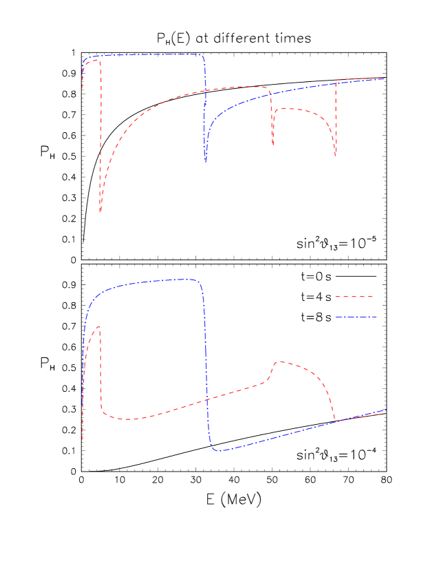
Figure 4: $P_{H}(E)$ at $t=0$, 4, and $8\,\mathrm{s}$, for two representative values of $\sin^{2}\theta_{13}$.

Figure 4 shows the function $P_{H}(E)$ at three different times ($t=0$, 4, and 8 s) for $\sin^{2}\theta_{13}=10^{-5}$ (top panel) and $10^{-4}$ (bottom panel). The curves at $t=4\,\mathrm{s}$ have already been discussed. At earlier times $t\stackrel{{\scriptstyle\textstyle<}}{{\raisebox{-2.58334pt}{$\sim$}}}1\,\mathrm{s}$ ($t=0\,\mathrm{s}$ in Fig. 4) the behavior of $P_{H}$ becomes simpler, being basically dictated by a single LZ crossing along the static profile. At later times $(t=8\,\mathrm{s})$, the critical energies at which $k_{H}=V^{\pm}$ and $k_{H}=V(x_{r})$ move forward and partly fall outside the energy range relevant for supernova neutrinos. As a consequence, the nonadiabatic character of the innermost transition at $x_{1}$ makes $P_{H}\sim 1$ in almost the first half of the energy range of Fig. 4, with a rapid drop to smaller values as the more adiabatic transition $P_{2}$ becomes relevant. The drift of the zones where $P_{H}$ is high or low has thus an interesting time structure, which is analyzed in more detail in the next section.

We conclude this section with a few comments on the crossing probability $P_{L}$ in the $L$ subsystem. As mentioned in Sec. II C, the step-like nature of the shock front profile can make $P_{L}\simeq P_{s}\neq 0$ for $k_{L}$ roughly within the range $[V^{-},V^{+}]$. In practice, however, this condition occurs only in the low-energy tail of the (anti)neutrino spectrum $(E\stackrel{{\scriptstyle\textstyle<}}{{\raisebox{-2.58334pt}{$\sim$}}}\mathrm{few\ MeV})$ and at relatively late times $(t\stackrel{{\scriptstyle\textstyle>}}{{\raisebox{-2.58334pt}{$\sim$}}}10\,\mathrm{s})$. Low-energy effects are suppressed by the lower cross section and by experimental detection thresholds, while late-time effects are intrinsically suppressed by the exponential decrease of the supernova neutrino luminosity on a timescale of a few seconds (see also Sec. VI). Moreover, the $L$-transition is never strongly nonadiabatic; in fact, from Eq. (19) one can prove that $P_{L}(\nu)$ and $P_{L}(\overline{\nu})$ are always significantly smaller than $\cos^{2}\theta_{12}$ and $\sin^{2}\theta_{12}$, respectively. For such reasons, effects related to $P_{L}\neq 0$ at the shock front are hardly observable, and have been neglected throughout this work.

V Analysis of crossing probabilities in the time domain

In this Section we study in detail the time dependence of $P_{H}$ at fixed energy. As in Sec. IV, we start with a comparison between numerical and analytical calculations of $P_{H}$, and then we study the decomposition of $P_{H}$ in terms of $P_{1,2,s,3}$.

V.1 Analytical vs numerical calculations of $P_{H}(t)$

Figure 5 shows our calculation of $P_{H}(t)$ at fixed neutrino energy $E=30$ MeV and for five representative values of $\sin^{2}\theta_{13}$, ranging from $10^{-6}$ (top) to $10^{-2}$ (bottom). In the left panels, a direct comparison is made between analytical calculations (solid curves) and Runge-Kutta numerical calculations (dots), performed at $5\times 10^{3}$ equally-spaced points in the shown time interval. Once again, the interference among multiple $\nu$ transition amplitudes appears to generate fast oscillations, which scatter the numerical results around the analytical curves. In the right panels of Fig. 5, phase averaging (smearing) is instead enforced through a convolution with a “top-hat” time resolution function with $\pm 0.5\,\mathrm{s}$ width. It can be seen that such phase averaging brings the numerical and analytical calculations in very good agreement at any $t$, up to small residual artifacts in the smeared numerical results, which would disappear by sampling the abscissa more densely (not shown). From the results of Figs. 2 and 5 we conclude that simple, analytical calculations provide the correct phase-averaged value of $P_{H}$ as a function of both $E$ and $t$. Therefore, time-consuming numerical estimates of neutrino transitions along the shock profile Schi ; Shoc can be accurately replaced by much faster and elementary calculations. This is one of the main results of our work.

Let us now discuss in more detail the behavior of the analytical $P_{H}$ in the left panels of Fig. 5. In analogy with the previous discussion in the energy domain, the structure of $P_{H}$ appears to be characterized by (up to) four different regimes also in the time domain. These regimes are separated by three “critical times,” namely, $t\simeq 3.2\,\mathrm{s}$ (when $k_{H}$ equals $V$ at the bottom of the rarefaction zone $x_{r}$), $t\simeq 3.3\,\mathrm{s}$ (when $k_{H}$ equals $V^{-}$ at the bottom of the shock front), and $t\simeq 7.7\,\mathrm{s}$ (when $k_{H}$ equals $V^{+}$ at the top of the shock front). [Of course, for $E\neq 30$ MeV such critical times will be different.] The probabilities $P_{1,2,s,3}$ play different roles in forming the global $P_{H}(t)$ in these different regimes. For $t\stackrel{{\scriptstyle\textstyle<}}{{\raisebox{-2.58334pt}{$\sim$}}}3.2$ s, the relevant density profile is essentially static, and $P_{H}\simeq P_{3}\propto\mathrm{const}^{\sin^{2}\theta_{13}}$. Similarly, for $t\stackrel{{\scriptstyle\textstyle>}}{{\raisebox{-2.58334pt}{$\sim$}}}7.7\,\mathrm{s}$, it is $P_{H}\simeq P_{1}\propto\mathrm{const}^{\sin^{2}\theta_{13}}$. The single-transition values of $P_{H}$ at early and late times are thus reduced by successive powers of ten as $\sin^{2}\theta_{13}$ is reduced by factors of ten from top to bottom in Fig. 5. At intermediate times the situation is instead less obvious. For $t\simeq 3.2$–3.3 s, the crossing probabilities $P_{2}$ and $P_{s}$ are switched on in succession, leading to a complex local structure in $P_{H}(t)$ (especially at small $\sin^{2}\theta_{13}$); in this situation, neutrino matter effects are probing the lower part of both the rarefaction zone and of the shock front (see Fig. 1). In the interval $3.3\stackrel{{\scriptstyle\textstyle<}}{{\raisebox{-2.58334pt}{$\sim$}}}t\stackrel{{\scriptstyle\textstyle<}}{{\raisebox{-2.58334pt}{$\sim$}}}7.7$ s, $P_{s}$ is always strongly nonadiabatic, $P_{3}$ is negligible, while $P_{1,2}$ play a role only at small $\sin^{2}\theta_{13}$ (being exponentially suppressed for increasing $\theta_{13}$). For $\sin^{2}\theta_{13}=10^{-2}$ (bottom panels), only $P_{s}$ is important in forming the global $P_{H}$.

The most complicated cases in Fig. 5 thus emerge at “intermediate times” (i.e., when both the rarefaction zone and the shock front are being probed) and at “intermediate $\theta_{13}$ mixing” (i.e., when $P_{1,2,3}$ are moderately nonadiabatic). In such cases, a decomposition of $P_{H}$ into $P_{1,2,s,3}$ is necessary to grasp the main features of $P_{H}(t)$.

V.2 $P_{H}(t)$ decomposition

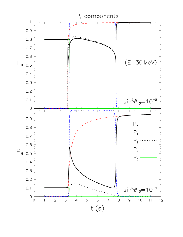
Figure 6: $P_{H}(t)$ in terms of its components $P_{1,2,s,3}$ at $E=30$ MeV, for two representative values of $\sin^{2}\theta_{13}$.

Figure 6 shows the decomposition of $P_{H}(t)$ (analytical, unsmeared) into the four crossing probabilities $P_{1,2,s,3}$ at $E=30$ MeV, for $\sin^{2}\theta_{13}=10^{-5}$ (top panel) and $\sin^{2}\theta_{13}=10^{-4}$ (bottom panel). The various transition probabilities are switched on and off at the three critical times $t\simeq 3.2$, 3.3, and 7.7 s. In both panels, $P_{3}$ and $P_{1}$ dominate at early and late times, respectively. At intermediate times, the structure of $P_{H}$ depends sensitively [through Eq. (25)] upon the specific values of the crossing probabilities $(P_{1,2})$ in the rarefaction zone ($P_{s}$ being almost constant and close to $1$). The results in this figure confirm that variations of $\theta_{13}$ can lead to dramatic variations in the role of each $P_{i}$ (and thus of the different parts of the shock profile) in building the final crossing probability $P_{H}$ as a function of both energy and time.

VI Impact on observable positron spectra

As an application of the analytical calculation of $P_{H}$ described in the previous section, we study the effect of the shock propagation on the energy (and time) spectra of positrons detectable at the Earth through the inverse beta-decay reaction

$$\overline{\nu}_{e}+p\to n+e^{+}\ .$$ (34)

We assume a “standard” supernova explosion at $D=10$ kpc, releasing a total energy $E_{B}=3\times 10^{53}$ erg, equally shared among the (anti)neutrino flavors $\nu_{\alpha}$, and distributed in time as

$$L(t)=\frac{E_{B}}{6\tau}\,e^{-t/\tau}\ ,$$ (35)

where $L$ is the luminosity for each $\nu_{\alpha}$ flux, and the decay time is taken as $\tau=3\,\mathrm{s}$ Schi . For the sake of simplicity, we assume unpinched (normalized) Fermi-Dirac $\nu_{\alpha}$ spectra with time-independent temperatures $T_{\alpha}$,

$$f_{\alpha}(E)=\frac{0.176}{T^{4}_{\alpha}}\,\frac{L(t)}{4\pi D^{2}}\frac{E^{2}}{e^{E/T_{\alpha}}+1}\ ,$$ (36)

where we take $T_{\overline{e}}=4.5$ MeV and $T_{\overline{x}}=6.5$ MeV ($x=\mu,\tau$).

In the presence of oscillations, the supernova $\overline{\nu}_{e}$ spectrum is given by

$$f(E)=f_{\overline{e}}(E)P_{ee}+f_{\overline{x}}(E)(1-P_{ee}),$$ (37)

where $P_{ee}$ is taken from Eq. (21) (antineutrino case). The convolution of $f(E)$ with the differential cross section $d\sigma(E,E_{\mathrm{pos}})/dE_{\mathrm{pos}}$ Stru provides the event spectrum $dN/dE_{\mathrm{pos}}$ in terms of the positron energy $E_{\mathrm{pos}}$. We assume perfect energy resolution and zero threshold, in order to show the shock effects in the most favorable conditions. It is understood that such effects will be somewhat degraded in realistic cases, depending on detector details. Finally, just to fix the overall scale, we assume a detector volume corresponding to 32 kton of water. However, for the main purposes of our discussion, the event rate units could be taken as arbitrary in the following figures.

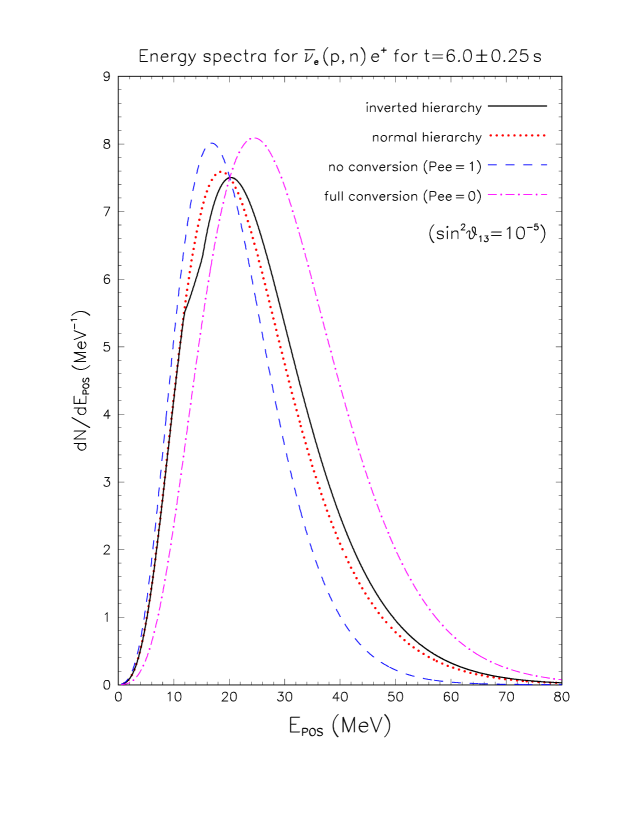
Figure 7: Representative positron energy spectra of supernova antineutrino events from inverse beta decay, for different degrees of $\overline{\nu}_{e}$ conversion into $\overline{\nu}_{x}$. Dashed curve: No conversion. Dot-dashed curve: Full conversion. Dotted line: Partial conversion for normal hierarchy. Solid line: Partial conversion for inverse hierarchy (calculated for $\sin^{2}\theta_{13}=10^{-5}$, and integrated over the time interval $t=6\pm 0.25\,\mathrm{s}$). The latter case shows the shock imprint as a “shoulder” in the spectrum range $E\simeq 10$–20 MeV, .

Figure 7 shows our calculated positron spectra for no oscillations ($P_{ee}=1$, dashed curve) and hypothetical full conversion ($P_{ee}=0$, dot-dashed curve). For partial conversion, Eq. (37) implies that the final positron spectrum is basically a linear combination of the previous two spectra. Examples are given in Fig. 7 for $\sin^{2}\theta_{13}=10^{-5}$, for both normal hierarchy (dotted curve) and inverted hierarchy (solid curve). For normal hierarchy, the coefficients of the combination are energy-independent, namely, $P_{ee}=\cos^{2}\theta_{12}$ and $1-P_{ee}=\sin^{2}\theta_{12}$ [see Eq. 21]. Conversely, for inverse hierarchy, such coefficients become energy- and time-dependent through $P_{H}$ [$P_{ee}=\cos^{2}\theta_{12}P_{H}(E)$]. In the specific example of Fig. 7, the time is fixed through integration over a representative bin [$t=6\pm 0.25\,\mathrm{s}$]. The energy profile of $P_{H}(E)$ then governs the relative weight of the spectra $f_{\overline{e}}$ and $f_{\overline{x}}$ in the combination. As $P_{H}$ decreases from its low-energy value at the first critical energy (see Figs. 3 and 4 and related comments), the weight of $f_{\overline{x}}$ increases and the positron spectrum is shifted to higher energies. The “shoulder” around the peak of the solid curve is thus an imprint of the shock passage. This shoulder is expected to drift for time bins different from $t=6\pm 0.25\,\mathrm{s}$.

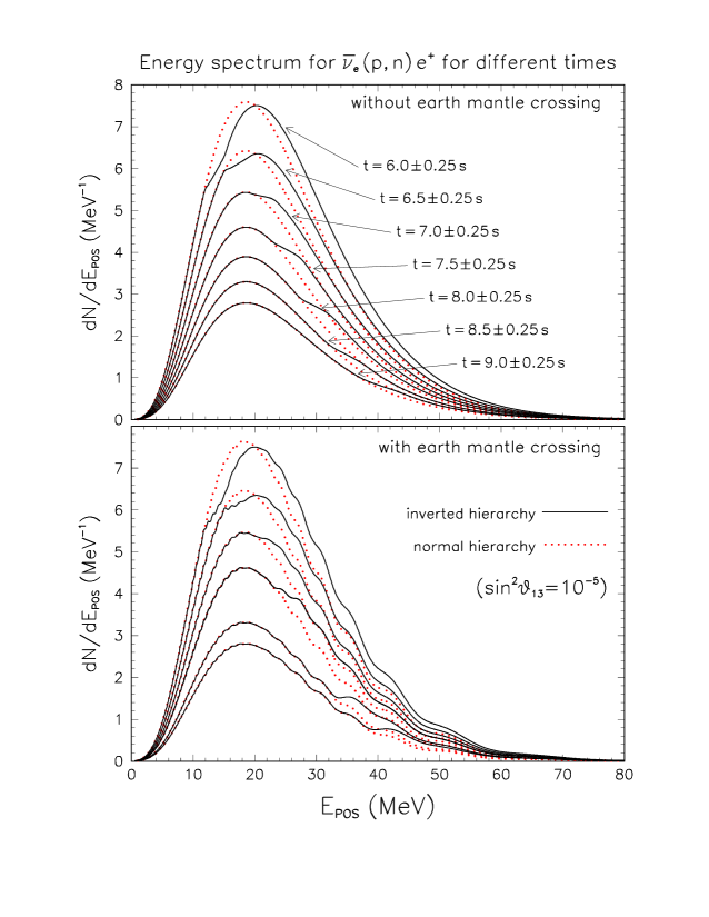
Figure 8: Positron energy spectra for successive time bins, calculated for $\sin^{2}\theta_{13}=10^{-5}$ and for normal and inverted hierarchy (dotted and solid curves, respectively). In the case of inverted hierarchy, shock-induced spectral deformation move forward in energy for increasing post-bounce time. The bottom panel includes representative effects of Earth mantle crossing, which induce additional spectral deformations.

Figure 8 shows a set of successive positron energy spectra, binned in time intervals of 0.5 s, from about 6 to 9 seconds after bounce. The overall decrease of the spectra for increasing $t$ is due to the decrease in luminosity. The top panel does not include Earth effects, while the bottom panels includes representative Earth mantle crossing effects, calculated in the same conditions as in Ours . As in Fig. 7, the cases of normal and inverted hierarchy are distinguished through dotted and solid curves, respectively, and $\sin^{2}\theta_{13}$ is fixed at $10^{-5}$. The top panel shows how the shock passage can leave an observable, time-dependent spectral deformation, in the case of inverse hierarchy. This possibility is very exciting, although one might realistically hope to see no more than variations in the first spectral moments Shoc ; Luna .

From the comparison of the top and bottom panel in Fig. 8, it turns out that the spectral modulation due to the shock might be partly hindered, at late times, by the additional modulation generated by Earth effects. In other words, the “wiggles” produced by oscillations in the Earth might make it difficult to identify the position of the genuine, shock-dependent spectral deformations at different times. Therefore, in some cases Earth effects may not necessarily represent an additional handle Luna to study the shock dynamics via neutrinos.

Finally, Fig. 9 shows the drop in the positron event rate (arbitrary units) as a function of time and for four representative values of $\sin^{2}\theta_{13}$, ranging from $10^{-5}$ to $10^{-2}$. Four rates are displayed in each panel, integrated over consecutive 10 MeV energy bins. For normal hierarchy (dotted curves), the rates decrease according to the assumed exponential law in Eq. (35). For inverted hierarchy (solid curves), the characteristic time structure of $P_{H}(t)$ (see Fig. 5) is instead reflected in a characteristic deviation of the rate decrease with respect to a pure exponential drop: The lower $P_{H}(t)$, the higher the rate (enriched in $\overline{\nu}_{x}$ events) for inverse hierarchy, as compared with normal hierarchy. The two hierarchies become instead indistinguishable when $P_{H}(t)\simeq 1$ (see Fig. 5), since $P_{ee}\simeq\cos^{2}\theta_{12}$ for both normal and inverted neutrino mass spectra [Eq. (21)]. Roughly speaking, the time structure of the event rates in Fig. 9 reflects (although “up-side-down”) the $P_{H}(t)$ pattern in Fig. 5.

Shock-wave signatures in the time domain have been emphasized in Schi . It goes without saying that very high statistics would be needed to discriminate such time structures in real experiments. Nevertheless, the reward could be very high. Let us consider, e.g., the “bathtub” pattern of the solid curves in the lower right panel of Fig. 9 ($\sin^{2}\theta_{13}=10^{-2}$). The (hypothetical) experimental detection of such rather distinctive pattern would, at the same time: ($i$) provide a snapshot (if not a “movie”) of the shock wave propagation; ($ii$) prove that the neutrino mass hierarchy is inverted; and ($iii$) put a significant lower bound on $\sin^{2}\theta_{13}$. Each of these results would have a dramatic impact on our understanding of both supernova and neutrino properties.

VII Summary and prospects

Supernova shock propagation can produce observable effects in the energy and time structure of the neutrino signal, as suggested in Schi and also investigated in Shoc ; Luna . In the calculation of such effects for $3\nu$ oscillations, the neutrino crossing probability $P_{H}$ in the 1-3 neutrino subsystem plays an important role. The evaluation of $P_{H}$ can be done either numerically or analytically, for given shock profiles in space and time. By assuming a simplified description of the time-dependent density profile, we have explicitly shown that simple analytical calculations accurately reproduce the phase-averaged numerical results, also in the nonobvious case of multiple transitions along the shock profile. The analytical approach has then been used to study some relevant characteristics of the structure of $P_{H}$ in energy and time. This structure can in part be reflected in observable signals, as we have shown through some simple and selected examples.

The simplifications used in this work, and especially the empirical parameterization of the density profile, do not alter our main conclusions about the validity and usefulness of a simple analytical approach to $P_{H}$, as compared with brute-force numerical calculations. However, such simplifications may affect the specific values of $P_{H}$ that we have estimated at given energy and time. These values (and the corresponding observable effects) should not be taken too literally, since they depend on features of the shock profile which are beyond our control. In particular, the shape of the rarefaction zone left behind by the shock wave should be constrained, if possible, by dedicated supernova simulations with higher resolution in space and time. When such issues will be clarified, more realistic calculations of $P_{H}$, and of its imprint on observable neutrino signals at the Earth, will become possible.

Figure 5: Comparison of numerical and analytical calculations of the crossing probability $P_{H}(t)$ (dots and solid curves, respectively) at $E=30$ MeV and for five representative values of $\sin^{2}\theta_{13}$. In the right panels, phase effects are time-averaged.

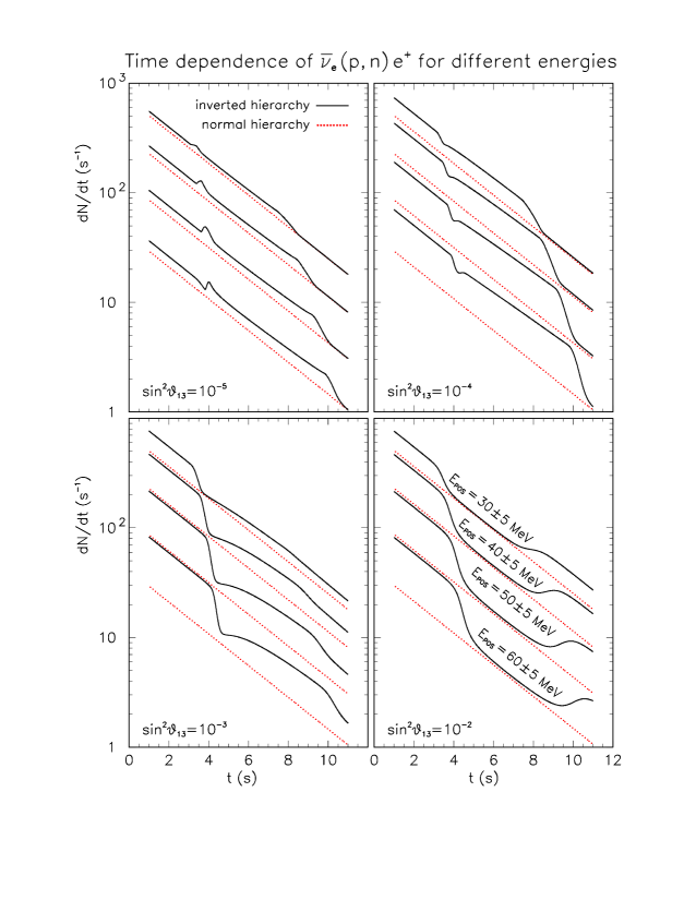
Figure 9: Time dependence of the positron event rate (binned in specified energy intervals) for four representative values of $\sin^{2}\theta_{13}$. For normal hierarchy (dotted lines), the event rate is just proportional to the neutrino luminosity (assumed to decay exponentially in time). For inverted hierarchy (solid lines) an additional time structure is induced by the shock propagation.

- (1) R.C. Schirato and G. M. Fuller, “Connection between supernova shocks, flavor transformation, and the neutrino signal,” astro-ph/0205390.
- (2) Simulations of supernova shock propagation over have been performed by J.R. Wilson and H.E. Dalhed, as quoted in Schi .
- (3) G.G. Raffelt, in the Proceedings of the International School of Physics “Enrico Fermi,” Course 152 (Varenna, Lake Como, Italy, 2002), to appear [hep-ph/0208024].
- (4) J.F. Beacom, in the Proceedings of “Neutrino 2002,” 20th International Conference on Neutrino Physics and Astrophysics (Munich, Germany, 2002), edited by F. von Feilitzsch and N. Schmitz, Nucl. Phys. B (Proc. Suppl.) 118, 307 (2003) [astro-ph/0209136].
- (5) J. Engel, G.C. McLaughlin, and C. Volpe, Phys. Rev. D 67, 013005 (2003) [hep-ph/0209267].
- (6) S. Ando and K. Sato, Phys. Lett. B 559, 113 (2003) [astro-ph/0210502].
- (7) S. Ando and K. Sato, Phys. Rev. D 67, 023004 (2003) [hep-ph/0211053].
- (8) K. Takahashi, K. Sato, H.E. Dalhed, and J.R. Wilson, astro-ph/0212195.
- (9) S. Choubey and K. Kar, hep-ph/0212326.
- (10) C. Lunardini and A.Yu. Smirnov, hep-ph/0302033.
- (11) L. Wolfenstein, Phys. Rev. D 17, 2369 (1978); S.P. Mikheev and A.Yu. Smirnov, Yad. Fiz. 42, 1441 (1985) [Sov. J. Nucl. Phys. 42, 913 (1985)].
- (12) R. Buras, M. Rampp, H.T. Janka, and K. Kifonidis, astro-ph/0303171.
- (13) M.T. Keil, G.G. Raffelt and H.T. Janka, astro-ph/0208035.
- (14) G.G. Raffelt, M.T. Keil, R. Buras, H.T. Janka, and M. Rampp, astro-ph/0303226.
- (15) Particle Data Group Collaboration, K. Hagiwara et al., Phys. Rev. D 66, 010001 (2002).
- (16) G.L. Fogli, E. Lisi, A. Marrone, D. Montanino, A. Palazzo, and A.M. Rotunno, Phys. Rev. D 67, 073002 (2003) [hep-ph/0212127].
- (17) G.L. Fogli, E. Lisi, A. Marrone, and D. Montanino, Phys. Rev. D 67, 093006 (2003) [hep-ph/0303064].
- (18) T.K. Kuo and J. Pantaleone, Rev. Mod. Phys. 61, 937 (1989).
- (19) G.L. Fogli, E. Lisi, D. Montanino, and A. Palazzo, Phys. Rev. D 65, 073008 (2002); (E) 66, 039901 (2002).
- (20) S.T. Petcov, Phys. Lett. B 200, 373 (1988).
- (21) A.S. Dighe and A.Yu. Smirnov, Phys. Rev. D 62, 033007 (2000) [hep-ph/9907423].
- (22) C.S. Lim, K. Ogure, and H. Tsujimoto, Phys. Rev. D 67, 033007 (2003) [hep-ph/0210066].
- (23) A. Strumia and F. Vissani, astro-ph/0302055.