CERN-TH/2003-077

DESY 03-066

ITEP-03-05

The Higgs Sector
of the Next-to-Minimal Supersymmetric Standard Model
D.J. Miller¹, R. Nevzorov²
and P.M. Zerwas^3
1 Theory Division, CERN, CH-1211 Geneva 23, Switzerland
² ITEP, Moscow, Russia
³ Deutsches Elektronen–Synchrotron DESY, D–22603 Hamburg, Germany

The Higgs boson spectrum of the Next-to-Minimal Supersymmetric Standard Model is examined. The model includes a singlet Higgs field $S$ in addition to the two Higgs doublets of the minimal extension. ‘Natural’ values of the parameters of the model are motivated by their renormalization group running and the vacuum stability. The qualitative features of the Higgs boson masses are dependent on how strongly the Peccei-Quinn $U(1)$ symmetry of the model is broken, measured by the self-coupling of the singlet field in the superpotential. We explore the Higgs boson masses and their couplings to gauge bosons for various representative scenarios.

1 Introduction

Supersymmetric models [1, 2] take an important step toward a solution of the hierarchy problem [3] by stabilizing the ratio of the electroweak and Plank/GUT scales. In the Standard Model (SM), the Higgs boson mass gains radiative corrections which depend quadratically on the cut-off scale of the theory (usually taken to be the GUT scale $M_{\rm GUT}\simeq 2\times 10^{16}$ GeV), threatening to generate a mass which is far too large to explain electroweak symmetry breaking. In order to stabilize this mass at a phenomenologically acceptable scale (below a TeV), one must fine tune the parameters of the model, creating an accidental cancellation between the bare mass and the quantum corrections. By introducing a new symmetry, a supersymmetry [1] between bosons and fermions, one introduces new contributions to the quantum corrections to the Higgs mass. The supersymmetry ensures that the contribution of new supersymmetric particles exactly cancel the quadratic divergence of their Standard Model partners, removing the sensitivity of the Higgs mass to the cut-off scale in a natural way.

The Minimal Supersymmetric Standard Model (MSSM) contains a scale $\mu$, the Higgs-higgsino mass parameter in the superpotential, which is phenomenologically constrained to lie not far from the electroweak scale [4]; in the Next-to-Minimal Supersymmetric Standard Model (NMSSM) this mass parameter may be linked dynamically to the electroweak scale in a natural way [5]–[10]. The superpotential of the MSSM must be analytic in the fields, preventing the use of only one Higgs doublet for the generation of both up-type and down-type quark masses. Thus the model requires two Higgs doublets, which is also necessary to maintain an anomaly free theory. One of the doublets ($H_{u}$) provides a mass for up-type quarks while the other ($H_{d}$) provides a mass for down-type quarks and charged leptons. The term $\mu H_{u}H_{d}$ in the superpotential of the MSSM mixes the two Higgs doublets. Since the parameter $\mu$, present before the symmetry is broken, has the dimension of mass, one would naturally expect it to be either zero or the Planck scale ($M_{\rm Pl}$). However, if $\mu=0$ then the form of the renormalization group equations [11] implies that the mixing between Higgs doublets is not generated at any scale; the minimum of the Higgs potential occurs for $\langle H_{d}\rangle=0$, causing the down-type quarks and charged leptons to remain massless after symmetry breaking. In the opposite case, for $\mu\simeq M_{\rm Pl}$, the Higgs scalars acquire a huge contribution $\mu^{2}$ to their squared masses and the fine tuning problem is reintroduced. Indeed, one finds that $\mu$ is required to be of the order of the electroweak scale in order to provide the correct pattern of electroweak symmetry breaking.

The most elegant solution of this $\mu$–problem is to introduce a new singlet Higgs field $S$, and replace the $\mu$-term $\mu H_{u}H_{d}$ by an interaction $\lambda S(H_{u}H_{d})$. When the extra scalar field $S$ acquires a non-zero vacuum expectation value (VEV) an effective $\mu$-term of the required size is automatically generated, and the effective $\mu$ parameter may then naturally be expected to be of the electroweak scale, $\mu=\lambda\langle S\rangle$. In this way $\mu$ can be linked dynamically to the scale of electroweak symmetry breaking (although the mechanism generating the common scale of order $100$ GeV to $1$ TeV is left unexplained). This situation naturally appears in the framework of superstring–inspired $E_{6}$ models [13]. At the string scale, the $E_{6}$ symmetry can be broken, leading to the usual low energy gauge groups with additional $U(1)$ factors (for instance $SO(10)\times U(1)\times\ldots$). These extra $U(1)$ symmetries can be broken via the Higgs mechanism in which the scalar components of chiral supermultiplets acquire non-zero VEVs in such a way that all additional gauge bosons and exotic particles acquire huge masses and decouple, except for one singlet field $S$ and a pair of Higgs doublets $H_{u}$ and $H_{d}$.

However, this model still possesses an extra global $U(1)$ symmetry, a Peccei–Quinn (PQ) symmetry [14], which is explicitly broken in the MSSM by the $\mu$-term itself. The breaking of this extra $U(1)$ at the electroweak scale leads to the appearance of a massless CP–odd scalar in the Higgs boson spectrum, the PQ axion [15]. Unfortunately, this axion leads to astrophysical and cosmological constraints which rule out most of the allowed parameter space, leaving only a small window with $10^{-7}<\lambda<10^{-10}$ [16]. Due to the very small value of $\lambda$, a very large value of $\langle S\rangle$ would be required to generate $\mu$ in the required energy range, and this model is unsatisfactory as a solution to the $\mu$-problem. However, this massless axion may be avoided by introducing a term cubic in the new singlet superfield in the superpotential. This term explicitly breaks the additional $U(1)$ global symmetry, providing a mass to the CP–odd scalar. This model is known as the Next–to–Minimal Supersymmetric Standard Model (NMSSM), and is described by the superpotential

$$W=\hat{u}^{c}\,\mathbf{h_{u}}\hat{Q}\hat{H}_{u}-\hat{d}^{c}\,\mathbf{h_{d}}\hat{Q}\hat{H}_{d}-\hat{e}^{c}\,\mathbf{h_{e}}\hat{L}\hat{H}_{d}+\lambda\hat{S}(\hat{H}_{u}\hat{H}_{d})+\frac{1}{3}\kappa\hat{S}^{3}.$$ (1)

Despite the removal of the PQ symmetry, the NMSSM superpotential is still invariant under a discrete $\mathbb{Z}_{3}$ symmetry: $\Phi\to e^{2\pi i/3}\Phi$, where $\Phi$ denotes the observable superfields. Left untamed, this $\mathbb{Z}_{3}$ symmetry would lead to the formation of domain walls in the early universe between regions which were causally disconnected during the period of electroweak symmetry breaking [17]. Such domain wall structures of the vacuum create unacceptably large anisotropies in the cosmic microwave background [18]. In an attempt to break the $\mathbb{Z}_{3}$ symmetry, operators suppressed by powers of the Planck scale can be introduced. However, it has been shown that these operators, in general, give rise to quadratically divergent tadpole contributions, which once again lead to a destabilization of the mass hierarchy [19]. This problem can be circumvented by introducing new discrete symmetries to forbid or loop suppresses the dangerous tadpole contributions. In this case the breaking of the $\mathbb{Z}_{3}$ symmetry should be small enough to not upset the mass hierarchy but large enough to prevent the problematic domain walls [20, 21]. Indeed, in these scenarios one would expect the surviving tadpole terms to be sufficiently suppressed to not effect the low-energy phenomenology described in this study.

We analyze the mass spectrum of the NMSSM paying attention in this report not only to the lowest mass state but also to the heavier Higgs bosons. Characteristic mass patterns emerge for natural choices of the parameters. An important parameter is the extent to which the PQ symmetry is broken, measured by the size of the dimensionless coupling $\kappa$. Moreover, the couplings of the Higgs bosons to the $Z$ boson are studied for several representative scenarios appropriate to the production of the NMSSM Higgs bosons at the next generation of proton and electron-positron colliders.

A central point of the paper is the analytical analyses of the Higgs mass spectrum and couplings in the approximation where the supersymmetry scale is large and the Higgs parameter $\tan\beta$ is moderate to large. The concise formulae which can be derived in this parameter range describe the system to surprisingly high accuracy while providing a valuable analytical understanding of the NMSSM Higgs sector, which is significantly more complicated than the minimal extension.

The paper is organized as follows. In Sec.(2) we describe the Higgs sector of supersymmetric models with an additional singlet superfield. The vacuum is examined and used to place constraints on the parameter space. The Higgs mass matrices are discussed, and an approximate diagonalization of the CP–even mass matrix is used to provide analytic expressions for the masses and mixings, from which the couplings to the $Z$ boson can be derived. These expressions are used to give a qualitative understanding of how the masses and couplings depend upon the parameters. In Sec.(3) the Higgs boson spectrum of the NMSSM is considered for three representative parameter choices in detail, characterized by the breaking of the PQ symmetry. Natural values for the parameters are motivated and it is shown that the renormalization group flow from the GUT scale down to the electroweak scale prefers scenarios where the PQ symmetry is only slightly broken. In this case, two CP–even Higgs bosons and the lightest CP–odd Higgs boson have masses of order $100$ GeV, while one CP–even, one CP–odd and the charged Higgs bosons are heavy. The couplings of the lightest Higgs bosons to the $Z$ are reduced preventing their detection at LEP if kinematically possible otherwise. However, their observation is possible at a future linear collider operating in the TeV energy range with high luminosity, so that the NMSSM may be distinguished from the MSSM at such a facility. If the PQ symmetry is strongly broken for large values of $\kappa$, the extra fields may become more massive and eventually decouple, making such a comparison more difficult. The results are summarized in the Sec.(4). In the appendix, approximate solutions for the masses and couplings of CP–even Higgs bosons are deduced for physically appealing parameter domains.

2 The NMSSM Higgs Sector

2.1 The NMSSM Higgs Potential

The NMSSM Higgs sector is distinguished from that for the MSSM by the addition of an extra complex scalar field, $S$. The Higgs fields of the model then consist of the usual two Higgs doublets together with this extra Higgs singlet,

$$H_{u}=\left(\begin{array}[]{c}H_{u}^{+}\\ H_{u}^{0}\end{array}\right),\quad H_{d}=\left(\begin{array}[]{c}H_{d}^{0}\\ H_{d}^{-}\end{array}\right),\quad S.$$ (2)

In the superpotential, already presented in Eqn.(1), the extra singlet is allowed to couple only to the Higgs doublets of the model, and consequently the couplings of the new fields to gauge bosons will only be manifest via their mixing with the other Higgs fields. The superpotential leads to the tree–level Higgs potential [9]:

$$V=V_{F}+V_{D}+V_{\rm soft},$$ (3)

with

$$V_{F} = |\lambda S|^{2}(|H_{u}|^{2}+|H_{d}|^{2})+|\lambda H_{u}H_{d}+\kappa S^{2}|^{2},$$ (4)

$$V_{D} = \frac{1}{8}\bar{g}^{2}(|H_{d}|^{2}-|H_{u}|^{2})^{2}+\frac{1}{2}g^{2}|H_{u}^{\dagger}H_{d}|^{2},$$ (5)

$$V_{\rm soft} = m_{H_{u}}^{2}|H_{u}|^{2}+m_{H_{d}}^{2}|H_{d}|^{2}+m_{S}^{2}|S|^{2}+[\lambda A_{\lambda}SH_{u}H_{d}+\frac{1}{3}\kappa A_{\kappa}S^{3}+\textrm{h.c.}],$$ (6)

where $\bar{g}=\sqrt{g^{2}+g^{\prime 2}}$ with $g$ and $g^{\prime}$ being the gauge couplings of $SU(2)_{L}$ and $U(1)$ interactions respectively, and adopting the notation $H_{u}H_{d}\equiv\epsilon_{\alpha\beta}(H_{u})^{\alpha}(H_{d})^{\beta}=H_{u}^{+}H_{d}^{-}-H_{u}^{0}H_{d}^{0}$. The first two terms, $V_{F}$ and $V_{D}$, are the $F$ and $D$ terms derived from the superpotential in the usual way. We also include additional soft supersymmetry breaking terms, $V_{\rm soft}$, by adding all the forms in the superpotential with arbitrary (dimensionful) coefficients, and soft mass terms for the fields. This leads to the inclusion of the extra parameters: $A_{\lambda}$, $A_{\kappa}$, $m_{H_{u}}$, $m_{H_{d}}$ and $m_{S}$.

The parameter combinations $\lambda A_{\lambda}$ and $\kappa A_{\kappa}$ may always be taken to be real and positive since their complex phases may be absorbed into global redefinitions of $H_{u}H_{d}$ and $S$. However, $\lambda$ and $\kappa$ (and therefore $A_{\lambda}$ and $A_{\kappa}$) may be complex. Significantly, if the combination $\lambda\kappa^{*}$ is complex then CP will be violated at tree–level in the Higgs sector. This is in contrast to the MSSM where tree–level CP conservation is guaranteed by the structure of the Higgs potential. In this paper we will adopt the usual convention of assuming that all four parameters are real. For studies of the CP–violating NMSSM see Ref.[22].

While the essential new elements of the Higgs sector can be elaborated at the tree-level, one-loop contributions to the Higgs masses and couplings from top and stop loops are included in the quantitative analyses by introducing the term $V_{\rm loop}$ into the potential, with [23]

$$\langle V_{\rm loop}\rangle=\frac{3}{32\pi^{2}}\left[m_{\tilde{t}_{1}}^{4}\left(\log\frac{m_{\tilde{t}_{1}}^{2}}{Q^{2}}-\frac{3}{2}\right)+m_{\tilde{t}_{2}}^{4}\left(\log\frac{m_{\tilde{t}_{2}}^{2}}{Q^{2}}-\frac{3}{2}\right)-2m_{t}^{4}\left(\log\frac{m_{t}^{2}}{Q^{2}}-\frac{3}{2}\right)\right].$$ (7)

The dependence on the Higgs fields is implicitly contained in the top, $m_{t}$, and stop masses, $m_{\tilde{t}_{1,2}}$, which are dependent, in total or partially, on the Higgs VEVs. For the stop masses, we use the tree–level relation,

$$m^{2}_{\tilde{t}_{2/1}}=\frac{1}{2}\left(m_{Q}^{2}+m_{U}^{2}+2m_{t}^{2}\pm\sqrt{(m_{Q}^{2}-m_{U}^{2})^{2}+4m_{t}^{2}X_{t}^{2}}\right),$$ (8)

where we set $m_{Q}=m_{U}=M_{SUSY}=1$ TeV, the running top quark mass $m_{t}=165$ GeV and, as an example, assume maximal mixing, $X_{t}=\sqrt{6}M_{SUSY}$. The two physical stop masses are given by $m_{\tilde{t}_{1}}=789$ GeV and $m_{\tilde{t}_{2}}=1196$ GeV for these parameters. The renormalization scale, $Q$, is taken to be the running top quark mass. For the present analysis one-loop expressions for the masses and couplings suffice. The explicit expressions for the one-loop corrections to the mass matrices were adopted from Ref.[24].

The “MSSM limit” can be approached smoothly by letting $\lambda$ and $\kappa\to 0$ on a linear trajectory (i.e. $\kappa/\lambda$ constant), while keeping the $\mu$ parameter $\mu=\lambda v_{s}/\sqrt{2}$ and the parameters $A_{\lambda}$ (which plays the role of $B$ in the MSSM) and $A_{\kappa}$ fixed. In this limit the Higgs singlet field decouples from the system completely, and we regain the doublet Higgs sector of the MSSM in its canonical structure.

The structure of the vacuum can be simplified by making a $SU(2)_{L}\times U(1)_{Y}$ gauge transformation to choose $\langle H_{u}^{-}\rangle=0$. In order to ensure that $\langle H_{d}^{-}\rangle=0$ is a suitable choice of vacuum, i.e. that the vacuum is uncharged, one also requires that it be a stable minimum with respect to small perturbations in $H_{d}^{-}$, corresponding to a positive charged Higgs mass-squared:

$$\langle\frac{\partial^{2}V}{\partial H_{d}^{-}\,\partial H_{d}^{-\,*}}\rangle=m_{H_{d}}^{2}+\frac{1}{2}\lambda^{2}|v_{s}|^{2}+\frac{1}{8}g^{2}(|v_{u}|^{2}+|v_{d}|^{2})-\frac{1}{8}g^{\prime 2}(|v_{u}|^{2}-|v_{d}|^{2})>0,$$ (9)

where $v_{u}$ and $v_{d}$ are the VEVs of $H_{u}^{0}$ and $H_{d}^{0}$ respectively, multiplied by a factor of $\sqrt{2}$. The resulting vacuum has been studied in Ref.[9], where it was shown that there are three degenerate vacua which differ in the complex phases of $\langle S\rangle$ and $\langle H_{d}^{0}\rangle$. Here, we will restrict ourselves to a discussion of the vacuum where all the remaining VEVs are real, as described by,

$$\langle H_{d}\rangle=\frac{1}{\sqrt{2}}{v_{d}\choose 0},\qquad\langle H_{u}\rangle=\frac{1}{\sqrt{2}}{0\choose v_{u}},\qquad\langle S\rangle=\frac{1}{\sqrt{2}}v_{s},$$ (10)

with $v_{s}$, $v_{u}$, and $v_{d}$ real and positive.

For this vacuum to be a local minimum, we obtain three relations, linking the three soft mass parameters to the three VEVs of the Higgs fields:

$$m_{H_{d}}^{2} = \frac{1}{8}{\bar{g}}^{2}(v_{u}^{2}-v_{d}^{2})-\frac{1}{2}\lambda^{2}v_{u}^{2}+\frac{1}{2}(\sqrt{2}A_{\lambda}+\kappa v_{s})\lambda v_{s}\frac{v_{u}}{v_{d}}-\frac{1}{2}\lambda^{2}v_{s}^{2},$$ (11)

$$m_{H_{u}}^{2} = \frac{1}{8}{\bar{g}}^{2}(v_{d}^{2}-v_{u}^{2})-\frac{1}{2}\lambda^{2}v_{d}^{2}+\frac{1}{2}(\sqrt{2}A_{\lambda}+\kappa v_{s})\lambda v_{s}\frac{v_{d}}{v_{u}}-\frac{1}{2}\lambda^{2}v_{s}^{2},$$ (12)

$$m_{S}^{2} = -\kappa^{2}v_{s}^{2}-\frac{1}{2}\lambda^{2}v^{2}+\kappa\lambda v_{u}v_{d}+\frac{1}{\sqrt{2}}\lambda A_{\lambda}\frac{v_{u}v_{d}}{v_{s}}-\frac{1}{\sqrt{2}}\kappa A_{\kappa}v_{s};$$ (13)

as usual, we have written $v\equiv\sqrt{v_{u}^{2}+v_{d}^{2}}$. The local stability of this vacuum is ensured by allowing only positive squared masses of the physical fields (i.e. the mass eigenstates), which leads to useful constraints on the parameters of the potential.

Proving this to be a global minimum of the vacuum is beyond the scope of this study. However, we consider all possible neutral CP–even vacuum states and ensure that the physical vacuum is of lower energy:

(i) First of all, it is clear that $\langle H_{u}^{0}\rangle=\langle H_{d}^{0}\rangle=\langle S\rangle=0$ is also a stationary point. It must be ensured that this symmetric minimum is not preferred to the physical vacuum with non-zero fields. This is possible in two ways. For the symmetric vacuum to be a stable minimum requires all of $m_{H_{u}}^{2}$, $m_{H_{d}}^{2}$ and $m_{S}^{2}$ to be positive. Therefore, choosing the parameters such that one of the soft masses is negative, is sufficient. However, while sufficient, this constraint is not necessary. Alternatively, one may check that $\langle V\rangle<0$ for the physical vacuum, making it a lower energy state than the symmetric vacuum for which $\langle V\rangle=0$. This constraint places an upper bound on the parameter $A_{\lambda}$.

(ii) The only other neutral CP-even vacua which could be problematic are those where two of $\langle H_{d}^{0}\rangle$, $\langle H_{u}^{0}\rangle$ and $\langle S\rangle$ are zero and the other non-zero. The requirement that the resulting vacuum energy $\langle V\rangle$ is greater for these points than for the physical vacuum can be fulfilled in the major part of the appropriate parameter space. Vacua where only one of $\langle H_{d}^{0}\rangle$, $\langle H_{u}^{0}\rangle$, $\langle S\rangle$ is zero lead to an over-constrained system, so that these vacua can only be realized for very specific choices of the parameters, and may be safely ignored.

The NMSSM Higgs potential is automatically bounded from below for non-zero $\kappa$. The two terms in $V_{F}$ contain contributions which are quartic in the usual neutral Higgs fields, $H_{u}$, $H_{d}$, and in the new scalar, $S$, and will ensure that the potential is bounded from below.

2.2 The Mass Matrices

From the potential, the Higgs mass matrices and subsequently the mass eigenstates can be derived. After shifting the Higgs fields to the minimum of the potential (given by Eqn.(10)), they are rotated by an angle $\beta$ in order to isolate the zero mass Goldstone states, $G$, which are absorbed by the $W$ and $Z$ bosons to provide their masses.

For the charged fields these redefinitions can be written:

$$\begin{array}[]{rcl}H_{d}^{-}&=&H^{-}\sin\beta-G^{-}\cos\beta,\\ H_{u}^{+}&=&H^{+}\cos\beta+G^{+}\sin\beta,\end{array}$$ (14)

where $G^{-}=G^{+\,*}$ and $H^{-}=H^{+\,*}$. For the imaginary and real field components we have

$$\begin{array}[]{rcl}\Im m\,H_{d}^{0}&=&(P_{1}\sin\beta-G^{0}\cos\beta)/\sqrt{2},\\ \Im m\,H_{u}^{0}&=&(P_{1}\cos\beta+G^{0}\sin\beta)/\sqrt{2},\\ \Im m\,S&=&P_{2}/\sqrt{2},\end{array}$$ (15)

and

$$\begin{array}[]{rcl}\Re e\,H_{d}^{0}&=&(-S_{1}\sin\beta+S_{2}\cos\beta+v_{d})/\sqrt{2},\\ \Re e\,H_{u}^{0}&=&(\phantom{-}S_{1}\cos\beta+S_{2}\sin\beta+v_{u})/\sqrt{2},\\ \Re e\,S&=&(S_{3}+v_{s})/\sqrt{2},\\ \end{array}$$ (16)

respectively. Choosing $\tan\beta=v_{u}/v_{d}$ the zero-mass Goldstone modes decouple, and the resulting potential has terms for the non-zero mass modes given by

$$V_{\rm mass}=M_{H^{\pm}}^{2}H^{+}H^{-}+\frac{1}{2}\,(P_{1}\,\,\,P_{2})\,M_{-}^{2}\left(\begin{array}[]{ll}P_{1}\\ P_{2}\end{array}\right)+\frac{1}{2}\,(S_{1}\,\,\,S_{2}\,\,\,S_{3})\,M_{+}^{2}\left(\begin{array}[]{lll}S_{1}\\ S_{2}\\ S_{3}\end{array}\right).$$ (17)

The charged fields $H^{\pm}$ are already physical mass eigenstates with tree-level masses given by
$(I):$

$$M_{H^{\pm}}^{2}=M_{A}^{2}+M_{W}^{2}-\frac{1}{2}(\lambda v)^{2},$$ (18)

where

$$M_{A}^{2}=\frac{\lambda v_{s}}{\sin 2\beta}\left(\sqrt{2}A_{\lambda}+\kappa v_{s}\right).$$ (19)

In contrast, the pseudoscalar and scalar fields, $P_{i}$ ($i=1,\,2$) and $S_{i}$ ($i=1,\,2,\,3$) respectively, are not yet mass eigenstates. Their mass matrices, $M_{-}^{2}$ and $M_{+}^{2}$, must be further rotated to a diagonal basis corresponding to the physical mass eigenstates. Using the minimization conditions, Eqns.(11–13), the tree–level CP–odd matrix has entries,
$(II):$

$$M_{-\,11}^{2} = M_{A}^{2},$$ (20)

$$M_{-\,12}^{2} = \frac{1}{2}(M_{A}^{2}\sin 2\beta-3\lambda\kappa v_{s}^{2})\cot\beta_{s},$$ (21)

$$M_{-\,22}^{2} = \frac{1}{4}(M_{A}^{2}\sin 2\beta+3\lambda\kappa v_{s}^{2})\cot^{2}\beta_{s}\sin 2\beta-3\kappa v_{s}A_{\kappa}/\sqrt{2}.$$ (22)

while the tree–level CP–even matrix is given by,
$(III):$

$$M_{+\,11}^{2} = M_{A}^{2}+(M_{Z}^{2}-\frac{1}{2}(\lambda v)^{2})\sin^{2}2\beta,$$ (23)

$$M_{+\,12}^{2} = -\frac{1}{2}(M_{Z}^{2}-\frac{1}{2}(\lambda v)^{2})\sin 4\beta,$$ (24)

$$M_{+\,13}^{2} = -\frac{1}{2}(M_{A}^{2}\sin 2\beta+\lambda\kappa v_{s}^{2})\cot\beta_{s}\cos 2\beta,$$ (25)

$$M_{+\,22}^{2} = M_{Z}^{2}\cos^{2}2\beta+\frac{1}{2}(\lambda v)^{2}\sin^{2}2\beta,$$ (26)

$$M_{+\,23}^{2} = \frac{1}{2}(2\lambda^{2}v_{s}^{2}-M_{A}^{2}\sin^{2}2\beta-\lambda\kappa v_{s}^{2}\sin 2\beta)\cot\beta_{s},$$ (27)

$$M_{+\,33}^{2} = \frac{1}{4}M_{A}^{2}\sin^{2}2\beta\cot^{2}\beta_{s}+2\kappa^{2}v_{s}^{2}+\kappa v_{s}A_{\kappa}/\sqrt{2}-\frac{1}{4}\lambda\kappa v^{2}\sin 2\beta,$$ (28)

Besides the the usual notation for $\tan\beta$, we have introduced the auxiliary ratio $\tan\beta_{s}\equiv v_{s}/v$. The mass parameter $M_{A}^{2}$ is defined to be the top–left entry of the CP–odd squared mass matrix, c.f. Eqn.(20), which is positive in the physical parameter ranges analyzed later. It becomes the mass of the heavy pseudoscalar Higgs boson in the “MSSM limit”. Parallel to the MSSM, $M_{A}$ replaces the soft parameter $A_{\lambda}$, and at tree–level is given by Eqn.(19).

Higgs Mass Spectrum

The charged Higgs mass has been noted in Eqn.(18). The condition for stability of the vacuum in the $H_{d}^{-}$ direction, Eqn.(9), is simply equivalent to the positivity of $M^{2}_{H^{\pm}}$.

The above pseudoscalar and scalar mass matrices, Eqns. (20–28), do not lend themselves easily to obtaining analytic expressions for the physical Higgs masses. However, reasonably simple expressions can be found by performing a systematic expansion for large $\tan\beta$ and large $M_{A}$ [on the generic electroweak scale]. This is outlined in detail in the appendix. This approximation works extremely well, even for moderate values of $\tan\beta$, and it may therefore be used to shed light on the behaviour of the Higgs masses as the other parameters are varied.

This approximation may be used to simplify the expressions for the tree-level CP-odd masses, giving,

$$M_{A_{2}}^{2} \approx M_{A}^{2}\,(1+\frac{1}{4}\cot^{2}\beta_{s}\sin^{2}2\beta),$$ (29)

$$M_{A_{1}}^{2} \approx -\frac{3}{\sqrt{2}}\kappa v_{s}A_{\kappa},$$ (30)

while the tree-level physical masses of the CP–even Higgs bosons are, in this approximation,

$$M_{H_{3}}^{2} \approx M_{A}^{2}(1+\frac{1}{4}\cot^{2}\beta_{s}\sin^{2}2\beta),$$ (31)

$$M_{H_{2/1}}^{2} \approx \frac{1}{2}\left\{M_{Z}^{2}+\frac{1}{2}\kappa v_{s}(4\kappa v_{s}+\sqrt{2}A_{\kappa})\right.$$ (32)

$$\quad\quad\left.\pm\sqrt{\left[M_{Z}^{2}-\frac{1}{2}\kappa v_{s}(4\kappa v_{s}+\sqrt{2}A_{\kappa})\right]^{2}+\cot^{2}\beta_{s}\left[2\lambda^{2}v_{s}^{2}-M_{A}^{2}\sin^{2}2\beta\right]^{2}}\right\}.$$

The physical mass eigenstates $A_{i}$ and $H_{i}$ are labelled in ascending order of mass.

The heavy CP-odd Higgs boson, $A_{2}$, is approximately degenerate with the heaviest CP-even Higgs boson, $H_{3}$, and the charged Higgs bosons, cf. Eqn.(18). One of the lighter CP-even tree-level masses will be of the order of $M_{Z}$ while the scale of the other is set by $\sim\kappa v_{s}$ for $\kappa$ and $\lambda$ sufficiently below unity. Finally the lightest pseudoscalar mass grows as $\kappa$, $v_{s}$ and $A_{\kappa}$ are increased, with a negative value for $A_{\kappa}$ being preferred.

Range of Parameters

This above solution also allows limits to be placed on the Higgs potential parameters. First of all, the lightest two scalar Higgs boson masses respect a sum rule:

$$M_{H_{1}}^{2}+M_{H_{2}}^{2}\approx M_{Z}^{2}+\frac{1}{2}\kappa v_{s}(4\kappa v_{s}+\sqrt{2}A_{\kappa}).$$ (33)

The right-hand side, and thus the sum of the two lightest scalars, is independent of the coupling $\lambda$ and $M_{A}^{2}$. As a result of this sum rule, the second lightest scalar Higgs boson mass is maximized as the lightest approaches zero.

Furthermore, the smallest eigenvalue of a matrix is smaller than its smallest diagonal entry and similarly the largest eigenvalue is larger than its largest diagonal entry. Together with the above sum rule, this leads to the mass constraints at tree-level (i.e. modified by radiative corrections in parallel to the MSSM):

$$M_{H_{1}}^{2} \lesssim{\rm min}\{M_{Z}^{2},\frac{1}{2}\kappa v_{s}(4\kappa v_{s}+\sqrt{2}A_{\kappa})\},$$ (34)

$${\rm max}\{M_{Z}^{2},\frac{1}{2}\kappa v_{s}(4\kappa v_{s}+\sqrt{2}A_{\kappa})\}\lesssim M_{H_{2}}^{2} \lesssim M_{Z}^{2}+\frac{1}{2}\kappa v_{s}(4\kappa v_{s}+\sqrt{2}A_{\kappa}).$$ (35)

A further constraint is found by exploiting the condition that the mass-squared of the lightest Higgs boson, given in Eqn.(32), is greater than zero. This in turn gives a restriction on the allowed values of $M_{A}$. At tree–level, again to the accuracy of the approximate solution, this is,

$$M_{A}^{2}\,\lessgtr\,\frac{2\lambda^{2}v_{s}^{2}}{\sin^{2}2\beta}\pm\frac{M_{Z}\tan\beta_{s}}{\sin^{2}2\beta}\sqrt{\frac{\kappa v_{s}}{2}(4\kappa v_{s}+\sqrt{2}A_{\kappa})},$$ (36)

which generalises the corresponding constraint for zero $\kappa$ in Ref. [21]. In the theoretically preferred scenarios where $\kappa$ is small, the second term above is small compared to the first term, and we find that the value of $M_{A}$ is constrained to lie in a narrow bracket, not too far from the value $\sqrt{2}\lambda v_{s}/\sin 2\beta=2\mu/\sin 2\beta$ which is approximately $M_{A}\approx\mu\tan\beta$ for medium to large values of $\tan\beta$. As can be seen from Eqn.(32), this is also the approximate value of $M_{A}$ for which $M_{H_{1}}$ is maximal (and $M_{H_{2}}$ minimal). The constraint on $M_{A}$ becomes stronger as $\kappa$ becomes smaller but $v_{s}$ is kept fixed. The mass parameter $M_{A}$ is not constrained in the proper “MSSM limit” defined earlier with $\lambda v_{s}$ and $\kappa v_{s}$ fixed for $\lambda$ and $\kappa\to 0$.

Finally, one may also gain some insight into the allowed range of the soft SUSY breaking parameter $A_{\kappa}$. Requiring the lightest scalar and pseudoscalar mass-squareds be positive leads to upper and lower constraints on $A_{\kappa}$. At tree–level, these are given by,

$$-2\sqrt{2}\kappa v_{s}\lesssim A_{\kappa}\lesssim 0.$$ (37)

The lower bound is derived from the requirement that the maximum value of the lightest scalar mass-squared be positive, which is realized for the central value of $M_{A}$ given in Eqn.(36). For values of $M_{A}$ deviating from this, the lower bound will become stronger.

One should bear in mind that most of these constraints are based upon the approximate solution as described in the appendix, and will become unreliable in regions of parameter space where the approximate solution breaks down. Nevertheless they provide the proper analytical understanding of the exact numerical results presented in Sec.(3).

2.3 Couplings with the $Z$ boson

The couplings of the Higgs bosons to the $Z$ boson are given by the Lagrangian,

$${\cal L}_{ZAH} = \frac{\bar{g}}{2}M_{Z}Z_{\mu}Z^{\mu}S_{2}+\frac{\bar{g}}{2}Z_{\mu}\left[S_{1}(\partial^{\mu}P_{1})-P_{1}(\partial^{\mu}S_{1})\right]$$ (38)

$$\qquad+\left(eA_{\mu}+\frac{\bar{g}}{2}Z_{\mu}\cos 2\theta_{W}\right)i\left[H^{-}(\partial^{\mu}H^{+})-H^{+}(\partial^{\mu}H^{-})\right],$$

where $Z^{\mu}$ and $A^{\mu}$ are the $Z$ boson and photon fields respectively, $\theta_{W}$ is the weak mixing angle and the Higgs fields have been defined in Eqns.(14–16). The simple form of this Lagrangian arises from the rotation made on the CP–even Higgs states. This leads to $S_{2}$ being the only field with a coupling of the form $ZZS_{i}$, while the scalar and pseudoscalar fields are coupled jointly to $Z$ only in the form $ZS_{1}P_{1}$. The couplings of the extra scalar and pseudoscalar Higgs bosons to the $Z$ are due only to their mixing with the Higgs doublet degrees of freedom. We define this mixing of the CP–odd Higgs bosons via a rotation by an angle $\theta_{A}$ which transforms the fields to their physical mass eigenstates:

$$\left(\begin{array}[]{c}A_{2}\\ A_{1}\end{array}\right)=\left(\begin{array}[]{cc}\cos\theta_{A}&\sin\theta_{A}\\ -\sin\theta_{A}&\cos\theta_{A}\end{array}\right)\left(\begin{array}[]{c}P_{1}\\ P_{2}\end{array}\right).$$ (39)

At tree–level, the mixing angle, $\theta_{A}$, is given by,

$$\tan\theta_{A}=\frac{M_{-\,12}^{2}}{M_{-\,11}^{2}-M_{A_{1}}^{2}}=\frac{1}{2}\cot\beta_{s}\frac{M_{A}^{2}\sin 2\beta-3\lambda\kappa v_{s}^{2}}{M_{A}^{2}-M_{A_{1}}^{2}}.$$ (40)

Similarly, the more complicated scalar mixing is defined via an orthogonal $3\times 3$ rotation matrix $O$ such that,

$$\left(\begin{array}[]{c}H_{3}\\ H_{2}\\ H_{1}\end{array}\right)=O\left(\begin{array}[]{c}S_{1}\\ S_{2}\\ S_{3}\end{array}\right).$$ (41)

Our notation is such that the fields $A_{i}$, $i=1,2$, and $H_{i}$, $i=1,2,3$ are the mass eigenstates of the pseudoscalar and scalar Higgs sectors respectively, with the numerical suffix denoting their mass hierarchy in ascending order (e.g. $A_{1}$ ($H_{1}$) is the lightest pseudoscalar (scalar) Higgs boson). [The ordering of the states $S_{i}$ has been introduced such that $S_{3}$ is the decoupling singlet.]

It is more useful to discuss the couplings of these Higgs bosons to the $Z$ in terms of normalized couplings. To this end, we define the normalized CP–even couplings by dividing out the associated SM coupling and for the $ZA_{i}H_{j}$ couplings we similarly divide by $\bar{g}/2=\sqrt{g^{2}+g^{\prime\,2}}/2$, so that,

$$\mathcal{G}_{ZZH_{i}}\equiv\frac{g^{\rm NMSSM}_{ZZH_{i}}}{g^{\rm SM}_{ZZH}},\qquad\mathcal{G}_{ZA_{i}H_{j}}\equiv\frac{g^{\rm NMSSM}_{ZA_{i}H_{j}}}{\bar{g}/2}.$$ (42)

The couplings may then be written directly in terms of the mixing matrices, in an obvious notation, according to,

$$\mathcal{G}_{ZZH_{i}}=O_{H_{i}S_{2}},$$ (43)

and

$$\mathcal{G}_{ZA_{1}H_{i}}=-O_{H_{i}S_{1}}\sin\theta_{A},\qquad\mathcal{G}_{ZA_{2}H_{i}}=O_{H_{i}S_{1}}\cos\theta_{A}.$$ (44)

For these normalized couplings the orthogonality of the mixing matrices lead to the constraints,

$$\sum_{i}\mathcal{G}^{2}_{ZZH_{i}}=1,\quad\sum_{ij}\mathcal{G}^{2}_{ZA_{i}H_{j}}=1,\quad\sum_{i}\mathcal{G}_{ZZH_{i}}\mathcal{G}_{ZA_{j}H_{i}}=0.$$ (45)

Finally, the couplings of a pseudoscalar and a scalar to a $Z$ boson are not all independent. The ratios of the two pseudoscalar couplings, $A_{1}$ and $A_{2}$, are independent of the scalar $H_{i}$:

$$\frac{\mathcal{G}_{ZA_{1}H_{1}}}{\mathcal{G}_{ZA_{2}H_{1}}}=\frac{\mathcal{G}_{ZA_{1}H_{2}}}{\mathcal{G}_{ZA_{2}H_{2}}}=\frac{\mathcal{G}_{ZA_{1}H_{3}}}{\mathcal{G}_{ZA_{2}H_{3}}}=-\tan\theta_{A}.$$ (46)

In the approximate solution, where $1/M_{A}$ and $1/\tan\beta$ are regarded as small quantities, the orthogonal matrix $O$ is given by Eqn.(LABEL:eq:Uapprox) in the appendix. Inserting this into Eqn.(43), gives approximate expressions for the scalar-$Z$-$Z$ couplings,

$$\mathcal{G}_{ZZH_{1}}\approx-\sin\theta_{H},\qquad\qquad\mathcal{G}_{ZZH_{2}}\approx\cos\theta_{H},$$ (47)

$$\mathcal{G}_{ZZH_{3}}\approx M_{12}^{2}/M_{11}^{2}\approx\frac{1}{2M_{A}^{2}}\left[\frac{1}{2}(\lambda v)^{2}-M_{Z}^{2}\right]\sin 4\beta,$$ (48)

where $\tan\theta_{H}$ is given by (see Eqn.(78)),

$$\tan\theta_{H}\approx\frac{1}{2}\cot\beta_{s}\frac{2\lambda^{2}v_{s}^{2}-M_{A}^{2}\sin^{2}2\beta-\kappa\lambda v_{s}^{2}\sin 2\beta}{M_{Z}^{2}\cos^{2}2\beta+\frac{1}{2}\lambda^{2}v^{2}\sin^{2}2\beta-M_{H_{1}}^{2}}.$$ (49)

Similarly, for the $Z$-pseudoscalar-scalar couplings we have,

$$\mathcal{G}_{ZA_{1}H_{1}} \approx \frac{1}{4M_{A}^{2}}\left[M_{A}^{2}\sin 2\beta+\kappa\lambda v_{s}^{2}\right]\cot\beta_{s}\cos 2\beta\sin\theta_{A},$$ (50)

$$\mathcal{G}_{ZA_{1}H_{2}} \approx -\frac{1}{2M_{A}^{2}}\left[\frac{1}{2}(\lambda v)^{2}-M_{Z}^{2}\right]\sin 4\beta\sin\theta_{A},$$ (51)

$$\mathcal{G}_{ZA_{1}H_{3}} \approx -\left[1+\frac{1}{4M_{A}^{2}}\left[M_{A}^{2}\sin 2\beta+\kappa\lambda v_{s}^{2}\right]\cot\beta_{s}\cos 2\beta\right]\sin\theta_{A},$$ (52)

and, following from the relations Eqn.(46),

$$\mathcal{G}_{ZA_{2}H_{1}} \approx -\frac{1}{4M_{A}^{2}}\left[M_{A}^{2}\sin 2\beta+\kappa\lambda v_{s}^{2}\right]\cot\beta_{s}\cos 2\beta\cos\theta_{A},$$ (53)

$$\mathcal{G}_{ZA_{2}H_{2}} \approx \frac{1}{2M_{A}^{2}}\left[\frac{1}{2}(\lambda v)^{2}-M_{Z}^{2}\right]\sin 4\beta\cos\theta_{A},$$ (54)

$$\mathcal{G}_{ZA_{2}H_{3}} \approx \left[1+\frac{1}{4M_{A}^{2}}\left[M_{A}^{2}\sin 2\beta+\kappa\lambda v_{s}^{2}\right]\cot\beta_{s}\cos 2\beta\right]\cos\theta_{A},$$ (55)

where $\tan\theta_{A}$ is given by Eqn.(40).

3 NMSSM Higgs boson scenarios

3.1 The parameters

At tree–level the NMSSM Higgs sector described above has six free parameters (apart from the overall scale, set later by the $Z$ boson mass). The Higgs potential, Eqns.(3–6), contained seven parameters: $\lambda$ and $\kappa$ from the superpotential and $A_{\lambda}$, $A_{\kappa}$, $m_{H_{d}}$, $m_{H_{u}}$ and $m_{S}$ from the soft supersymmetry breaking terms. The field values at the minimum of the potential, $v_{u}$, $v_{d}$ and $v_{s}$, are fixed by these parameters according to Eqns.(11–13). The structure of electroweak symmetry breaking allows us to remove one (combination) of these VEVs in favour of the known electroweak scale $v\equiv\sqrt{v_{u}^{2}+v_{d}^{2}}=246$ GeV (or equivalently, the $Z$ boson mass, $M_{Z}$), defining the overall mass scale. Finally, after introducing $\tan\beta\equiv v_{u}/v_{d}$ and writing $A_{\lambda}$ in terms of the heavy Higgs mass scale $M_{A}$, we are therefore left with the six free parameters, $\lambda$, $\kappa$, $v_{s}$, $\tan\beta$, $M_{A}$, and $A_{\kappa}$ ($v_{s}$ may be expressed in some places in terms of the effective $\mu$ parameter, $v_{s}=\sqrt{2}\mu/\lambda$). The spectrum of the NMSSM is expected to show a strong dependence on these six free parameters, which we shall now analyze in detail.

Including higher orders introduces extra parameters such as the top and stop (s)quark masses. We choose to fix these extra parameters at reasonable values and not vary them.

$\lambda$ and $\kappa$

Requiring a weak coupling of the fundamental fields, i.e. field-theoretic perturbativity, in the entire range between the electroweak and GUT scales restricts the range of values for the couplings $\lambda$ and $\kappa$ at the electroweak scale. The renormalization group equations for $\lambda$, $\kappa$ and the top Yukawa coupling $h_{t}$ form a closed set together with those of the gauge couplings. They are given by [6, 11, 25]

$$16\pi^{2}\,\frac{dg_{i}^{2}}{dt} = b_{i}g_{i}^{2},$$ (56)

$$16\pi^{2}\,\frac{dh_{t}^{2}}{dt} = h_{t}^{2}\left[\lambda^{2}+6h_{t}^{2}-\frac{16}{3}g_{3}^{2}-3g_{2}^{2}-\frac{13}{15}g_{1}^{2}\right],$$ (57)

$$16\pi^{2}\,\frac{d\lambda^{2}}{dt} = \lambda^{2}\left[4\lambda^{2}+2\kappa^{2}+3h_{t}^{2}-3g_{2}^{2}-\frac{3}{5}g_{1}^{2}\right],$$ (58)

$$16\pi^{2}\,\frac{d\kappa^{2}}{dt} = 6\kappa^{2}\left[\lambda^{2}+\kappa^{2}\right],$$ (59)

where $b_{1}=33/5$, $b_{2}=1$, $g_{1}=\sqrt{5/3}\,g^{\prime}$, $g_{2}=g$ and $t=\log(Q^{2}/M_{\rm GUT}^{2})$.

Figure 1: The dependence of $\lambda$ (left) and $\kappa$ (right) on renormalization scale, $Q$, for the top Yukawa coupling $h_{t}(M_{\rm GUT})=0.8$. The different curves represent different values of $\lambda$ and $\kappa$ at the GUT scale; left: $\lambda=1$, $2$ and $3$, with $\kappa=1$; right: $\kappa=1$, $2$ and $3$, with $\lambda=1$.

Large values of $\lambda$ and/or $\kappa$ at the GUT scale are greatly reduced when run down to the electroweak scale. This behaviour is caused by the dependence on $\lambda^{4}$ and $\kappa^{4}$ on the right-hand side of Eqns.(58–59) respectively, indicating that large values of these parameters will evolve strongly, while small values evolve only slightly. This can be seen in Fig.(1), which shows the dependence of $\lambda$ and $\kappa$ on renormalization scale. Values of $\lambda$ and $\kappa$ in the perturbative regime at the GUT scale, i.e. $\lambda$, $\kappa\lesssim 2\pi$, are uniformly reduced to small values at the electroweak scale, which may be combined to give the approximate bound, c.f. Fig.(2/left),

$$\lambda^{2}+\kappa^{2}\lesssim 0.5.$$ (60)

Also notice the factor of $6$ in Eqn.(59), compared to the smaller factors in Eqn.(58). This tends to make $\kappa$ run more steeply than $\lambda$, which is further exacerbated by the lack of gauge couplings on the right-hand side of Eqn.(59), since the $\kappa$ term in the superpotential contains only the superfield $\hat{S}$ which has no gauge couplings.

In order to illustrate these behaviours more clearly, we considered $2\times 10^{5}$ different parameter scenarios with (positive) GUT scale values of $\lambda$, $\kappa$ and $h_{t}$ chosen randomly (and independently) between $0$ and $2\pi$, corresponding to the perturbative regime defined by $\kappa/2\pi\lesssim 1$, $\lambda/2\pi\lesssim 1$. Using the renormalization group equations, Eqns.(56–59), to run $\lambda$ and $\kappa$ down to the electroweak scale, the final distribution in $\lambda$ and $\kappa$ can be seen in Fig.(2/right),

Figure 2: Left: The dependence of $\sqrt{\lambda^{2}+\kappa^{2}}$ on renormalization scale, $Q$, for the top Yukawa coupling $h_{t}(M_{\rm GUT})=0.8$. The different curves represent different values of $\lambda$ and $\kappa$ at the GUT scale: $\lambda=\kappa=1$, $2$, and $3$. Right: The electroweak scale values of $\kappa$ and $\lambda$ for $2\times 10^{5}$ different scenarios with random GUT scale values of $0<(\lambda,\kappa,h_{t})<2\pi$. Only scenarios where the running top quark mass $m_{t}(Q)$ falls in the bracket $165\pm 5$ GeV at the electroweak scale are retained. Each point represents a different GUT scale parameter choice.

where each point is a different parameter choice at the GUT scale. Only scenarios where the running top quark mass $m_{t}(Q)$ falls in the bracket $165\pm 5$ GeV at the electroweak scale are retained (approx. $6\%$). This plot demonstrates the limit on $\lambda^{2}+\kappa^{2}$ of Eqn.(60) since no parameter point strays above $\lambda^{2}+\kappa^{2}\approx 0.6$. Furthermore, one can easily see that most of the parameter points lie at low $\kappa$. Nevertheless, the entire area within $\lambda^{2}+\kappa^{2}\lesssim 0.6$ is valuable; the accumulation at the boundary results from the mapping of $\kappa$ and $\lambda$ from the large number of moderately high values at the GUT scale, to small values at the electroweak scale. If $\kappa$ is small at the GUT scale then its renormalization group running will be weak and it will remain small at the electroweak scale.

The size of $\kappa$ governs how strongly the U(1) PQ symmetry of the model is broken. From the above investigation, it is natural to expect that small values of $\kappa$ are preferred and this symmetry is only ‘slightly’ broken. However, this is not a strict bound; scenarios with $\kappa\sim 0.6$ can still occur.

However, if one wants the NMSSM to be a solution to the $\mu$-problem, $\lambda$ must not become too small. We have introduced $v_{s}$ as the VEV of a new Higgs field in order to link $\mu$ to the electroweak (or supersymmetry) scale. If $\lambda$ becomes too small then the phenomenological constraints on $\mu$ require $v_{s}$ to be large and the link with the other Higgs VEVs is lost. Even if we allow $v_{s}$ as large as $3$ TeV (which is a natural upper bound for a weak scale) we would be forced to maintain $\lambda\gtrsim 0.04$. Consequently the allowed values of $\lambda$ are rather constrained.

Even more stringent correlations among the parameters are imposed by grand unified scenarios of the NMSSM including universal boundary conditions for the soft masses and the trilinear couplings. Radiative electroweak symmetry breaking requires the couplings, at the unification scale, $\kappa^{2}$ to be less than about $\lambda^{2}$, and both less than about $0.1$ [7]. To prevent QED and color breaking vacua, the ratio of the universal trilinear coupling and the scalar mass parameter is restricted to values close to $3$ [8]. If universal boundary conditions are not imposed, these constraints will not be effective, of course.

$v_{s}$ and $\tan\beta$

The Higgs-higgsino mass parameter $\mu$ is generally assumed to be in the range $\sim 10^{2}$–$10^{3}$ GeV. However, the ‘natural’ scale for the heavy Higgs masses $M_{A}$ is seen by Eqn.(36) to be of the order of $\mu\tan\beta$. Indeed, this is approximately the value of $M_{A}$ required for the lightest scalar to reach its maximum mass. In order to prevent the mass splitting between the light and heavy Higgs bosons from becoming too large, the value of $\tan\beta$ should be kept moderate, $\lesssim 10$. The value of $v_{s}$ could naturally be expected to vary from $3\,v$ to $15\,v$.

A similar analysis of the renormalization group equations for the other parameters shows that a low value of $\tan\beta$ is favoured [26]. Note that the bounds on $\tan\beta$ derived from the LEP experiments cannot be applied here since these experiments assume MSSM couplings. Referring to the literature for the large $\tan\beta$ case [27], here we will adopt a value of $\tan\beta=3$.

$A_{\kappa}$ and $M_{A}$

The value of $A_{\kappa}$ is tightly constrained by the requirement for vacuum stability, as described in Sec.(2.2). Note that it occurs in only one term of each of the CP–even and CP–odd mass matrices, Eqns.(28, 22), where the two contributions have opposite sign. If $A_{\kappa}$ becomes too large and positive, it will pull the mass–squared of the lightest pseudoscalar below zero, destabilizing the vacuum. On the other hand, if it becomes too large and negative it will destabilize the vacuum by pulling the mass-squared of the lightest scalar negative. This has been quantified in Eqn.(37) and can be seen in Fig.(3)

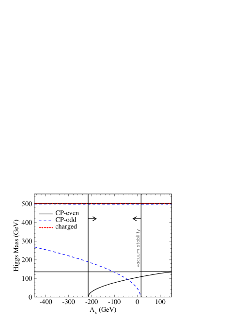
Figure 3: The one-loop Higgs boson masses as a function of $A_{\kappa}$ for $\lambda=0.3$, $\kappa=0.1$, $v_{s}=3\,v$, $\tan\beta=3$ and $M_{A}=\mu\tan\beta\approx 470$ GeV. The arrows denote the physically allowed region.

where the Higgs masses are plotted as a function of $A_{\kappa}$ for reasonable values of the other parameters, including radiative corrections. The heavy Higgs bosons and one of the lighter scalars are very insensitive to the choice of $A_{\kappa}$, but the predominantly singlet scalar and pseudoscalar Higgs bosons exhibit a strong dependence. This is naturally explained by noting that the soft SUSY breaking term containing $A_{\kappa}$ is a cubic coupling proportional to $S^{3}$, so the affect of varying $A_{\kappa}$ is only communicated through the singlet contribution of the Higgs fields. Since the mixing is small, this only affects the two fields which are still singlet dominated.

In contrast to the MSSM, $M_{A}$ is also constrained by vacuum stability in the NMSSM, and, as discussed above and visualized in later plots, its “natural” value is approximately $\mu\tan\beta$. Nevertheless, we will allow $M_{A}$ to vary over the small bracket of its allowed range, including the “natural” value, and plot the Higgs masses as a function of $M_{A}$.

3.2 The NMSSM with the Peccei–Quinn U(1) Symmetry

For illustrative purposes, first consider the simplified case where the U(1) PQ symmetry is left unbroken in the superpotential, achieved by setting $\kappa=0$. The U(1) symmetry is then spontaneously broken by the vacuum, giving rise to a massless Goldstone boson, the PQ axion, which is manifest as the extra pseudoscalar Higgs field. Since there is no SUSY breaking term proportional to $A_{\kappa}$, there are only 4 parameters in the model at tree–level: $\lambda$, $v_{s}$, $\tan\beta$ and $M_{A}$.

While the charged Higgs boson masses are, as usual, given by
$(I):$

$$M_{H^{\pm}}^{2}=M_{A}^{2}+M_{W}^{2}-\frac{1}{2}(\lambda v)^{2},$$ (61)

the tree-level pseudoscalar Higgs boson masses read,
$(II):$

$$M_{A_{2}}^{2} = M_{A}^{2}\,(1+\frac{1}{4}\cot^{2}\beta_{s}\sin^{2}2\beta),$$ (62)

$$M_{A_{1}}^{2} = 0,$$ (63)

where the expressions are exact, with no need of approximation.

The approximate solution, where $1/M_{A}$ and $1/\tan\beta$ are regarded as small parameters of O($\varepsilon$), may again be used to shed light onto the behaviour of the CP–even masses as the parameters are varied. However, due to accidental cancellations, the approximate solution taken to the same order as Eqn.(32), O($\varepsilon^{2}$), always yields a lightest scalar mass-squared that is less than zero. To circumvent this, one must improve the approximate solution to order O($\varepsilon^{4}$). For the scalar Higgs masses, we find
$(III):$

$$\phantom{I):}M_{H_{3}}^{2} \approx M_{A}^{2}\,(1+\frac{1}{4}\cot^{2}\beta_{s}\cos^{2}2\beta\sin^{2}2\beta)+(M_{Z}^{2}-\lambda^{2}v^{2})\sin^{2}2\beta,$$ (64)

$$M_{H_{2}}^{2} \approx \frac{1}{2}\left[M_{Z}^{2}+\sqrt{M_{Z}^{4}+\cot^{2}\beta_{s}\left[2\lambda^{2}v_{s}^{2}-M_{A}^{2}\sin^{2}2\beta\right]^{2}}\right]-(M_{Z}^{2}-\frac{1}{2}\lambda^{2}v^{2})\sin^{2}2\beta,$$ (65)

$$M_{H_{1}}^{2} \approx \frac{1}{2}\left[M_{Z}^{2}-\sqrt{M_{Z}^{4}+\cot^{2}\beta_{s}\left[2\lambda^{2}v_{s}^{2}-M_{A}^{2}\sin^{2}2\beta\right]^{2}}\right]+\frac{1}{2}\lambda^{2}v^{2}\sin^{2}2\beta,$$ (66)

where in the last term of each, i.e. the terms of O($\varepsilon^{4}$), we have made the replacement $M_{A}=\sqrt{2}\lambda v_{s}/\sin 2\beta$ for simplicity of the expressions. These relations improve on those of Ref.[21] by describing the characteristics of the Higgs mass spectrum away from the mid point of Eqn.(36).

The one-loop Higgs boson masses are plotted as a function of $M_{A}$ with $\lambda=0.3$, $\kappa=0$, $v_{s}=3v$ and $\tan\beta=3$ in Fig.(4), including radiative corrections.

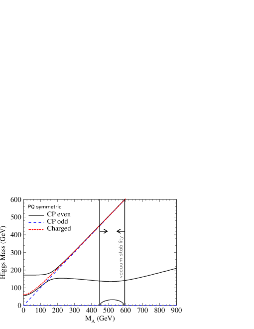
Figure 4: The one-loop Higgs boson masses, plotted as a function of $M_{A}$ for $\lambda=0.3$, $\kappa=0$, $v_{s}=3v$ and $\tan\beta=3$. The arrows denote the physically allowed region.

The five heavy Higgs bosons, $H_{3}$, $H_{2}$, $A_{2}$ and $H^{\pm}$, show a pattern very similar to the MSSM. However the spectrum is augmented by an additional massless pseudoscalar Goldstone boson and a very light scalar Higgs boson, conforming with the tree-level upper bound, $\lambda v\sin 2\beta/\sqrt{2}$, as evident from Eqn.(66). The positivity of the mass-squared of this additional scalar Higgs boson places a very stringent bound on the value of $M_{A}$, predicting a small bracket in analogy to Eqn.(36) for the $\kappa$ non-zero case, and consequently strongly constraining the masses of the Higgs bosons $H_{3}$, $A_{2}$ and $H^{\pm}$.

Taking $\lambda\to 0$, besides the massless pseudoscalar PQ axion, also the mass of the additional scalar Higgs boson approaches zero. Both fields decouple from the doublet Higgs sector. At the same time, however, the degenerate masses of the heavy Higgs bosons are fixed to the approximate value $M_{A}\approx\mu\tan\beta$. For $\kappa=0$, the “MSSM limit” is approached on a trajectory $\lambda\to 0$ that is constrained to a sheet in the MSSM parameter space that respects the PQ symmetry in the final MSSM potential. In fact, the $H_{u}H_{d}$ mixing term, that violates the PQ symmetry in the Higgs potential, is suppressed compared to the diagonal $|H_{u}|^{2}$ term, which respects the PQ symmetry, in the limit of large $M_{A}$ and $\tan\beta$ analyzed analytically above.

While the present model may serve as a nice illustration for the complex phenomena in the NMSSM, the presence of a massless pseudoscalar and light scalar rules out this parameter choice, due to their couplings to the $Z$ boson. The direct production of the lightest scalar together with a $Z$ boson, $Z\to ZH_{1}$, the coupling of which is shown in Fig.(5/left),

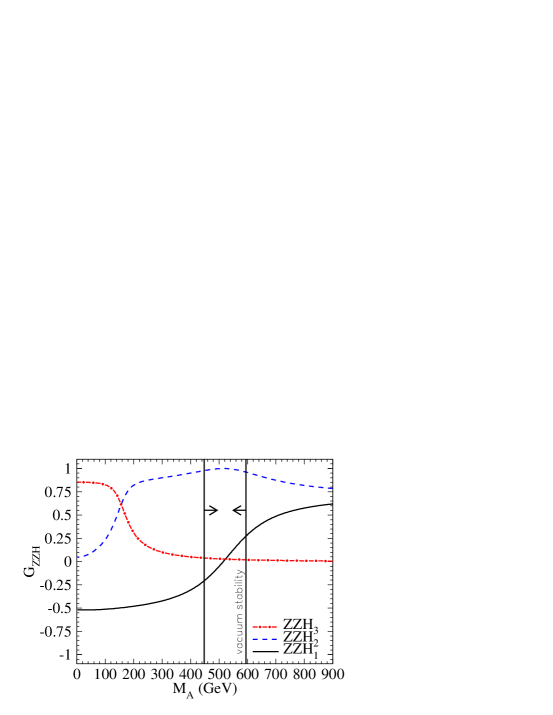
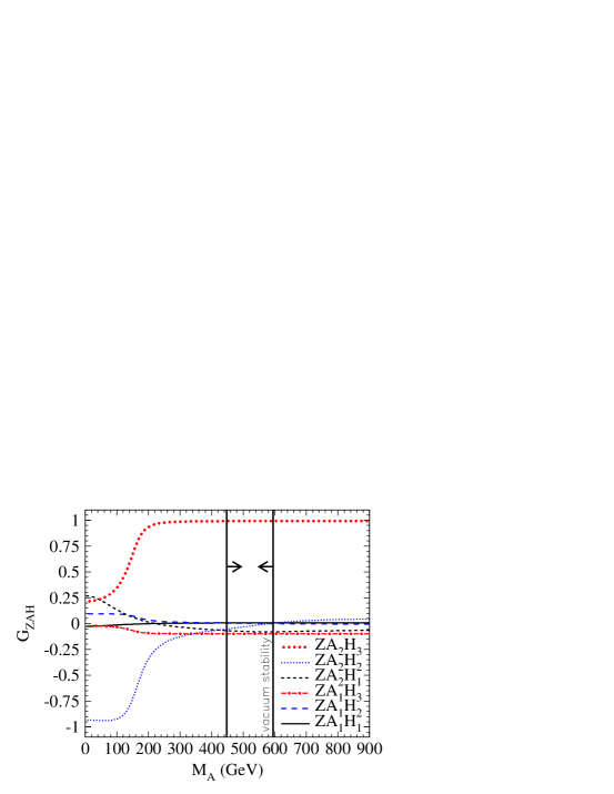
Figure 5: The couplings $\mathcal{G}_{ZZH_{i}}$ (left) and $\mathcal{G}_{ZA_{i}H_{j}}$ (right), plotted as a function of $M_{A}$ for $\lambda=0.3$, $\kappa=0$, $v_{s}=3v$ and $\tan\beta=3$. The arrows denote the physically allowed region.

would have been possible at LEP for much of the $M_{A}$ range. However, since the coupling passes through zero, such production alone does not yet rule out the model. The $Z$ boson decay $Z\to H_{1}A_{1}$ is more damaging, since the coupling $\mathcal{G}_{ZA_{1}H_{1}}$ (see Fig.(5/right)), although small, is always large enough to allow detection.

This may only be remedied by forcing $\lambda$ to become very small, so that the extra scalar and pseudoscalar fields decouple from the SM gauge bosons. Disregarding potential fine-tuning problems, these models are further constrained by astrophysical axion searches and cosmological bounds which are only satisfied for $10^{-10}<\lambda<10^{-7}$ [16]. Since $\mu$ is constrained to be of the order of the electroweak scale, this requires the extra singlet field to have a very large VEV, making this model unattractive as a solution to the $\mu$-problem.

3.3 The NMSSM with a slightly broken Peccei–Quinn symmetry

Turning on a non-zero value of $\kappa$ breaks the PQ $U(1)$ symmetry, providing a non-zero mass for the lightest pseudoscalar Higgs boson, and raising the mass of the lightest scalar Higgs boson. We consider the PQ symmetry to be only ‘slightly’ broken as long as $\kappa\ll 1$, for values of $v_{s}$ of the order of the electroweak scale. This is favoured by the renormalization group flow as illustrated in our earlier discussion. The model contains two extra parameters as compared to the case with an unbroken PQ symmetry: $\kappa$ and its associated soft SUSY breaking parameter $A_{\kappa}$.

As a representative example of this scenario we set $\lambda=0.3$ and $\kappa=0.1$. We will choose a value of $A_{\kappa}$ in the centre of the allowed range, $A_{\kappa}=-100$ GeV, c.f. Fig.(3), but the masses of the two singlet dominated fields can change significantly by altering this value.

The masses of the Higgs bosons for $\lambda=0.3$, $\kappa=0.1$, $v_{s}=3v$, $\tan\beta=3$ and $A_{\kappa}=-100$ GeV are shown as a function of $M_{A}$ in Fig.(6), including radiative corrections.

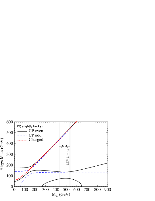
Figure 6: The one-loop Higgs boson masses as a function of $M_{A}$ for $\lambda=0.3$, $\kappa=0.1$, $v_{s}=3\,v$, $\tan\beta=3$ and $A_{\kappa}=-100$ GeV. The arrows denote the region allowed by LEP searches with 95% confidence.

The structure of the heavy Higgs boson masses, $H_{3}$, $A_{2}$ and $H^{\pm}$, remains very similar to the MSSM. However, the light Higgs boson mass spectrum is distinctly different, with two light scalar Higgs bosons and one light pseudoscalar Higgs boson. The extra singlet dominated pseudoscalar is no longer massless. Its mass has been raised from zero, by having the PQ symmetry explicitly broken by the term $\frac{1}{3}\kappa S^{3}$ in the superpotential, to a value largely independent of $M_{A}$, c.f. Eq.(30). Once again, the value of $M_{A}$ is bounded by the requirement that the vacuum be stable (i.e. $M^{2}_{H_{1}}>0$), although the restriction is now looser. The $H_{2}$ mass, of the order of $M_{Z}$ and largely independent of $M_{A}$, can rise above the canonical MSSM value due to the interaction with the new singlet fields, c.f. Eq(26). Generating a spectrum of light Higgs states, the NMSSM would be easily distinguished from the MSSM for this parameter range except in small regions where the $ZZH_{i}$ couplings are particularly close to zero.

Also shown are the restrictions on $M_{A}$ imposed by the LEP experiments [28] with 95% confidence. These limits are dependent on the masses of the light Higgs bosons and their couplings to the $Z$, as shown in Fig.(7).

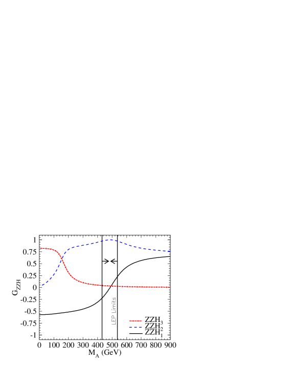
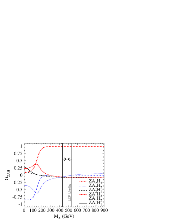
Figure 7: The couplings $\mathcal{G}_{ZZH_{i}}$ (left) and $\mathcal{G}_{ZA_{i}H_{j}}$ (right), as a function of $M_{A}$ for $\lambda=0.3$, $\kappa=0.1$, $v_{s}=3\,v$, $\tan\beta=3$ and $A_{\kappa}=-100$ GeV. The arrows denote the region allowed by LEP searches with 95% confidence.

The light scalar escapes detection via Higgs-strahlung only when it has a sufficiently reduced coupling to the $Z$ boson. Since this coupling passes through zero in the allowed range, one is unable to rule out all values of $M_{A}$. Furthermore, in contrast to the $\kappa=0$ scenario, the lightest pseudoscalar is now heavy enough to escape production via $e^{+}e^{-}\to H_{1}A_{1}$ at LEP. If the couplings of the lightest Higgs boson are particularly small, this could be difficult to discover even at the LHC. It is therefore important that a future linear collider, such as JLC/NLC/TESLA [30]–[32] or CLIC [33] perform a search for light Higgs bosons with reduced couplings.

Varying the parameters $v_{s}$ and $A_{\kappa}$ changes the quantitative, if not qualitative, features of the mass spectrum. In particular, large departures from the typical MSSM Higgs mass pattern occur in the light sector. As pointed out in Sec.(3.1), changing the value of $A_{\kappa}$ varies the lightest pseudoscalar and scalar masses while leaving the heavier Higgs bosons unaffected (see Fig. (3)).

If $v_{s}$ (or $\lambda$) is increased, all but the lightest Higgs boson become heavier. This can be seen in Fig.(8/left)

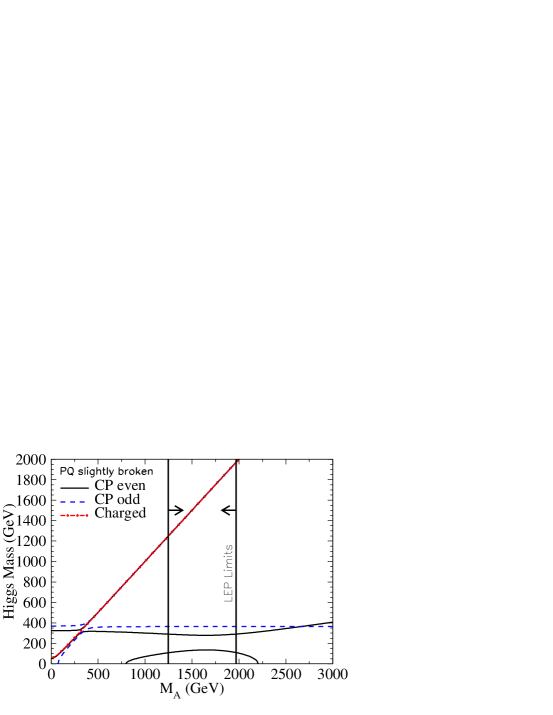
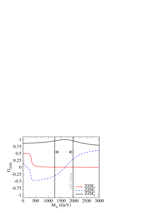
Figure 8: The one-loop Higgs boson masses(left) and couplings $\mathcal{G}_{ZZH_{i}}$ (right) as a function of $M_{A}$ for $\lambda=0.3$, $\kappa=0.1$, $v_{s}=10\,v$, $\tan\beta=3$ and $A_{\kappa}=-250$ GeV. The arrows denote the region allowed by LEP searches with 95% confidence.

where the Higgs boson masses have been plotted with $v_{s}=10\,v$, $A_{\kappa}=-250$ GeV and the other parameters as before. The restrictions on $M_{A}$ enforced by vacuum stability (i.e. $M_{H_{1}}^{2}>0$) are relaxed, allowing a larger range of $M_{A}$ values. One should note that $M_{A}\approx\sqrt{2}\lambda v_{s}/\sin 2\beta\approx\mu\tan\beta$ remains a point of particular interest as this choice allows the largest mass for $H_{1}$. $M_{A}$ is now forced to be beyond the $1$ TeV range.

Significantly, the increase of $v_{s}$ causes the mixing to become stronger, increasing the doublet component in $H_{1}$ at the expense of the doublet component in $H_{2}$. Consequently, the character of $H_{1}$ becomes more doublet-like, while the character of $H_{2}$ becomes more singlet-like. This increased mixing is quantified by Eqn.(40). Consequently, the lightest scalar Higgs boson acquires a significant coupling to the $Z$ boson, as shown in Fig.(8/right).

A further example of models in this class is given by $\lambda=0.05$, $\kappa=0.02$. Such a small value of $\lambda$ requires a large value of $v_{s}$, here taken to be $15\,v$, in order to satisfy the phenomenological constraints on $\mu$. The Higgs mass spectrum and couplings for this model remain qualitatively the same, as can be seen in Fig.(9), although a larger range of $M_{A}$ values remains viable.

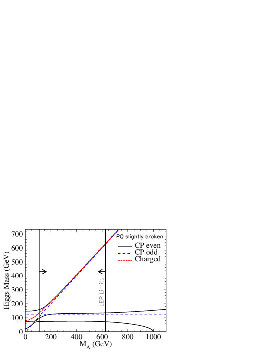
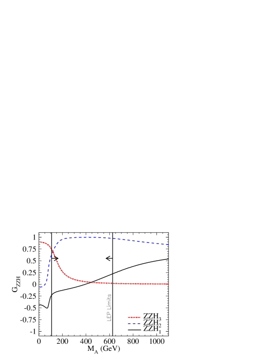
Figure 9: The one-loop Higgs boson masses (left) and couplings $\mathcal{G}_{ZZH_{i}}$ (right) as a function of $M_{A}$ for $\lambda=0.05$, $\kappa=0.02$, $v_{s}=15\,v$, $\tan\beta=3$ and $A_{\kappa}=-100$ GeV. The arrows denote the region allowed by LEP searches with 95% confidence.

Finally, changing the sign of $\kappa$, while keeping that of $\kappa A_{\kappa}$ fixed, results in behaviours very similar to their positive $\kappa$ counterparts. Changing the sign of $\kappa A_{\kappa}$ while keeping that of $\kappa$ fixed results in an unstable vacuum, as can be seen in Fig.(3).

3.4 The NMSSM with a strongly broken Peccei–Quinn symmetry

When $\kappa$ becomes large the PQ symmetry is strongly broken. This scenario has been shown earlier to be disfavoured by the renormalization group flow but cannot be ruled out a priori on general grounds. The parameters $v_{s}$, $M_{A}$ etc.  are taken to be of the order of the electroweak symmetry breaking scale. The extra pseudoscalar and scalar Higgs bosons gain moderately large masses from the PQ breaking term $\frac{1}{3}\kappa S^{3}$ in the superpotential, with values $M_{A_{1}}^{2}\sim-3\kappa v_{s}A_{\kappa}/\sqrt{2}$ and $M_{H_{2}}^{2}\sim\kappa v_{s}(\kappa v_{s}+\sqrt{2}A_{\kappa})/2$, c.f. Eqns.(30) and (32), largely independent of $M_{A}$. The eigenstate predominantly composed of the new scalar may in general no longer be the lightest scalar Higgs boson. That rôle is taken over by a Higgs boson which is predominantly composed of the doublet field $S_{2}$, with a mass of order $M_{H_{1}}\sim M_{Z}$ and a SM like coupling to the $Z$. The masses of these Higgs bosons are shown as a function of $M_{A}$ for the parameter choice $\lambda=0.3$, $\kappa=0.5$, $v_{s}=3\,v$, $\tan\beta=3$ and $A_{\kappa}=-500$ GeV, in Fig.(10).

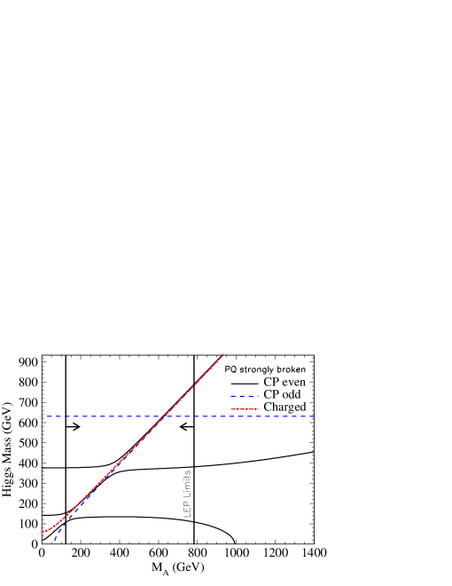
Figure 10: The one-loop Higgs boson masses as a function of $M_{A}$ for the parameter choice $\lambda=0.3$, $\kappa=0.5$, $v_{s}=3\,v$, $\tan\beta=3$ and $A_{\kappa}=-500$ GeV. The arrows denote the region allowed by LEP searches with 95% confidence.

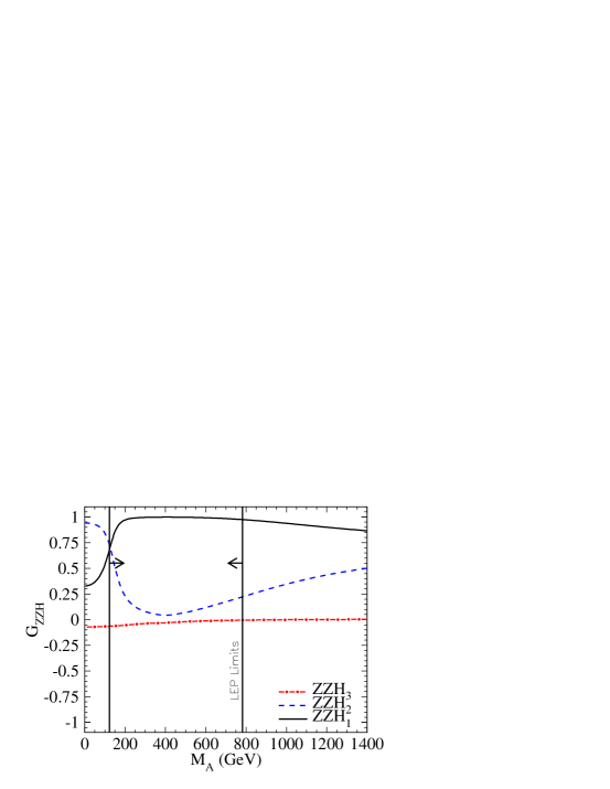
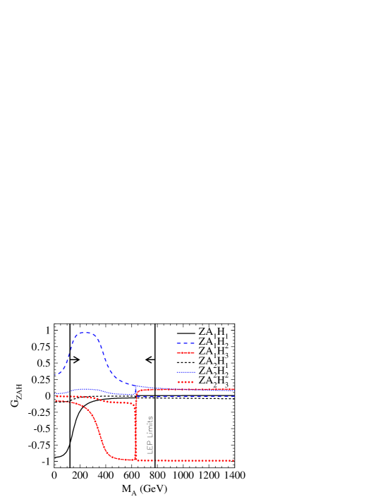
Figure 11: The couplings $\mathcal{G}_{ZZH_{i}}$ (left) and $\mathcal{G}_{ZA_{i}H_{j}}$ (right), as a function of $M_{A}$ for the parameter choice $\lambda=0.3$, $\kappa=0.5$, $v_{s}=3\,v$, $\tan\beta=3$ and $A_{\kappa}=-500$ GeV. The arrows denote the region allowed by LEP searches with 95% confidence.

Again the predominantly doublet fields follow the pattern of the MSSM, with one CP-even Higgs boson, $H_{1}$, below the electroweak scale and one CP-even, one CP-odd and two charged Higgs bosons nearly degenerate at the scale $M_{A}$. However, now the predominantly singlet scalar and pseudoscalar fields are heavy enough that they are no longer the lightest states for much of the physically allowed range, being, independently of $M_{A}$, at the scale of a few hundred GeV.

The couplings to the $Z$ boson, Fig.(11), show a complicated structure, due mainly to the way in which the Higgs states are labeled. As $M_{A}$ is increased a previously light Higgs boson may gain sufficient mass to overtake one of the other Higgs bosons. The labeling will change (according to the mass hierarchy) causing an apparent rapid variation of the $Z$ couplings at the crossing. It is this relabeling which gives the complicated structure of the $ZA_{i}H_{j}$ couplings.

Increasing the value of $v_{s}$ will increase the mass of the new fields substantially (since the effect of the increase seen in the previous section is magnified by the large value of $\kappa$). For example, with the same parameters as Fig.(10) except $v_{s}=10\,v$, the new scalar and pseudoscalar states have masses of the order of $1.6$ TeV and $1.2$ TeV, respectively, for all values of $M_{A}$ (although these masses show a strong dependence on $A_{\kappa}$). The new fields will also decouple, making the NMSSM very difficult to distinguish from the MSSM.

Once again, negative values of $\kappa$ do not change the qualitative picture as long as one also changes the sign of $A_{\kappa}$.

4 Summary and Conclusions

In this study, we have investigated the Higgs sector of the Next-to-Minimal Supersymmetric Standard Model, suggested by many GUT and superstring models. Moreover, this model attempts to explain the $\mu$-problem of the MSSM by introducing a new singlet Higgs field, $S$, with a non-zero vacuum expectation value. When this new field is coupled to the Higgs doublets, its expectation value leads to the $\mu$ term of the MSSM, providing a value of $\mu$ which may naturally be expected near the electroweak scale.

We have given expressions for the Higgs boson mass matrices and presented, besides the numerical analyses, approximate analytical solutions for the charged, CP-even and CP-odd Higgs boson masses which provide a nice insight into the mass hierarchies. It has been found that useful sum rules and inequalities for the mass parameters can be established and that the requirement of vacuum stability can place useful bounds on the mass parameters and couplings of the Lagrangian.

The renormalization group flow of the parameters $\lambda$ and $\kappa$ from the GUT scale down to the electroweak scale provide strong upper bounds on their values at the electroweak scale, where small $\kappa$ is favoured. The qualitative features of the Higgs boson masses are dependent on how strongly the PQ symmetry of the model is broken, quite accurately described by the approximate analytical solutions.

If the PQ symmetry is left explicitly unbroken in the Lagrangian (spontaneously broken by the structure of the vacuum), a massless Goldstone boson is present, the PQ axion. Additionally, this model contains two CP-even Higgs bosons with masses of the order of the electroweak scale or lower. As in the MSSM, the heavy fields, one CP-odd, one CP-even and two charged Higgs bosons, are nearly degenerate, Fig.(4). However, unlike the MSSM, the vacuum structure of the model constrains these heavy states to lie close in mass to $\mu\tan\beta$. Non-observation of the PQ axion rules out most of the allowed parameter space, only allowing scenarios with very low values of $\lambda$ and therefore very high VEVs for the new singlet field, which thereby do not provide a natural solution of the $\mu$-problem.

If the PQ symmetry is slightly broken, the qualitative pattern for the particle spectrum remains intact, except that the lightest CP-odd state acquires a mass of the order of the electroweak scale. Thus the model contains a heavy CP-even and CP-odd Higgs boson plus two heavy charged Higgs bosons which are all nearly degenerate in mass, similarly to the MSSM. However, besides the standard light CP-even Higgs boson, the spectrum is complimented by a pair of CP-even and CP-odd Higgs bosons with masses below the electroweak symmetry breaking scale, Fig.(6). The LEP limits on the lightest Higgs boson mass allow some of the parameter space to be ruled out. However, since the couplings to the $Z$ boson can be very much reduced, the NMSSM with a slightly broken PQ symmetry constitutes a valid scenario. Observing three light Higgs bosons, but no charged light Higgs boson, at future colliders would present an opportunity to distinguish the NMSSM with a softly broken PQ symmetry from the MSSM, even if the heavy states are inaccessible. It is therefore important that future colliders search for light scalar and pseudoscalar Higgs bosons with reduced couplings.

In contrast, a strongly broken PQ symmetry, though disfavoured by the flow of the couplings from the GUT scale down to the electroweak scale, could provide extra moderately heavy Higgs bosons, Fig.(10), which are only weakly coupled to the $Z$ boson. Such decoupled scenarios would be more difficult to distinguish from the MSSM.

Acknowledgments: The authors are grateful to S. Dedes, C. Hugonie, S. Moretti, H.B. Nielsen and V. Rubakov for fruitful discussions. RN is indebted to Alfred Töpfer Stiftung and to the DESY Laboratory for a scholarship during his stay in Hamburg (2001–2002). The work of RN was also supported by the Russian Foundation for Basic Research (RFBR), projects 00-15-96562 and 02-02-17379.

Appendix: An approximate solution

The CP–even mass matrix of Eqns.(23–28) does not lend itself easily to obtaining analytic expressions for the physical Higgs masses. However, reasonably simple expressions can be found by making an approximation, providing expressions which may be used to shed some light on the behaviour of the Higgs masses as the other parameters are varied.

To construct this approximate solution in the scalar sector we regard both $1/\tan\beta$ and $1/M_{A}$ as small parameters of magnitude $\approx\varepsilon$ [$M_{A}$ gauged by the generic electroweak scale]. Then, as long as neither $\kappa$, $\lambda$ nor the other scales become too large, we observe a hierarchical structure in the CP–even mass matrix of the form:

$$\{M^{2}_{ij}\}=M_{A}^{2}\left(\begin{array}[]{cc}A&\varepsilon C^{\dagger}\\ \varepsilon C&\varepsilon^{2}B\end{array}\right),$$ (67)

where $B$ is a $2\times 2$ matrix, $C$ is a column vector and $A$ is a scalar, all of order unity.

Performing an auxiliary unitary transformation defined by the matrix,

$$V^{\dagger}=\left(\begin{array}[]{cc}1-\frac{1}{2}\varepsilon^{2}\Gamma^{\dagger}\Gamma&-\varepsilon\Gamma^{\dagger}\\ \varepsilon\Gamma&11-\frac{1}{2}\varepsilon^{2}\Gamma\Gamma^{\dagger}\end{array}\right)+\mathcal{O}(\varepsilon^{4}),$$ (68)

with $\Gamma=C/A,$ the mass matrix takes block diagonal form:

$$VM^{2}V^{\dagger} = M_{A}^{2}\left(\begin{array}[]{cc}A+\varepsilon^{2}C^{\dagger}C/A&0\\ 0&\varepsilon^{2}(B-CC^{\dagger}/A)\end{array}\right)+\mathcal{O}(\varepsilon^{3})$$ (71)

$$= \left(\begin{array}[]{ccc}M_{11}^{2}+\frac{M_{13}^{4}}{M_{11}^{2}}&0&0\\ 0&M_{22}^{2}&M_{23}^{2}-\frac{M_{13}^{2}M_{12}^{2}}{M_{11}^{2}}\\ 0&M_{23}^{2}-\frac{M_{13}^{2}M_{12}^{2}}{M_{11}^{2}}&M_{33}^{2}-\frac{M_{13}^{4}}{M_{11}^{2}}\end{array}\right)+\mathcal{O}(\varepsilon^{3}),$$ (75)

where $M^{2}_{ij}$ are the entries of the CP–even mass matrix, Eqns.(23–28). Note that $M^{2}_{12}/M_{A}^{2}$ is actually $\mathcal{O}(\varepsilon^{3})$, so many terms can be neglected (and have been in the above).

$VM^{2}V^{\dagger}$ is now easily diagonalized to give the approximate CP–even Higgs boson masses:

$$M_{H_{3}}^{2} = M_{11}^{2}+\frac{M_{13}^{4}}{M_{11}^{2}},$$ (76)

$$M_{H_{2/1}}^{2} = \frac{1}{2}\left(M_{22}^{2}+M_{33}^{2}-\frac{M_{13}^{4}}{M_{11}^{2}}\pm\sqrt{\left(M_{22}^{2}-M_{33}^{2}+\frac{M_{13}^{4}}{M_{11}^{2}}\right)^{2}+4\left(M_{23}^{2}-\frac{M_{13}^{2}M_{12}^{2}}{M_{11}^{2}}\right)^{2}}\right).$$ (77)

The diagonalization matrix is given by

$$R=\left(\begin{array}[]{ccc}1&0&0\\ 0&\cos\theta_{H}&-\sin\theta_{H}\\ 0&\sin\theta_{H}&\cos\theta_{H}\end{array}\right)\hskip 8.5359pt{\rm with}\hskip 8.5359pt\tan\theta_{H}=\frac{M_{23}^{2}-\frac{M_{13}^{2}M_{12}^{2}}{M_{11}^{2}}}{M_{22}^{2}-M_{H_{1}}^{2}}.$$ (78)

Combining $R$ with the first rotation matrix $V$ gives us the matrix $O$ linking the states $S_{i}$ to the mass eigenstates (see Eqn.(41): $H=OS$):

$$O = R^{\dagger}V$$ (82)

$$= \left(\begin{array}[]{ccc}1-M_{13}^{4}/2M_{11}^{4}&M_{12}^{2}/M_{11}^{2}&M_{13}^{2}/M_{11}^{2}\\ -\left[M_{13}^{2}\sin\theta_{H}+M_{12}^{2}\cos\theta_{H}\right]/M_{11}^{2}&\phantom{-}\cos\theta_{H}&\sin\theta_{H}\left[1-M_{13}^{4}/2M_{11}^{4}\right]\\ \phantom{-}\left[M_{12}^{2}\sin\theta_{H}-M_{13}^{2}\cos\theta_{H}\right]/M_{11}^{2}&-\sin\theta_{H}&\cos\theta_{H}\left[1-M_{13}^{4}/2M_{11}^{4}\right]\end{array}\right).$$

This approximation works remarkably well, as can be seen in Fig.(12), where both the exact (numerical) solution and the approximate solution, Eqns.(76–77), for the one-loop CP–even Higgs masses are shown as a function of $M_{A}$ for the favoured parameter set of the slightly broken PQ symmetry, $\lambda=0.3$, $\kappa=0.1$, $v_{s}=3\,v$, $\tan\beta=3$ and $A_{\kappa}=-100$ GeV, introduced in Sec.(3.2). The exact and approximate solutions agree well as long as $M_{A}$ does not become too small.

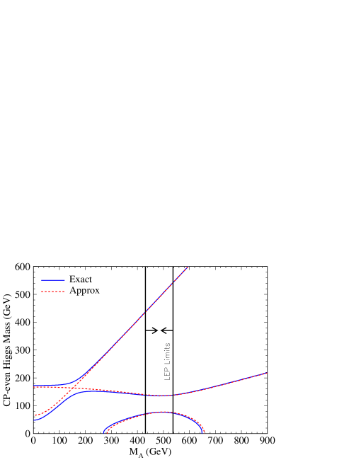
Figure 12: The exact (numerical) solution and the approximate solution for the one-loop CP–even Higgs masses as a function of $M_{A}$ for $\lambda=0.3$, $\kappa=0.1$, $v_{s}=3\,v$, $\tan\beta=3$ and $A_{\kappa}=-100$ GeV.

References

- [1] P. Ramond, Phys. Rev. D 3 (1971) 2415; A. Neveu and J. H. Schwarz, Nucl. Phys. B 31 (1971) 86; J. L. Gervais and B. Sakita, Nucl. Phys. B 34 (1971) 632; Y. A. Golfand and E. P. Likhtman, JETP Lett. 13 (1971) 323; [Pisma Zh. Eksp. Teor. Fiz. 13 (1971) 452]; J. Wess and B. Zumino, Nucl. Phys. B 70 (1974) 39; D. V. Volkov and V. P. Akulov, Phys. Lett. B 46 (1973) 109.
- [2] P. Fayet, Phys. Lett. B 64 (1976) 159; Phys. Lett. B 69 (1977) 489; Phys. Lett. B 84 (1979) 416; G. R. Farrar and P. Fayet, Phys. Lett. B 76 (1978) 575; E. Witten, Nucl. Phys. B 188 (1981) 513; S. Dimopoulos and H. Georgi, Nucl. Phys. B 193 (1981) 150; N. Sakai, Z. Phys. C 11 (1981) 153; H. P. Nilles, Phys. Rept. 110 (1984) 1; H. E. Haber and G. L. Kane, Phys. Rept. 117 (1985) 75; J. F. Gunion and H. E. Haber, Nucl. Phys. B 272 (1986) 1 [Erratum-ibid. B 402, 567 (1993)]; Nucl. Phys. B 278 (1986) 449; A. B. Lahanas and D. V. Nanopoulos, Phys. Rept. 145 (1987) 1.
- [3] E. Witten, Phys. Lett. B 105 (1981) 267; J. Polchinski and L. Susskind, Phys. Rev. D 26 (1982) 3661; S. Dimopoulos and H. Georgi, Nucl. Phys. B 193 (1981) 150; N. Sakai, Z. Phys. C 11 (1981) 153.
- [4] J. E. Kim and H. P. Nilles, Phys. Lett. B 138 (1984) 150.
- [5] M. Dine, W. Fischler and M. Srednicki, Phys. Lett. B 104 (1981) 199. H. P. Nilles, M. Srednicki and D. Wyler, Phys. Lett. B 120 (1983) 346; J. M. Frere, D. R. Jones and S. Raby, Nucl. Phys. B 222 (1983) 11; A. I. Veselov, M. I. Vysotsky and K. A. Ter-Martirosian, Sov. Phys. JETP 63 (1986) 489 [Zh. Eksp. Teor. Fiz. 90 (1986) 838].
- [6] J. P. Derendinger and C. A. Savoy, Nucl. Phys. B 237 (1984) 307;
- [7] U. Ellwanger, M. Rausch de Traubenberg and C. A. Savoy, Phys. Lett. B 315 (1993) 331.
- [8] S. F. King and P. L. White, Phys. Rev. D 52 (1995) 4183.
- [9] J. Ellis, J. F. Gunion, H. Haber, L. Roszkowski, F. Zwirner, Phys. Rev. D 39 (1989) 844.
- [10] U. Ellwanger, M. Rausch de Traubenberg and C. A. Savoy, Nucl. Phys. B 492 (1997) 21; F. Franke and H. Fraas, Int. J. Mod. Phys. A 12 (1997) 479; B. Ananthanarayan and P. N. Pandita, Int. J. Mod. Phys. A 12 (1997) 2321; U. Ellwanger and C. Hugonie, Eur. Phys. J. C 25 (2002) 297; U. Ellwanger, J. F. Gunion, C. Hugonie and S. Moretti, arXiv:hep-ph/0305109.
- [11] N. K. Falck, Z. Phys. C 30 (1986) 247;
- [12] L. J. Hall, J. Lykken and S. Weinberg, Phys. Rev. D 27 (1983) 2359; U. Ellwanger, Phys. Lett. B 133 (1983) 187; J. E. Kim and H. P. Nilles, Phys. Lett. B 138 (1984) 150; K. Inoue, A. Kakuto and H. Takano, Prog. Theor. Phys. 75 (1986) 664; A. A. Anselm and A. A. Johansen, Phys. Lett. B 200 (1988) 331; G. F. Giudice and A. Masiero, Phys. Lett. B 206 (1988) 480; L. J. Hall and L. Randall, Phys. Rev. Lett. 65 (1990) 2939; J. E. Kim and H. P. Nilles, Phys. Lett. B 263 (1991) 79; E. J. Chun, J. E. Kim and H. P. Nilles, Nucl. Phys. B 370 (1992) 105.
- [13] See, e.g. F. Zwirner, Int. J. Mod. Phys. A 3 (1988) 49, and references therein.
- [14] R. D. Peccei and H. R. Quinn, Phys. Rev. Lett. 38 (1977) 1440; Phys. Rev. D 16 (1977) 1791.
- [15] S. Weinberg, Phys. Rev. Lett. 40 (1978) 223; F. Wilczek, Phys. Rev. Lett. 40 (1978) 279.
- [16] For a review, see K. Hagiwara et al. [Particle Data Group Collaboration], Phys. Rev. D 66 (2002) 010001.
- [17] Y. B. Zeldovich, I. Y. Kobzarev and L. B. Okun, Zh. Eksp. Teor. Fiz. 67 (1974) 3 [Sov. Phys. JETP 40 (1974) 1].
- [18] A. Vilenkin, Phys. Rept. 121 (1985) 263; A. Vilenkin, E. P. S. Shellard, Cosmic Strings and Other Topological Defects (Cambridge University Press, 1994).
- [19] S. A. Abel, S. Sarkar and P. L. White, Nucl. Phys. B 454 (1995) 663; S. A. Abel, Nucl. Phys. B 480 (1996) 55.
- [20] C. Panagiotakopoulos and K. Tamvakis, Phys. Lett. B 446 (1999) 224; Phys. Lett. B 469 (1999) 145; A. Dedes, C. Hugonie, S. Moretti and K. Tamvakis, Phys. Rev. D 63 (2001) 055009.
- [21] C. Panagiotakopoulos and A. Pilaftsis, Phys. Rev. D 63 (2001) 055003;
- [22] H. M. Asatrian and G. K. Egiian, Mod. Phys. Lett. A 11 (1996) 2771; A. T. Davies, C. D. Froggatt and A. Usai, Phys. Lett. B 517 (2001) 375.
- [23] Y. Okada, M. Yamaguchi and T. Yanagida, Prog. Theor. Phys. 85 (1991) 1; J. Ellis, G. Ridolfi and F. Zwirner, Phys. Lett. B257 (1991) 83 and B262 (1991) 477; M. Carena, J. R. Espinosa, M. Quiros, C. Wagner, Phys. Lett. B355 (1995) 209; M. Carena, M. Quiros, C. Wagner, Nucl. Phys. B461 (1996) 407; J. A. Casas, J. R. Espinosa, M. Quiros, A. Riotto, Nucl. Phys. B436 (1995) 3.
- [24] P. A. Kovalenko, R. B. Nevzorov and K. A. Ter-Martirosian, Phys. Atom. Nucl. 61 (1998) 812 [Yad. Fiz. 61 (1998) 898].
- [25] R. B. Nevzorov and M. A. Trusov, Phys. Atom. Nucl. 64 (2001) 1513 [Yad. Fiz. 64 (2001) 1589].
- [26] R. B. Nevzorov and M. A. Trusov, Phys. Atom. Nucl. 64 (2001) 1299 [Yad. Fiz. 64 (2001) 1375]; Phys. Atom. Nucl. 65 (2002) 335 [Yad. Fiz. 65 (2002) 359].
- [27] B. Ananthanarayan and P. N. Pandita, Phys. Lett. B 371 (1996) 245.
- [28] The LEP Working Group for Higgs Boson Searches, LHWG Note/2001-03.
- [29] B.A. Dobrescu and K.T. Matchev, JHEP 0009 (2000) 031.
- [30] ACFA LC Working Group, K. Abe et al., KEK-REPORT-2001-11, hep-ex/0109166.
- [31] American LC Working Group, T. Abe et al., SLAC-R-570 (2001), hep-ex/0106055-58.
- [32] R. D. Heuer, D. J. Miller, F. Richard and P. Zerwas (eds.), TESLA: Technical Design Report (Part 3), DESY 010-11, hep-ph/0106315.
- [33] CLIC Study Team, R. W. Assman et al., CERN-2000-008.
- [34] E. Accomando et al., Phys. Rept. 299 (1998) 1; A. Djouadi, J. Kalinowski, P. Ohmann, P. M. Zerwas, Z. Phys. C74 (1997) 93.