$b-\tau$ UNIFICATION WITH GAUGINO
AND SFERMION MASS NON-UNIVERSALITY

Abstract

In the context of a SUSY GUT inspired MSSM version, the low energy consequences of the asymptotic $b-\tau$ Yukawa coupling Unification are examined, under the assumption of universal or non-universal boundary conditions for the gaugino and sfermion masses. Gaugino non-universality is applied, so that the SUSY corrections to $b$-quark mass can be reconciled with the present experimental data on muon anomalous magnetic moment. Restrictions on the parameter space, originating from the cold dark matter abundance in the universe, the inclusive branching ratio of $b\rightarrow s\gamma$ and the accelerator data are, also, investigated and the scalar neutralino-proton cross section is calculated. In the case of a bino-like LSP and universal boundary conditions for the sfermion masses, the constraints, arising from the cold dark matter and ${\rm BR}(b\to s\gamma)$ can be simultaneously satisfied, mainly thanks to the $A$-pole effect or the neutralino-stau coannihilations. In addition, sfermion mass non-universality provides the possibility of new coannihilation phenomena (neutralino-sbottom or neutralino-tau sneutrino-stau), which facilitate the simultaneous satisfaction of all the other requirements. In both cases above, the neutralino abundance can essentially decrease for a W-ino or higgsino like LSP creating regions of parameter space with additional neutralino-chargino and/or heavier neutralino coannihilations. The neutralino-sbottom mass proximity significantly ameliorates the detectability of LSP.

Keywords: Supersymmetric Models, Dark Matter
PACS codes: 12.60.Jv, 95.35.+d

Nucl. Phys. B678, 398 (2004)

1 INTRODUCTION

In some recent papers [1, 2], the early prediction in the context of $SU(5)$ Grand Unified Theory (GUT) [3] of the asymptotic $b-\tau$ Yukawa coupling Unification (YU) was beautifully combined with the present experimental data on neutrino physics within $SO(10)$ models. However, applying this scheme in the framework of the Constrained Minimal Supersymmetric (SUSY) Standard Model (CMSSM) [4] and given the top and tau experimental masses, the $\mu$ parameter is restricted to negative values [5, 6]. This is due to the fact that the tree level $b$-quark mass receives sizeable SUSY corrections [7], which can drive the corrected $b$-quark mass within its experimental range only for $\mu<0$. On the other hand, the $\mu<0$ case is in conflict with the present experimental data [8] on the muon anomalous magnetic moment [5, 6]. Indeed, the deviation, $\delta a_{\mu}$, of the measured value of the muon anomalous magnetic moment from its predicted value in the Standard Model (SM), seems to favor the $\mu>0$ regime [9, 10]. In addition, the negative sign of $\mu$ is severely restricted by the recent experimental results [11] on the inclusive branching ratio ${\rm BR}(b\rightarrow s\gamma)$ [5, 6], which bounds below the SUSY spectrum to rather high values.

At the same time, the SUSY spectrum can be bounded above by the requirement that the relic density, $\Omega_{\rm LSP}h^{2}$ of the lightest SUSY particle (LSP) in the universe does not exceed the upper limit on the Cold Dark Matter (CDM) abundance implied by cosmological considerations. After the recent experimental results of WMAP [12], this limit turns out to be as much stringent as the previous one (see, e.g. Ref. [13]) with a significantly better accuracy (see sec. 2.1). Since $\Omega_{\rm LSP}h^{2}$ increases with the LSP mass $m_{\rm LSP}$, this limit imposes a very strong upper bound on $m_{\rm LSP}$. However, this can significantly weaken in regions of the parameter space, where a substantial reduction of $\Omega_{\rm LSP}h^{2}$ can be achieved, mainly thanks to the $A$ pole effect ($A$PE) and/or the coannihilation mechanism (CAM). In the first case, which is applicable for large $\tan\beta$ [14, 15], the $\Omega_{\rm LSP}h^{2}$ reduction is caused by the presence of a resonance ($2m_{\rm LSP}\simeq m_{\rm A}$) in the $A$ mediated LSP’ s annihilation channel. On the other hand, CAM is activated for any $\tan\beta$, when a mass proximity occurs between the LSP and the next to LSP (NLSP). In the context of CMSSM, NLSP can be the lightest slepton [16, 17] and particularly stau [18, 15] for large $\tan\beta$ or stop [19, 20] for very large trilinear coupling, or also, chargino [21, 22]. Possible non-universality in the Higgs sector [23] gives rise to CAMs between LSP and $e$/$\mu$-sneutrino and/or chargino-sleptons.

As induced from the previous considerations, the viability of the $b-\tau$ YU hypothesis in the context of CMSSM becomes rather dubious. On the other hand, the embedding of MSSM into a $SU(5)$ or $SO(10)$ SUSY GUT leads, also, to a variety of possibilities [24] beyond the CMSSM universality. In this paper we will employ these scenaria in order to obtain SUSY spectra compatible with all these Cosmo-Phenomenological requirements. Namely non universal gaugino masses (UGMs) [25, 26] are applied, so that the inconsistency between the $\delta a_{\mu}$ constraint and the $b$-quark mass experimental data is removed. This effect can produce gaugino inspired CAMs (neutralino-chargino and/or heavier neutralino, $\mbox{$\tilde{\chi}$}-\mbox{${\tilde{\chi}_{2}^{\pm}}$}-\mbox{${\tilde{\chi}_{2}^{0}}$}$). On the other hand, new sfermionic CAMs (neutralino-sbottom, $\mbox{$\tilde{\chi}$}-\mbox{$\tilde{b}_{2}$}$ and neutralino-tau sneutrino-stau, $\mbox{$\tilde{\chi}$}-\mbox{$\tilde{\nu}_{\tau}$}-\mbox{$\tilde{\tau}_{2}$}$) can be caused by applying non universal sfermion masses (USFMs) [27, 28]. Both phenomena by themselves or in conjunction can drastically reduce $\Omega_{\rm LSP}h^{2}$ to an acceptably low level, increasing the upper bound on $m_{\rm LSP}$ almost up to $2~{}{\rm TeV}$. As a bonus, in both latter cases, the satisfaction of the BR($b\to s\gamma$) criterion is facilitated, allowing viable parameter space consistent even with the optimistic upper bound on $m_{\rm LSP}$ from $\delta a_{\mu}$ constraint (see sec. 2.5). Consequently the neutralino-proton cross sections are sensitively increased, especially in the case of $\mbox{$\tilde{\chi}$}-\mbox{$\tilde{b}_{2}$}$ CAM.

Combination of $b-\tau$ YU and non UGMs were previously considered in Refs. [25, 26], where, contrary to our case, a single dominant direction in gauge kinetic function has been assumed (see sec. 3). Additional presence of non USFMs were not studied until now, while the $\mbox{$\tilde{\chi}$}-\mbox{$\tilde{b}_{2}$}$ CAM was just noticed in Ref. [27]. Our main improvements are the consideration of the $\delta a_{\mu}$ constraint, the reproduction of the $\mbox{$\tilde{\chi}$}-\mbox{$\tilde{b}_{2}$}$ CAM in a much more restrictive framework, the finding of the $\mbox{$\tilde{\chi}$}-\mbox{$\tilde{\nu}_{\tau}$}-\mbox{$\tilde{\tau}_{2}$}$ CAM and the study of the co-existence of the gaugino inspired CAMs.

The framework of our analysis is described in some detail in sec. 2. The basic features of our model are established in sec. 3. Our numerical approach and results are exhibited in secs. 4 and 5. We end up with our conclusions and some open issues in sec. 6. Throughout the text and the formulas, brackets are used by applying disjunctive correspondence.

2 COSMO-PHENOMENOLOGICAL FRAMEWORK

We briefly describe the operation of the various Cosmo-Phenomenological criteria that we will use in our investigation. In the following formulas, gaugino masses, $M_{2},M_{3}$, top trilinear coupling $A_{t}$, $\mu$ parameter and the various SUSY corrections, $\Delta m_{b[\tau]}$ to $b$-quark [$\tau$-lepton] mass are calculated, at a SUSY breaking scale, $M_{\rm SUSY}$ specified in sec. 4.

2.1 COLD DARK MATTER CONSIDERATIONS

According to WMAP results [12], the total (M) and the baryonic (B) matter abundance in the universe is respectively:

$$\Omega_{\rm M}h^{2}=0.135_{-0.009}^{+0.008}~{}~{}\mbox{and}~{}~{}\Omega_{\rm B}h^{2}=0.0224\pm 0.0009.$$ (1)

We, thus, deduce the $95\%$ confidence level (c.l.) range for the CDM abundance [29]:

$$\Omega_{\rm CDM}h^{2}=0.1126_{-0.0181}^{+0.0161}.$$ (2)

In the context of MSSM, the lightest neutralino, $\tilde{\chi}$ can be the LSP. It consists the most natural candidate for solving the CDM problem, being neutral, weakly interacting and stable in the context of SUSY theories with $R$-Parity [30] conservation. Hence, in our analysis, we require the LSP relic density not to exceed the upper bound of Eq. (2):

$$\Omega_{\rm LSP}h^{2}\lesssim 0.13.$$ (3)

We calculate $\Omega_{\rm LSP}h^{2}$, using micrOMEGAs [31], which is one of the most complete publicly available codes. This includes accurately thermally averaged exact tree-level cross sections of all possible (co)annihilation processes, treats poles properly and uses one loop QCD corrections to the Higgs decay widths and couplings into fermions [32].

2.2 SCALAR NEUTRALINO-PROTON CROSS SECTION

Neutralinos could be detected via their elastic scattering with nuclei [33]. The quantity which is being conventionally used in the literature (e.g. [34, 35]) to compare experimental [36, 37] and theoretical results is the scalar neutralino-proton ($\mbox{$\tilde{\chi}$}-p$) cross section,

$$\sigma_{\tilde{\chi}p}^{\rm SI}=4\,\mu^{2}_{\tilde{\chi}p}f_{p}^{2}/\pi~{}~{}{\rm where}~{}~{}\mu_{\tilde{\chi}p}=m_{\rm LSP}m_{p}/(m_{\rm LSP}+m_{p})$$ (4)

and $f_{p}$ is the scalar contribution to the effective $\mbox{$\tilde{\chi}$}-p$ coupling. We calculate it, using the full one loop treatment of Ref. [35] (with some typos fixed [38]). This is indispensable for a reliable result in the region $m_{\rm LSP}\sim m_{\tilde{b}_{2}}$, where the tree level approximation (which, indeed works well elsewhere) fails. For the involved renormalization-invariant functions were adopted the values [34] (in the notation of Ref. [35]):

$$f_{{\rm T}_{u}}^{p}=0.02\pm 0.004,\qquad f_{{\rm T}_{d}}^{p}=0.026\pm 0.005,\qquad f_{{\rm T}_{s}}^{p}=0.118\pm 0.062.$$ (5)

Combining the sensitivities of the recent [36] and planned [37] experiments, we end in the following phenomenologically interesting region, for $100~{}{\rm GeV}\lesssim m_{\rm LSP}\lesssim 500~{}{\rm GeV}$:

$$\mbox{\sf a)}~{}~{}3\times 10^{-9}~{}{\rm pb}\lesssim\sigma_{\tilde{\chi}p}^{\rm SI}~{}~{}~{}~{}\mbox{and}~{}~{}~{}~{}\mbox{\sf b)}~{}~{}\sigma_{\tilde{\chi}p}^{\rm SI}\lesssim 2\times 10^{-6}~{}{\rm pb}$$ (6)

For SUSY spectra of our models consistent with all the other constraints of sec. 2, the obtained $\sigma_{\tilde{\chi}p}^{\rm SI}$ lies beyond the claimed by DAMA preferred range, $(1-10)\times 10^{-6}~{}\rm{pb}$, which however, has mostly been excluded by other collaborations (e.g. EDELWEISS, ZEPLIN I).

2.3 SUSY CORRECTIONS TO $b$-QUARK AND $\tau$-LEPTON MASS

In the large and intermediate $\tan\beta$ regime, the tree level $b$-quark mass, $m_{b}$ receives sizeable SUSY corrections [7, 39, 40], $\Delta m_{b}$ which arise from sbottom-gluino, $\left(\Delta m_{b}\right)^{\tilde{b}\tilde{g}}$ (mainly) and stop-chargino, $(\Delta m_{b})^{\tilde{t}\tilde{\chi}^{\pm}}$ loops. $(\Delta m_{b})^{\tilde{t}\tilde{\chi}^{\pm}}$ interferes destructively (see Eq. 12)) to $\left(\Delta m_{b}\right)^{\tilde{b}\tilde{g}}$ which, normally (an exception is constructed in Ref. [41]) dominates $\Delta m_{b}$. Consequently:

$${\rm sign}~{}\Delta m_{b}={\rm sign}~{}M_{3}\>\mu,~{}~{}\mbox{since}~{}~{}{\rm sign}~{}\left(\Delta m_{b}\right)^{\tilde{b}\tilde{g}[\tilde{t}\tilde{\chi}^{\pm}]}={\rm sign}~{}M_{3}~{}[A_{t}]\>\mu,$$ (7)

using the standard sign convention of Ref. [43]. Hence, for $M_{3}\mu>[<]~{}0$, the corrected $b$-quark mass at a low scale $M_{Z}$,

$$m^{\rm c}_{b}(M_{Z})=m_{b}(M_{Z})\left(1+\Delta m_{b}\right),$$ (8)

turns out to be above [below] its tree level value $m_{b}(M_{Z})$. The result is to be compared with the $95\%$ c.l. experimental range for $m^{\rm c}_{b}(M_{Z})$. This is derived by appropriately [44] evolving the corresponding range for the pole $b$-quark mass, $m_{b}(m_{b})$ up to $M_{Z}$ scale with $\alpha_{s}(M_{Z})\simeq 0.1185$, in accord with the analysis in Ref. [45]:

$$m_{b}(m_{b})=4.25\pm 0.3\>{\rm GeV}\>\>\>{\Longrightarrow}\>\>\>m^{\rm c}_{b}(M_{Z})=2.88\pm 0.2\>{\rm GeV}.$$ (9)

Less important but not negligible (almost 5$\%$) are the SUSY corrections to $\tau$-lepton, $\Delta m_{\tau}$ originated from [39] sneutrino-chargino, $\left(\Delta m_{\tau}\right)^{\tilde{\nu}_{\tau}\tilde{\chi}^{\pm}}$ (mainly) and stau-neutralino, $(\Delta m_{\tau})^{\tilde{\tau}\tilde{\chi}}$ loops, with the following signs:

$${\rm sign}~{}\Delta m_{\tau}=-{\rm sign}~{}M_{2}\>\mu,~{}~{}\mbox{since}~{}~{}{\rm sign}~{}\left(\Delta m_{\tau}\right)^{\tilde{\nu}_{\tau}\tilde{\chi}^{\pm}[\tilde{\tau}\tilde{\chi}]}=-{\rm sign}~{}M_{2}~{}[-M_{1}]\>\mu.$$ (10)

2.4 BRANCHING RATIO OF $b\rightarrow s\gamma$

Taking into account the recent experimental results [11] on this ratio, ${\rm BR}(b\rightarrow s\gamma)$, and combining appropriately the experimental and theoretical involved errors [44], we obtain the following $95\%$ c.l. range:

$$\mbox{\sf a)}~{}~{}1.9\times 10^{-4}\lesssim{\rm BR}(b\rightarrow s\gamma)~{}~{}~{}~{}\mbox{and}~{}~{}~{}~{}\mbox{\sf b)}~{}~{}{\rm BR}(b\rightarrow s\gamma)\lesssim 4.6\times 10^{-4}$$ (11)

We compute ${\rm BR}(b\rightarrow s\gamma)$ by using an updated version of the relevant calculation contained in the micrOMEGAs package [31]. In this code, the SM contribution is calculated using the formalism of Ref. [46] including the improvements of Ref. [47]. The $H^{\pm}$ contribution is evaluated by including the next-to-leading order (NLO) QCD corrections from Ref. [48] and $\tan\beta$ enhanced contributions from Ref. [49]. The dominant SUSY contribution, ${\rm BR}(b\rightarrow s\gamma)|_{\rm SUSY}$, includes resummed NLO SUSY QCD corrections from Ref. [49], which hold for large $\tan\beta$. The $H^{\pm}$ contribution interferes constructively with the SM contribution, whereas ${\rm BR}(b\rightarrow s\gamma)|_{\rm SUSY}$ interferes de[con]-structively with the other two contributions for $-M_{3}\mu<[>]~{}0$, since [42], in general:

$${\rm sign}~{}{\rm BR}(b\rightarrow s\gamma)|_{\rm SUSY}={\rm sign}~{}A_{t}\>\mu,~{}~{}\mbox{with}~{}~{}{\rm sign}~{}A_{t}=-{\rm sign}~{}M_{3}.$$ (12)

However, the SM plus $H^{\pm}$ contributions and the ${\rm BR}(b\rightarrow s\gamma)|_{\rm SUSY}$ decrease as $m_{\rm LSP}$ increases and so, a lower bound on $m_{\rm LSP}$ can be derived from Eq. (11a [11b]) for $M_{3}\mu>[<]~{}0$ with the latter being much more restrictive. It is obvious from Eqs. (12) and (7) that simultaneous combination of negative correction to $b$-quark mass and destructive contribution of ${\rm BR}(b\rightarrow s\gamma)|_{\rm SUSY}$ is impossible [42].

2.5 MUON ANOMALOUS MAGNETIC MOMENT

The deviation, $\delta a_{\mu}$ of the $a_{\mu}$ measured value from its predicted value in the SM, $a^{\rm SM}_{\mu}$ can be attributed to SUSY contributions, arising from chargino-sneutrino and neutralino-smuon loops. $\delta a_{\mu}$ is calculated by using micrOMEGAs routine based on the formulæof Ref. [50]. The absolute value of the result decreases as $m_{\rm LSP}$ increases and its sign is:

$${\rm sign}~{}\delta a_{\mu}={\rm sign}~{}M_{2}\>\mu.$$ (13)

On the other hand, the $a^{\rm SM}_{\mu}$ calculation is not yet stabilized mainly due to the instability of the hadronic vacuum polarization contribution. According to the evaluation of this contribution in Ref. [9], the findings based on $e^{+}e^{-}$ annihilation and $\tau$-decay data are inconsistent with each other. Taking into account these results and the recently announced experimental measurements [8] on $a_{\mu}$, we impose the following $95\%$ c.l. ranges:

$$\mbox{\sf a)}\hskip 16.95pt11.3\times 10^{-10}\lesssim\delta a_{\mu} \mbox{\sf b)}~{}~{}\delta a_{\mu}\lesssim 56.1\times 10^{-10}~{}~{}~{}~{}\mbox{$e^{+}e^{-}$-based}$$ and (14)

$$\vspace*{19pt}\mbox{\sf a)}~{}-11.6\times 10^{-10}\lesssim\delta a_{\mu} \mbox{\sf b)}~{}~{}\delta a_{\mu}\lesssim 30.4\times 10^{-10}~{}~{}~{}~{}\mbox{$\tau$-based}$$ and (15)

A lower bound on $m_{\rm LSP}$ can be derived for $M_{2}\mu>[<]~{}0$ from Eq. (14b [15a]) and an optimistic upper bound for $M_{2}\mu>0$ from Eq. (14a) which, however is not imposed as an absolute constraint due to the former computational instabilities. Although the $M_{2}\mu<0$ case can not be excluded [51], it is considered as quite disfavored [10], because of the poor $\tau$-decay data. For this reason, following the common practice [23, 29], we adopt the restrictions to parameters induced from Eq. (14).

2.6 COLLIDER BOUNDS

The relevant for our analysis is the $95\%$ c.l. LEP bound on the lightest CP-even neutral Higgs boson [52], $h$ and the lightest sbottom [53], $\tilde{b}_{2}$ mass,

$$\mbox{\sf a)}~{}~{}m_{h}\gtrsim 114.4~{}{\rm GeV}~{}~{}\mbox{and}~{}~{}\mbox{\sf b)}~{}~{}m_{\tilde{b}_{2}}\gtrsim 95~{}{\rm GeV}.$$ (16)

The SUSY corrections to $m_{h}$ are calculated at two-loop by using the FeynHiggsFast [54] program included in micrOMEGAs code [31].

3 PARTICLE MODEL

The embedding of MSSM in a SUSY GUT enriches the model with extra constraints and opens new possibilities beyond the CMSSM universality [24]. We below select some of them, constructing the Yukawa (sec. 3.1), gaugino (sec. 3.2) and scalar (sec. 3.3) sector of our theory. Actually, it is a variant of the models proposed in secs. II and III of Ref. [24]. The phenomenological reasons which push us in the introduction of the non-universalities of sec. 3.2 and 3.3 will become obvious during the presentation of our results in sec. 5. However, for clarity, let us outline them shortly. Consistency of $b-\tau$ YU with Eq. (14a) requires a proper application of non UGMs. The resulting model has still two shortcomings: (i) Uninteresting $\sigma_{\tilde{\chi}p}$ due to large minimal $m_{\rm LSP}$, since this is derived from Eq. (11b) (ii) Inability for the satisfaction of Eq. (14b). Non USFMs assist us to alleviate both disadvantages.

3.1 $b-\tau$ UNIFICATION

In the minimal $SU(5)$ SUSY GUT [24, 6], the third generation left handed superfields $L=(\nu_{\tau},\tau)$, $b^{c}$ belong to the ${\bf\bar{5}}$ representation (reps), while $Q=(t,b)$, $t^{c}$, $\tau^{c}$ belong to the ${\bf 10}$ reps. Assuming that the electroweak Higgs superfields $H_{1}$, $H_{2}$ are contained in ${\bf\bar{5}}_{H}$ and ${\bf 5}_{H}$ reps, respectively, the model predicts $b-\tau$ YU at GUT scale, $M_{\rm GUT}$ ($M_{\rm GUT}$ is determined by the requirement of gauge coupling unification):

$$h_{b}(M_{\rm GUT})=h_{\tau}(M_{\rm GUT})=y_{b\tau}$$ (17)

since, the Yukawa coupling terms of the resulting version of MSSM:

$$h_{b}H_{1}^{\mbox{\sf\scriptsize T}}i\tau_{2}Q\;b^{c}+h_{\tau}H_{1}^{\mbox{\sf\scriptsize T}}i\tau_{2}L\;\tau^{c}$$ (18)

originate from an unique term, $y_{b\tau}\ {\bf\bar{5}}\ {\bf 10}\ {\bf\bar{5}}_{H}$ of the underlying GUT.

The asymptotic relation of Eq. (17) can also arise in the context of $SO(10)$ SUSY GUT. In this case, a family of fermions is incorporated in the ${\bf 16}$ spinorial reps. Assuming that $H_{1}$, $H_{2}$ are contained in two different Higgses [24, 1] in ${\bf 10}_{H_{D}}$ and ${\bf 10}_{H_{U}}$, the terms in Eq. (18) can be again derived from an unique term, $y_{b\tau}\ {\bf 16}\ {\bf 16}\ {\bf 10}_{H_{D}}$. Alternatively, if $H_{1}$, $H_{2}$ are expressed as a combination of ${\bf 10}_{H}$ and ${\bf\overline{126}}_{H}$, large atmospheric neutrino mixing, produced through a non canonical see-saw mechanism, requires [2] $b-\tau$ YU.

Assuming exact $b-\tau$ YU at $M_{\rm GUT}$ and given the top and tau masses, $\tan\beta$ and $m^{\rm c}_{b}(M_{Z})$ can not be both free parameters (see, also, sec. 4). We choose as input parameter in our presentation $m^{\rm c}_{b}(M_{Z})$ (in contrast with the usual in the literature strategy, see, e.g. Refs. [5, 6, 25, 26]). As a consequence, a prediction can be made for $\tan\beta$. Furthermore, the sign of $\Delta m_{b}$ has to be negative. This is, because close to the complete YU ($\tan\beta\;\simeq 50$), we obtain $m_{b}(M_{Z})$ close to the upper edge of the range of Eq. (9). As $\tan\beta$ decreases, $m_{b}(M_{Z})$ increases [55] and so, a negative $\Delta m_{b}$ can drive $m^{\rm c}_{b}(M_{Z})$ for some values of $\tan\beta<50$ (see, e.g. Fig. 4 of Ref. [56]) within the above range. Combining this result with Eq. (7), we conclude that $b-\tau$ YU can become viable only for $M_{3}\mu<0$ (in accordance with the findings of Refs. [5, 6, 25, 26]).

3.2 GAUGINO SECTOR

From the discussion of the previous section, we can induce that $b-\tau$ YU in the context of CMSSM [4], is viable only for $\mu<0$. Consequently the parameter space of the model can be restricted through Eq. (15), which, however, is rather oracular. To liberate the model from this ugly feature, we invoke a departure from the UGMs. The importance of non UGMs in addressing the former inconsistency has already been stressed in Refs. [25, 26]. Indeed, from Eqs. (7) and (13), we can infer that negativity of $\Delta m_{b}$ and positivity of $\delta a_{\mu}$, can be reconciled with the following arrangement:

$$M_{1}(M_{\rm GUT}):M_{2}(M_{\rm GUT}):M_{3}(M_{\rm GUT})=1:+[-]r_{2}:-[+]r_{3},~{}~{}\mbox{with}~{}~{}\mu>[<]~{}0,$$ (19)

and $r_{2},r_{3}>0$. Such a condition can arise, by employing a moderate deviation from the minimal Supergravity (mSUGRA) scenario [58, 59, 60, 61, 62] (for an other approach see, e.g. Refs. [57]) as follows.

According to the gravity-mediated SUSY breaking mechanism [64], gaugino masses $M_{i},i=1,2,3$ are generated by a left handed chiral superfield $\Phi$, which appears linearly in the gauge kinetic function $f_{\alpha\beta}$ ($\alpha,\beta$ run over the GUT gauge group generators). During the spontaneous breaking of the GUT symmetry, auxiliary fields $F_{\Phi}$, components of $\Phi$, coupled to gauginos, acquire vacuum expectation values (vevs), which can be considered as the asymptotic $M_{i}$. In mSUGRA models, the fields $F_{\Phi}$ are treated as singlets under the underlying GUT and therefore, UGMs result. However, $F_{\Phi}$ can belong to any reps $r$ in the symmetric product ($\rm S$) of two adjoints [58]. Thus, after the breaking of the GUT symmetry to the SM one, $F^{r}_{\Phi}$ acquire vevs in the SM neutral direction $\langle F^{r}_{\Phi}\rangle_{\alpha\beta}=n^{r}_{\alpha}\delta_{\alpha\beta}$, where $n^{r}_{\alpha}$ are group theoretical factors. Therefore, the gaugino masses at $M_{\rm GUT}$ can be parameterized as follows ($i<\alpha$):

$$M_{i}(M_{\rm GUT})=M_{1/2}\sum_{r}c_{r}n_{i}^{r},$$ (20)

where $M_{1/2}$ is a gaugino mass parameter and the characteristic numbers $n_{i}^{r}$ of every reps $r$ have been worked out in Ref. [63] for the $SU(5)$ and in Ref. [65] for the $SO(10)$ GUT. Also, $c_{r}$ are the relative weight of the reps $r$ in the sum. They can be treated as free parameters, while there is no direct experimental constraint on the resulting signs [60]. As emphasized in Refs. [59, 24], all the cases are compatible with the gauge coupling unification with the assumption that the scalar component of $\Phi$ develops negligible vev. One can next show, by solving the resulting 3x3 systems (we ignore for simplicity the large reps 220 [770] for $SU(5)~{}[SO(10)]$), that there is a wide and natural set of $c_{r}$ ’s in Eq. (20) for $0<r_{2,3}<2$, so that the ratio of Eq. (19) can be realized. To keep our investigation as general as possible, we will not assume (as usually [25, 59, 65]) dominance of a specific direction in Eq. (20). Nevertheless, we will comment on these more restrictive but certainly more predictive cases, in the conclusions.

We will close this section, quoting several important comments:

i. In both cases of Eq. (19), ${\rm BR}(b\rightarrow s\gamma)|_{\rm SUSY}$ interferes constructively to SM+$H^{\pm}$ contribution and therefore, the satisfaction of Eq. (11b) has to be attained.

ii. The renormalization group running is affected very little by the specific choice one of the two possibilities in Eq. (19). However, we choose to work with $\mu>0$, since in this case the resulting value of $\tan\beta$ is slightly diminished. This is due to the fact that for $\mu>0$, $\Delta m_{\tau}$ increases (due to the additive correlation of the two contributions in Eq. (10) which does not exist for $\mu<0$ with $M_{2}<0$ from Eq. (19)). As a consequence, with given the tau yukawa coupling $h_{\tau}(M_{\rm SUSY})$, a larger $m_{\tau}(M_{\rm SUSY})$ (or smaller $\tan\beta$) for $\mu>0$ is needed so as a successful $m_{\tau}(M_{Z})$ is obtained (see, also, sec. 4).

iii. For $r_{2}>1$ and $r_{3}>1$, LSP is mainly a pure B-ino. However for $r_{2}<1$ and/or $r_{3}<1$, LSP can become W-ino or Higgsino like and the mass of charginos and/or gluinos decrease so as they can coannihilate with LSP reducing $\Omega_{\rm LSP}h^{2}$ even lower than the expectations [72]. Despite the fact that $\Omega_{\rm LSP}h^{2}$ much lower than the bound of Eq. (2) can not be characterized as a fatal disadvantage of the theory (since other production mechanisms of LSP may be activated [73] and/or other CDM candidates may contribute to $\Omega_{\rm CDM}h^{2}$) we will keep our investigation in regions of $r_{2},r_{3}$, where $\Omega_{\rm LSP}h^{2}$ turns out to be close to the bound of Eq. (2) for $m_{\rm LSP}<2~{}{\rm TeV}$.

3.3 SCALAR SECTOR

In the minimal $SU(5)$ SUSY GUT [67, 24], the soft SUSY breaking terms for the sfermions in ${\bf 10}$ reps ($\tilde{Q}=(\tilde{t},\tilde{b})$, $\tilde{t}^{c}$, $\tilde{\tau}^{c}$), $m_{\bf 10}$ and in ${\bf\bar{5}}$ reps ($\tilde{L}=(\tilde{\nu}_{\tau},\tilde{\tau})$, $\tilde{b}^{c}$), $m_{\bf\bar{5}}$ can be different. Consequently, the soft SUSY breaking masses for the sfermions of the resulting MSSM at $M_{\rm GUT}$ can be written as:

$$m_{\tilde{Q}}^{2}(M_{\rm GUT})=m_{\tilde{t}^{c}}^{2}(M_{\rm GUT})=m_{\tilde{\tau}^{c}}^{2}(M_{\rm GUT}) = m_{0}^{2},$$ (21)

$$m_{\tilde{L}}^{2}(M_{\rm GUT})=m_{\tilde{b}^{c}}^{2}(M_{\rm GUT}) = r^{2}_{\tilde{f}}m_{0}^{2},~{}~{}0<r^{2}_{\tilde{f}}<2$$ (22)

where we have adopted the parameterization and the range for $r^{2}_{\tilde{f}}$ of Refs. [68, 27]. Similar splitting between sfermion masses can also occur in the context of $SO(10)$ [69, 24, 28] although in the presence of some $D$-terms. To suppress dangerous flavor changing neutral currents [70], we maintain the universality among generations. Remarkably, such a non-universality among sleptons can be probed at $e^{+}e^{-}$ colliders [71]. As we will see in sec. 5, $r^{2}_{\tilde{f}}<1$ can decrease considerably the resulting masses of $\tilde{b}_{2}$ and $\tilde{\nu}_{\tau}$ so as to have a chance to play the rôle of coannihilator during the LSP freeze out in the Early Universe, reducing efficiently $\Omega_{\rm LSP}h^{2}$.

As regards the soft masses of the two higgses $H_{1},H_{2}$, included in ${\bf\bar{5}}_{H}~{}[{\bf 5}_{H}]$, they can be in general arbitrary (even in the case of $SO(10)$ SUSY GUT since we assumed two higgses ${\bf 10}_{H_{U}},{\bf 10}_{H_{D}}$ in sec. 3.1)

$$m_{H_{1}}^{2}(M_{\rm GUT})=r^{2}_{H_{1}}m_{0}^{2}~{}~{}\mbox{and}~{}~{}m_{H_{2}}^{2}(M_{\rm GUT})=r^{2}_{H_{2}}m_{0}^{2},~{}~{}0<r^{2}_{H_{1},H_{2}}<2$$ (23)

However, trying to isolate the non USFMs and reduce the number of the free parameters, we will restrict ourselves to the simplificative case $r_{H_{1}}=r_{H_{2}}=1$. Nevertheless, we will comment on the conclusion how this assumption can influence our results.

4 NUMERICAL CALCULATION

In our numerical calculation, we closely follow the notation as well as the renormalization group and radiative electroweak symmetry breaking (RESB) analysis of Refs. [44]. We integrate the 2-loop renormalization group equations (RGEs) for the gauge and Yukawa coupling constants and 1-loop for the soft SUSY breaking terms between $M_{\rm GUT}$ and a common SUSY threshold $M_{\rm SUSY}\simeq(m_{\tilde{t}_{1}}m_{\tilde{t}_{2}})^{1/2}$ ($\tilde{t}_{1,2}$ are the stop mass eigenstates) determined in consistency with the SUSY spectrum. At $M_{\rm SUSY}$ we impose RESB, evaluate the SUSY spectrum and incorporate the SUSY corrections to $b$ and $\tau$ masses [39, 40]. Between $M_{\rm SUSY}$ and $M_{Z}$, the running of gauge and Yukawa couplings is continued using the SM RGEs.

We use fixed values for the running top quark mass $m_{t}(m_{t})=166~{}{\rm GeV}$ and tau lepton mass $m_{\tau}(M_{Z})=1.746~{}{\rm{GeV}}$. Using an iterative up-down approach, $h_{t}(M_{\rm GUT})$ and $h_{\tau}(M_{\rm GUT})$ are determined for each $\tan\beta$ at $M_{\rm SUSY}$, while $h_{b}(M_{\rm GUT})$ is derived from the $b-\tau$ YU assumption, Eq. (17). Equivalently, turning the procedure around, $\tan\beta$ can be adjusted so, that the derived $h_{b}(M_{\rm GUT})$ corresponds to a desired $m^{\rm c}_{b}(M_{Z})$. Fixing it, also, to its central experimental value of Eq. (9), $m^{\rm c}_{b}(M_{Z})=2.88~{}{\rm GeV}$, a prediction for $\tan\beta$ can be made, as already mentioned in sec. 3.1. Finally, we impose the boundary conditions given by Eqs. (19) with $\mu>0$ for the gaugino masses, by Eqs. (21)-(23) for the scalar masses and we also, assume a universal trilinear scalar coupling, $A_{0}$.

In summary, our effective theory below $M_{\rm GUT}$ depends on the parameters :

$$M_{1/2},~{}m_{0},~{}A_{0},~{}r_{2},~{}r_{3},~{}r_{\tilde{f}}.$$

To further reduce the parameter space of the model, we fix (as usually [15, 23, 29]) $A_{0}=0$. $A_{0}\neq 0$ is not expected to change dramatically our results. Also, for presentation purposes, $M_{1/2}$ and $m_{0}$ can be replaced by $m_{\rm LSP}$ and a relative mass splitting, $\Delta_{\rm P}$, defined as follows:

$$\Delta_{\rm P}=\left\{\matrix{(m_{\rm P}-2m_{\rm LSP})/2m_{\rm LSP}\hfill,&\mbox{if}~{}~{}{\rm P}:A\hfill\cr(m_{\rm P}-m_{\rm LSP})/m_{\rm LSP}\hfill,&\mbox{if}~{}~{}{\rm P}:\mbox{$\tilde{\tau}_{2}$},\mbox{$\tilde{b}_{2}$}~{}\mbox{or}~{}\mbox{$\tilde{\nu}_{\tau}$}\hfill\cr}\right.$$ (24)

The choice of this parameter is convenient, since it determines, for given $m_{\rm LSP}$, the strength of the $A$PE for P : $A$ or of the CAM for P : $\mbox{$\tilde{\tau}_{2}$},\mbox{$\tilde{b}_{2}$}~{}\mbox{and}~{}\mbox{$\tilde{\nu}_{\tau}$}$. It, thus, essentially unifies the description of both reduction “procedures” (see sec. 5). Note that although $\Delta_{\tilde{\chi}^{\pm}_{2}}~{}[\Delta_{\tilde{\chi}^{0}_{2}}]$ can be defined through a relation similar to this in the second line of Eq. (24) with P : $\tilde{\chi}^{\pm}_{2}~{}[\tilde{\chi}^{0}_{2}]$, these can not be used in order to determine the spectrum, since they depend crucially only on $M_{1/2}$ and not on $m_{0}$. So, they vary very slowly, once $r_{2}$ or $r_{3}$ have been chosen. Consequently, our final set of the considered free parameters is:

$$m_{\rm LSP},\ \Delta_{\rm P},\ r_{2},\ r_{3},\ r_{\tilde{f}}.$$

5 RESULTS

We proceed, now in the delineation of the parameter space of our model. For the sake of illustration, we divide this section in subsections devoted to each applied $\Omega_{\rm LSP}h^{2}$ reduction “procedure”. The CAMs are classified to 3 main categories based to the sfermionic ones with or without the presence of $\mbox{$\tilde{\chi}$}-\mbox{${\tilde{\chi}_{2}^{\pm}}$}-\mbox{${\tilde{\chi}_{2}^{0}}$}$ CAMs. In this case, the allowed ranges of the basic parameters $m_{\rm LSP},\Delta_{\rm P}$ and $\tan\beta$ are listed comparatively in the Tables 1, 2, 3 together with the relative contributions beyond a threshold value of the (co)annihilation processes to the $\Omega_{\rm LSP}h^{2}$ calculation as $m_{\rm LSP}$ and $\Delta_{\tilde{\tau}_{2}}$ vary in their allowed (or, indicative in some cases) ranges. The allowed regions on the $m_{\rm LSP}-\Delta_{\rm P}$ plane from the various absolute constraints of sec. 2 are shaded, while the regions favored by the optimistic upper bound of Eq. (14a) are ruled. For simplicity, we do not show bounds from constraints less restrictive than those which are crucial.

Let us introductionary explain the reasons for which we will focus on some specific $r_{2},r_{3}$ and $r_{\tilde{f}}$. Initially, in order to make contact with the highly predictive and well-investigated parameter space of CMSSM (see, e.g. Refs. [19, 21, 22, 17, 29]) we will consider $r_{2}=r_{3}=r_{\tilde{f}}=1$. Indeed, for $r_{2}=r_{3}=1$, the resulting low energy values of the soft SUSY breaking terms turn out to be quite similar to those that we would have obtained, if we had imposed UGMs with $\mu<0$. The gaugino running (see, e.g. Ref. [66]) and essentially, the LSP gaugino purity, $G_{P}$ (in the notation of Ref. [66]), remain unaltered. The scalar running is altered by a few percent due to the resulting lower values of the trilinear couplings. This is, because their running crucially depends on the relative sign of $M_{2}$ and $M_{3}$. The latter difference has the following remarkable consequences. In our case: (i) $\Delta m_{b}$ turns out to be larger. This is because, $\left(\Delta m_{b}\right)^{\tilde{t}\tilde{\chi}^{\pm}}$ anti-correlates more weakly with $\left(\Delta m_{b}\right)^{\tilde{b}\tilde{g}}$ due to lower $|A_{t}|$ (sec. 2.3). (ii) $\tan\beta$ is significantly decreased (especially in the case of universal sfermion masses), since the tree level $m_{b}(M_{Z})$ has to be larger (sec. 3.1), so that after the subtraction of the larger $\Delta m_{b}$, the resulting $m^{\rm c}_{b}(M_{Z})$ is within its experimental margin of Eq. (9). (iii) ${\rm BR}(b\rightarrow s\gamma)$ is lower, since ${\rm BR}(b\rightarrow s\gamma)|_{\rm SUSY}$ and the $H^{\pm}$ contribution is diminished, mainly due [49] to the larger denominator of the resummation and lower $\tan\beta$ enhanced contributions, respectively.

For $r_{2}=r_{3}=1$ and $r_{\tilde{f}}=1,0.2,0.4$, we will present the mass parameters and the allowed regions on the $m_{\rm LSP}-\Delta_{\rm P}$ plane. Possible variation of $r_{2},r_{3}$ is not expected to change the general characteristics of the mass parameters. Also, we checked that $r_{2}>1$ and/or $r_{3}>1$ do not create new CAMs and so, do not essentially deform the allowed regions. However, for $r_{2}<1$ and/or $r_{3}<1$, additional CAMs can further enlarge them. A first example will be given for $r_{2}=0.6$ and $r_{3}=1$. With this choice, $\Delta_{\tilde{\chi}^{\pm}_{2}}\sim 0.1$ is established, creating a background of useful (not very drastic) $\mbox{$\tilde{\chi}$}-\mbox{${\tilde{\chi}_{2}^{\pm}}$}-\mbox{${\tilde{\chi}_{2}^{0}}$}$ CAMs (in accord with Ref. [72]) which can be combined with the sfemionic ones. However, essential reduction of $G_{P}$ is obtained only for $r_{3}<1$. For $r_{2}=1$ and $r_{3}<1$, new situation for the $\Omega_{\rm LSP}h^{2}$ calculation emerges for $r_{3}<0.5$. Then, $\Delta_{\tilde{\chi}^{\pm}_{2}}<0.1$ and $\mbox{$\tilde{\chi}$}-\mbox{${\tilde{\chi}_{2}^{\pm}}$}-\mbox{${\tilde{\chi}_{2}^{0}}$}$ CAMs reduce $\Omega_{\rm LSP}h^{2}$ lower than the expectations. Instead, we will insist on the choice, $r_{2}=0.6$ and $r_{3}=0.5$ or 0.6, for which $\mbox{$\tilde{\chi}$}-\mbox{${\tilde{\chi}_{2}^{\pm}}$}-\mbox{${\tilde{\chi}_{2}^{0}}$}$ CAMs can be kept under control.

Finally, let the hadronic inputs of Eq. (5) vary within their ranges we will derive the corresponding bands on the $m_{\rm LSP}-\sigma_{\tilde{\chi}p}^{\rm SI}$ plane for various $\Delta_{\rm P}$ and $r_{2}=r_{3}=r_{\tilde{f}}=1$, while possible improvement for $r_{2}<1$ and $r_{3}<1$ will be illustrated, too. The findings will be collectively presented in Fig. 5, but the explanations will be given separately in each subsection.

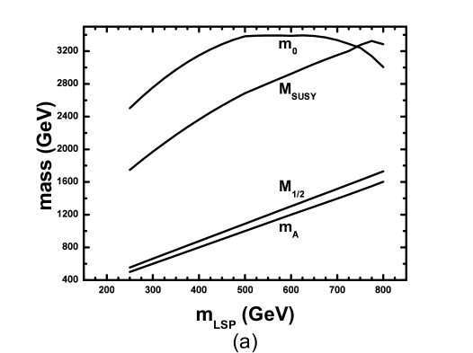
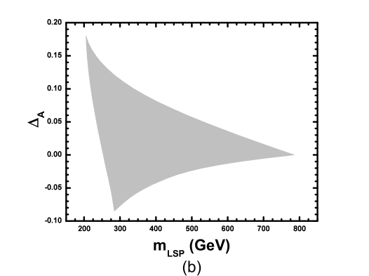
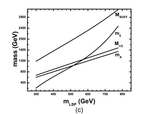
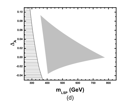
Figure 1: For $r_{\tilde{f}}=r_{2}=r_{3}=1$ and high [low] $m_{0}$, the mass parameters $M_{1/2}$, $m_{0}$, $m_{A}$ and $M_{\rm SUSY}$ versus $m_{\rm LSP}$ for $\Delta_{A}=0$ (a [c]) and the allowed (shaded) area on the $m_{\rm LSP}-\Delta_{A}$ plane (b [d]). Ruled is, also, the area favored by the optimistic upper bound on $m_{\rm LSP}$ from Eq. (14a)

5.1 $A$-POLE EFFECT (WITH OR WITHOUT $\mbox{$\tilde{\chi}$}-\mbox{${\tilde{\chi}_{2}^{\pm}}$}-\mbox{${\tilde{\chi}_{2}^{0}}$}$ COANNIHILATIONS)

For $r_{2}=r_{3}=1$ and $0<r_{\tilde{f}}\leq 1.2$, reduction of $\Omega_{\rm LSP}h^{2}$ caused by the $A$PE is possible. Especially, for $r_{\tilde{f}}=1$, there are two different combinations of $M_{1/2}$ and $m_{0}$, which support this possibility. In Figs. 1-(a) and 1-(c), we present the mass parameters $M_{1/2}$, $m_{0}$, $m_{A}$ and $M_{\rm SUSY}$ versus $m_{\rm LSP}$ for $\Delta_{A}=0$ in these two cases. We observe that the main difference between them is related to the value of $m_{0}$, which turns out to be relatively high [low] in Fig. 1-(a [c]). In these, the various lines terminate at low [high] $m_{\rm LSP}$’s due to improper RESB ($m_{A}^{2}<0$) [$m^{\rm c}_{b}(M_{Z})$].

The corresponding allowed areas on the $m_{\rm LSP}-\Delta_{A}$ plane are displayed in Figs. 1-(b) and 1-(d). In both cases, the left (almost vertical) boundary of the allowed (shaded) region comes from Eq. (11b) while the lower and upper curved boundaries correspond to the saturation of Eq. (3). A simultaneous satisfaction of Eq. (14a) is impossible. More explicitly, we find the following allowed ranges:

$${\bf i.}~{}~{}205~{}[284]~{}{\rm GeV}\lesssim m_{\rm LSP}\lesssim 784~{}{\rm GeV}~{}~{}\mbox{for}~{}~{}0.18~{}\left[|-0.085|\right]\gtrsim\left|\Delta_{A}\right|\gtrsim 0,$$ (25)

with $45~{}[45.2]\gtrsim\tan\beta\gtrsim 41.2$ in the high $m_{0}$ case (Fig. 1-(b)). Saturation of the optimistic bound from Eq. (14a) is not possible in the overall investigated parameter space.

$${\bf ii.}~{}~{}357~{}[405]~{}{\rm GeV}\lesssim m_{\rm LSP}\lesssim 775~{}{\rm GeV}~{}~{}\mbox{for}~{}~{}0.093~{}[|-0.036|]\gtrsim\left|\Delta_{A}\right|\gtrsim 0$$ (26)

with $36~{}[35.2]\lesssim\tan\beta\lesssim 39.8$ in the low $m_{0}$ case (Fig. 1-(d)). The bound of Eq. (14a) implies $m_{\rm LSP}\lesssim 372~{}{\rm GeV}$.

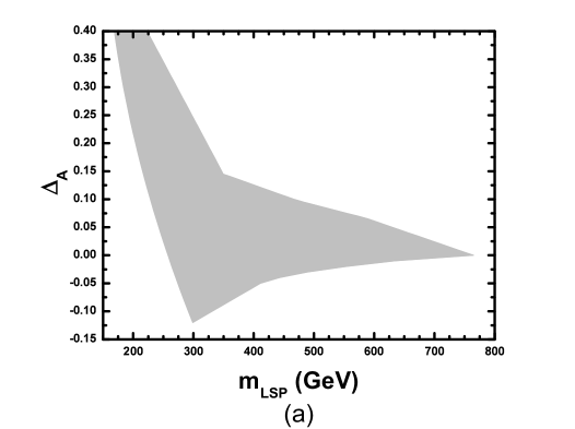
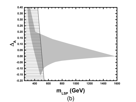
Figure 2: The allowed (shaded) area on the $m_{\rm LSP}-\Delta_{A}$ plane for $r_{\tilde{f}}=1,r_{2}=0.6,r_{3}=1$ and high $m_{0}$ (a), $r_{\tilde{f}}=0.4,r_{2}=r_{3}=0.6$ and low $m_{0}$ (b). Ruled is, also, the area favored by the optimistic upper bound on $m_{\rm LSP}$ from Eq. (14a).

Comparing Figs. 1-(b) and 1-(d), we observe that the allowed area for low $m_{0}$ can be included in this for high $m_{0}$, with the lower and upper curved boundaries being almost identical. The main difference is that the bound from Eq. (11b) is more restrictive in the low $m_{0}$ case, due to the lighter stop spectrum. This difference is also shown in Fig. 5-(a), where we depict $\sigma_{\tilde{\chi}p}^{\rm SI}$ versus $m_{\rm LSP}$ for $\Delta_{A}=0.1$ and low [high] $m_{0}$ (grey [light grey]) band. Obviously the high $m_{0}$ is phenomenologically more attractive.

Coexistence of $A$PE and $\mbox{$\tilde{\chi}$}-\mbox{${\tilde{\chi}_{2}^{\pm}}$}-\mbox{${\tilde{\chi}_{2}^{0}}$}$ CAM can further enlarge the allowed areas. Indeed, analyzing two cases, we find

$${\bf i^{\prime}.}~{}~{}299~{}{\rm GeV}\lesssim m_{\rm LSP}\lesssim 765~{}{\rm GeV}~{}~{}\mbox{for}~{}~{}|-0.12|\gtrsim\left|\Delta_{A}\right|\gtrsim 0,$$ (27)

with $35.5\lesssim\tan\beta\lesssim 37.2$ and high $m_{0}$ for $r_{\tilde{f}}=1,r_{2}=0.6$ and $r_{3}=1$ (Fig. 2-(a)) without possibility of saturation of the optimistic bound from Eq. (14a). The obtained $\sigma_{\tilde{\chi}p}^{\rm SI}$ turns out to be quite similar to this of light grey band in Fig. 5-(a).

$${\bf ii^{\prime}.}~{}~{}483.5~{}{\rm GeV}\lesssim m_{\rm LSP}\lesssim 1570~{}{\rm GeV}~{}~{}\mbox{for}~{}~{}|-0.156|]\gtrsim\left|\Delta_{A}\right|\gtrsim 0$$ (28)

with $35\lesssim\tan\beta\lesssim 39.4$ and low $m_{0}$ for $r_{\tilde{f}}=0.4$ and $r_{2}=r_{3}=0.6$ (Fig. 2-(b)). The bound of Eq. (14a) can be satisfied for $m_{\rm LSP}\lesssim 538~{}{\rm GeV}$ due to low $r_{\tilde{f}}$. The corresponding $\sigma_{\tilde{\chi}p}^{\rm SI}$ is also increased due to stronger higgsino component of the LSP as is shown in Fig. 5-(a), cyan band.

Due to the existence of the $\mbox{$\tilde{\chi}$}-\mbox{${\tilde{\chi}_{2}^{\pm}}$}-\mbox{${\tilde{\chi}_{2}^{0}}$}$ CAM, in both latter (i^′, ii^′) cases, there is no upper [lower] bound on $\Delta_{A}~{}[m_{\rm LSP}]$, for $\Delta_{A}>0$, contrary to the former cases (i, ii). Evident is, also, in any case that the $\Omega_{\rm LSP}h^{2}$ reduction, because of the $A$PE, is more efficient for $\Delta_{A}>0$ than for $\Delta_{A}<0$, in accord with the findings of Ref. [74].

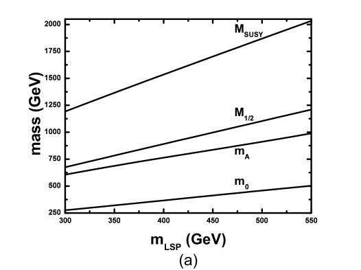
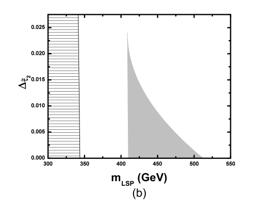
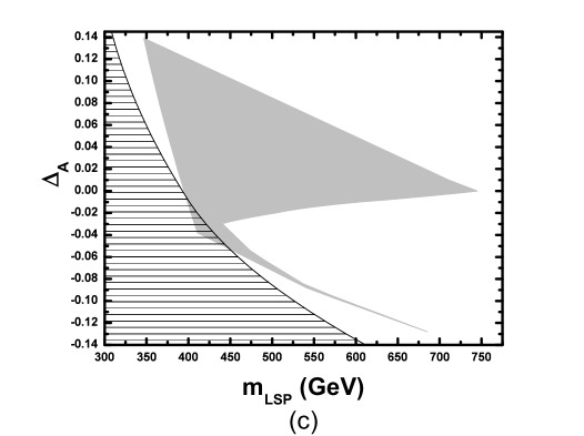
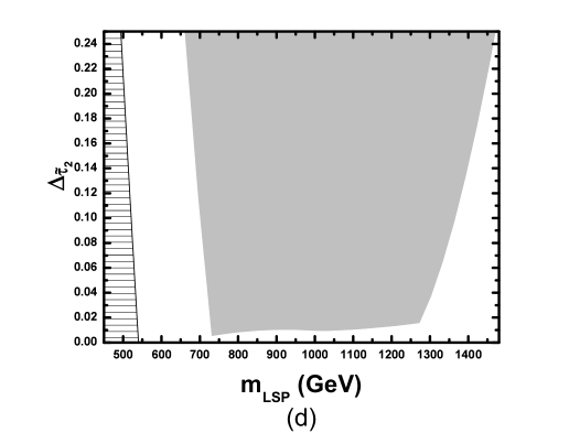
Figure 3: The mass parameters $M_{1/2}$, $m_{0}$, $m_{A}$ and $M_{\rm SUSY}$ versus $m_{\rm LSP}$ for $r_{\tilde{f}}=r_{2}=r_{3}=1$ and $\Delta_{\tilde{\tau}_{2}}=0$ (a) and the allowed (shaded) area for $r_{\tilde{f}}=1$ and $r_{2}=1~{}[0.6],r_{3}=1~{}[0.5]$ (b [d]) on the $m_{\rm LSP}-\Delta_{\tilde{\tau}_{2}}$ plane or $r_{\tilde{f}}=1$ and $r_{2}=0.6,r_{3}=1$ on the $m_{\rm LSP}-\Delta_{A}$ plane (c). Ruled is, also, the area favored by the optimistic upper bound on $m_{\rm LSP}$ from Eq. (14a).

In both cases, the relative contributions beyond 5$\%$ of the (co)annihilation processes to $\Omega_{\rm LSP}h^{2}$ as $m_{\rm LSP}$ and $\Delta_{A}$ vary in the ranges of Eq. (25) or (26) [(27) or (28)], are:

$\mbox{$\tilde{\chi}$}\mbox{$\tilde{\chi}$}\rightarrow b\bar{b}$	$(87-86)~{}[52-78]\%$
$\mbox{$\tilde{\chi}$}\mbox{$\tilde{\chi}$}\rightarrow\tau\bar{\tau}$	$(12.5-14)~{}[7-13]\%$

If we had imposed UGMs with $\mu<0$ and $r_{\tilde{f}}=1$, the high $m_{0}$ case would not have survived, due to larger $\tan\beta$ which would have invalidated the RESB, while for low $m_{0}$, we could have found allowed area similar to this in Fig. 2-(b) with $m_{\rm LSP}\gtrsim 466~{}{\rm GeV}$ and $\tan\beta\simeq 42$.

5.2 $\mbox{$\tilde{\chi}$}(-\mbox{${\tilde{\chi}_{2}^{\pm}}$}-\mbox{${\tilde{\chi}_{2}^{0}}$})-\mbox{$\tilde{\tau}_{2}$}$ COANNIHILATIONS

The most usual and easily achieved (for $r_{\tilde{f}}\neq 1$, also) CAM is the $\mbox{$\tilde{\chi}$}-\mbox{$\tilde{\tau}_{2}$}$ CAM. The mass parameters $M_{1/2}$, $m_{0}$, $m_{A}$ and $M_{\rm SUSY}$ which support this situation, are plotted versus $m_{\rm LSP}$ for $\Delta_{\tilde{\tau}_{2}}=0$ and $r_{\tilde{f}}=r_{2}=r_{3}=1$ in Fig. 3-(a). We observe that $M_{1/2}\gg m_{0}$, unlike all the other cases.

The corresponding allowed area on the $m_{\rm LSP}-\Delta_{\tilde{\tau}_{2}}$ plane, for the same $r$ ’s is depicted in Fig. 3-(b) and it turns out to be disconnected from these of subsec. 5.1. The left (almost vertical) [right curved] boundary of the allowed (shaded) region is derived from Eq. (11b  [3]). It is obvious that strong degeneracy among LSP and NLSP is needed in order the criteria of Eqs. (3) and (11b) to be simultaneously fulfilled without a possible achievement of Eq. (14a), since it implies $m_{\rm LSP}\lesssim 343~{}{\rm GeV}$ (Table 1, left column). Consequently, the corresponding $\sigma_{\tilde{\chi}p}^{\rm SI}$ lies also well below the range of Eq. (6b), as shown in Fig. 5-(b), dark grey band.

Table 1: DOMINANT CONTRIBUTIONS TO $\Omega_{\rm LSP}h^{2}$

MODEL PARAMETERS
$r_{\tilde{f}}$	$1$	$1$	$1$
$r_{2},r_{3}$	$r_{2}=r_{3}=1$	$r_{2}=0.6,r_{3}=1$	$r_{2}=0.6,r_{3}=0.5$
ALLOWED RANGES
$\tan\beta$	$35$	${\it 34.1}-35.1$	$34.2-{\it 39.4}$
$m_{\rm LSP}~{}({\rm GeV})$	$408-512$	${\it 400}-686$	$734-{\it 1420}$
$\Delta_{\tilde{\tau}_{2}}$	$0.15-0$	${\it 0.25}-0$	$0.01-{\it 0.25}$
PROCESSES WHICH CONTRIBUTE MORE THAN $7\%$
PROCESS	CONTRIBUTION ($\%$)
$\mbox{$\tilde{\chi}$}\mbox{$\tilde{\chi}$}\rightarrow b\bar{b}$	$40-2$	$82-0$	$-$
$\mbox{$\tilde{\chi}$}\mbox{$\tilde{\chi}$}\rightarrow\tau\bar{\tau}$	$8-1$	$13-0$	$-$
$\mbox{$\tilde{\chi}$}\mbox{$\tilde{\chi}$}\rightarrow W^{+}W^{-}$	$-$	$-$	$7-0$
$\tilde{\chi}\tilde{\tau}_{2}\rightarrow\tau\gamma$	$11-13$	$-$	$-$
$\tilde{\tau}_{2}\tilde{\tau}_{2}\rightarrow\tau\tau$	$10.5-32$	$0-12$	$-$
$\tilde{\tau}_{2}\tilde{\tau}_{2}^{\ast}\rightarrow\gamma\gamma$	$3-9.6$	$-$	$-$
$\tilde{\tau}_{2}\tilde{\tau}_{2}^{\ast}\rightarrow\gamma Z$	$1.6-7$	$-$	$-$
$\tilde{\tau}_{2}\tilde{\tau}_{2}^{\ast}\rightarrow b\bar{b}$	$12-18$	$0-18$	$-$
$\tilde{\tau}_{2}\tilde{\tau}_{2}^{\ast}\rightarrow t\bar{t}$	$-$	$0-16$	$-$
$\mbox{$\tilde{\chi}$}\mbox{${\tilde{\chi}_{2}^{+}}$}\rightarrow f_{u}\bar{f}_{d}$	$-$	$-$	$16.5-27$
$\mbox{${\tilde{\chi}_{2}^{+}}$}\mbox{${\tilde{\chi}_{2}^{-}}$}\rightarrow f_{u}\bar{f}_{d}$	$-$	$-$	$0-12$
$\mbox{${\tilde{\chi}_{2}^{0}}$}\mbox{${\tilde{\chi}_{2}^{+}}$}\rightarrow f_{u}\bar{f}_{d}$	$-$	$-$	$0-15$

These “pessimistic” results are not essentially alleviated, lifting the UGMs. Indeed, for $r_{\tilde{f}}=1,r_{2}=0.6$ and $r_{3}=1$ the allowed area is somehow enlarged to higher $m_{\rm LSP}$ due to extra CAMs, but the lower $m_{\rm LSP}$ is still high enough to be phenomenologically interesting (Table 1, middle column, italic numbers are referred to indicative and not absolute bounds). In this case the $\mbox{$\tilde{\chi}$}-\mbox{$\tilde{\tau}_{2}$}$ coannihilation tail turns out to be connected to the allowed region caused by $A$PE. So, for economy, they are collectively presented on the $m_{\rm LSP}-\Delta_{A}$ plane in Fig. 3-(c). On the other hand, for $r_{\tilde{f}}=1,~{}r_{2}=0.6$ and $r_{3}=0.5$, an unusual behavior on the $m_{\rm LSP}-\Delta_{\tilde{\tau}_{2}}$ plane is presented in Fig. 3-(d). There, $\mbox{$\tilde{\chi}$}-\mbox{${\tilde{\chi}_{2}^{\pm}}$}-\mbox{${\tilde{\chi}_{2}^{0}}$}$ CAM are more efficient than the $\mbox{$\tilde{\chi}$}-\mbox{$\tilde{\tau}_{2}$}$. Strengthening the $\mbox{$\tilde{\chi}$}-\mbox{$\tilde{\tau}_{2}$}$ proximity, the $\mbox{$\tilde{\chi}$}-\mbox{${\tilde{\chi}_{2}^{\pm}}$}-\mbox{${\tilde{\chi}_{2}^{0}}$}$ CAM contribution to $\Omega_{\rm LSP}h^{2}$ decreases (Table 1, right column). So, $\Omega_{\rm LSP}h^{2}$ increases due to the domination of the weaker $\mbox{$\tilde{\chi}$}-\mbox{$\tilde{\tau}_{2}$}$ CAM and a lower bound on the $m_{\rm LSP}-\Delta_{\tilde{\tau}_{2}}$ plane emerges.

It is worth mentioning, that had we assumed UGMs with $\mu<0$ and $r_{\tilde{f}}=1$, the lower bound on $m_{\rm LSP}$, derived again from Eq. (11b), would have been much more restrictive ($m_{\rm LSP}\gtrsim 519~{}{\rm GeV}$ for $\tan\beta\simeq 40.6$). An explanation is given in the introduction of sec. 5. Thus, we would have been practically left without allowed area.

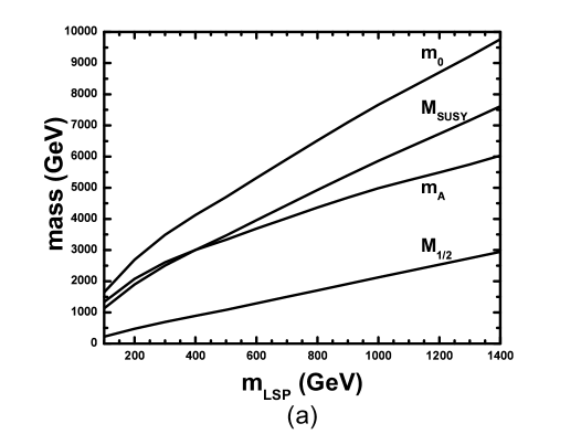
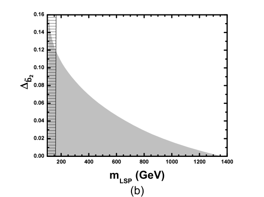
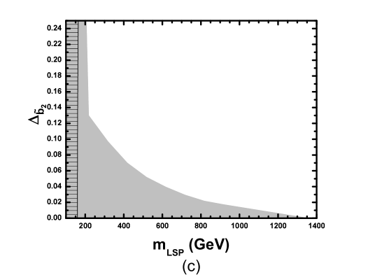
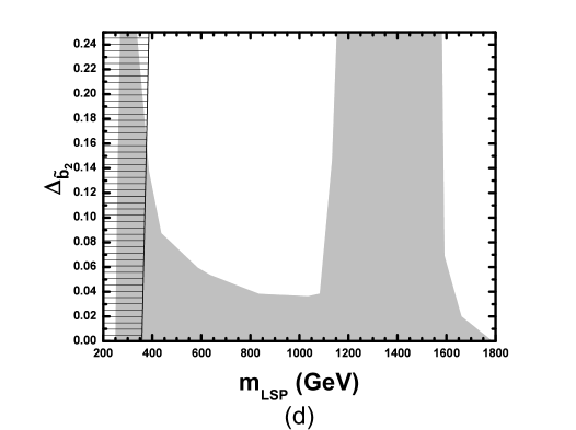
Figure 4: The mass parameters $M_{1/2}$, $m_{0}$, $m_{A}$ and $M_{\rm SUSY}$ versus $m_{\rm LSP}$ for $r_{\tilde{f}}=0.4,r_{2}=r_{3}=1$ and $\Delta_{\tilde{b}_{2}}=0$ (a) and the allowed (shaded) area on the $m_{\rm LSP}-\Delta_{\tilde{b}_{2}}$ plane for $r_{\tilde{f}}=0.4$ and $r_{2}=r_{3}=1$ (b), $r_{2}=0.6,r_{3}=1$ (c), $r_{2}=0.6,r_{3}=0.5$ (d). Ruled is, also, the area favored by the optimistic upper bound on $m_{\rm LSP}$ from Eq. (14a).

5.3 $\mbox{$\tilde{\chi}$}(-\mbox{${\tilde{\chi}_{2}^{\pm}}$}-\mbox{${\tilde{\chi}_{2}^{0}}$})-\mbox{$\tilde{b}_{2}$}$ COANNIHILATIONS

For moderate to low $r_{\tilde{f}}$, a new type of CAM between $\tilde{\chi}$ and $\tilde{b}_{2}$ can be obtained. However, the needed mass proximity can be established only for $M_{1/2}\ll m_{0}$, with $m_{0}>1~{}{\rm TeV}$ (in accord with the findings of Ref. [27]). This is, because $m_{\tilde{Q}}$ and $m_{\tilde{b}^{c}}$ [$m_{\tilde{L}}$ and $m_{\tilde{\tau}^{c}}$] de[in]-crease as $m_{0}$ increases, since $h_{t}$ and $h_{b}$ [$h_{\tau}$] in[de]-crease with the running from $M_{\rm GUT}$ to $M_{Z}$ [66]. Therefore, $m_{\tilde{b}_{2}}~{}[m_{\tilde{\tau}_{2}}]$ de[in]-creases drastically. So, $\tilde{b}_{2}$, which is mainly $\tilde{b}^{c}$ (unlike the similar case of Ref. [27]), can become coannihilator of $\tilde{\chi}$.

A typical example for the values of $M_{1/2}$, $m_{0}$, $m_{A}$ and $M_{\rm SUSY}$ versus $m_{\rm LSP}$ in this case, is presented in Fig. 4-(a) for $\Delta_{\tilde{b}_{2}}=0$ and $r_{\tilde{f}}=0.4$ and $r_{2}=r_{3}=1$. The resulting allowed area on the $m_{\rm LSP}-\Delta_{\tilde{b}_{2}}$ plane for the same $r$’s is displayed in Fig. 4-(b). The left (almost vertical) [right curved] boundary of the allowed (shaded) region is derived from Eq. (16a [3]). The bound of the right curve can be occasionally relaxed for $r_{2}<1$ and/or $r_{3}<1$. Two examples are depicted in Fig. 4-(c [d]) for $r_{\tilde{f}}=0.4$ and $r_{2}=0.6,r_{3}=1~{}[0.5]$. Due to extra CAMs there are regions without upper bound on $\Delta_{\tilde{b}_{2}}$. However the left (almost vertical) boundary becomes gradually more restrictive derived, in these cases, from Eq. (11b). Our findings are in detail and comparatively listed in Table 2 (recall that the italic numbers are refereed to indicative bounds). Optimistic bounds on $m_{\rm LSP}$ derived from Eq. (14a) are included in parenthesis.

It should be emphasized that the reduction of $\Omega_{\rm LSP}h^{2}$ caused by $\mbox{$\tilde{\chi}$}-\mbox{$\tilde{b}_{2}$}$ CAM is much more efficient than this by $\mbox{$\tilde{\chi}$}-\mbox{$\tilde{\tau}_{2}$}$ and $\mbox{$\tilde{\chi}$}-\mbox{$\tilde{\nu}_{\tau}$}-\mbox{$\tilde{\tau}_{2}$}$ CAM. As a consequence, larger $m_{\rm LSP}$’s (and $\Delta_{\tilde{b}_{2}}$’s) are allowed. It is also always constructive to and stronger than a possible $\mbox{$\tilde{\chi}$}-\mbox{${\tilde{\chi}_{2}^{\pm}}$}-\mbox{${\tilde{\chi}_{2}^{0}}$}$ CAM (for the used $r$ ’s) contrary to the case of $\mbox{$\tilde{\chi}$}-\mbox{${\tilde{\chi}_{2}^{\pm}}$}-\mbox{${\tilde{\chi}_{2}^{0}}$}-\mbox{$\tilde{\tau}_{2}$}$ CAM (sec. 5). At the same time, thanks to heavier stop and higgs sector, the satisfaction of Eq. (11b) is facilitated and there is parameter space where the putative bound of Eq. (14a) can be fulfilled, too.

Table 2: DOMINANT CONTRIBUTIONS TO $\Omega_{\rm LSP}h^{2}$

MODEL PARAMETERS
$r_{\tilde{f}}$	$0.4$	$0.4$	$0.4$
$r_{2},r_{3}$	$r_{2}=r_{3}=1$	$r_{2}=0.6,r_{3}=1$	$r_{2}=0.6,r_{3}=0.5$
ALLOWED RANGES
$\tan\beta$	$33.5-41.7$	$33.5-41.2$	$34.2-41.4$
$m_{\rm LSP}~{}({\rm GeV})$	$111-(160)1354$	$104-(164)1357$	$251-(386)1785$
$\Delta_{\tilde{b}_{2}}$	$0.15-0$	${\it 0.25}-0$	${\it 0.25}-0$
PROCESSES WHICH CONTRIBUTE MORE THAN $5\%$
PROCESS	CONTRIBUTION ($\%$)
$\mbox{$\tilde{\chi}$}\mbox{$\tilde{\chi}$}\rightarrow t\bar{t}$	$38.5-0$	$-$	$10-0$
$\mbox{$\tilde{\chi}$}\mbox{$\tilde{\chi}$}\rightarrow b\bar{b}$	$37.6-0$	$9-0$	$19-0$
$\mbox{$\tilde{\chi}$}\mbox{$\tilde{\chi}$}\rightarrow W^{-}W^{+}$	$38.5-0$	$8-0$	$15-0$
$\mbox{$\tilde{\chi}$}\mbox{$\tilde{b}_{2}$}\rightarrow gb$	$37.3-5.6$	$-$	$0-9.5$
$\mbox{$\tilde{\chi}$}\mbox{$\tilde{b}_{2}$}\rightarrow W^{-}t$	$-$	$-$	$0-7$
$\mbox{$\tilde{b}_{2}$}\mbox{$\tilde{b}_{2}$}\rightarrow bb$	$1.5-7.1$	$0-8$	$0-5$
$\mbox{$\tilde{b}_{2}$}\mbox{$\tilde{b}^{\ast}_{2}$}\rightarrow gg$	$19-79$	$0-79$	$0-19$
$\mbox{$\tilde{\chi}$}\mbox{${\tilde{\chi}_{2}^{+}}$}\rightarrow f_{u}\bar{f}_{d}$	$-$	$27-0$	$19-7$
$\mbox{${\tilde{\chi}_{2}^{+}}$}\mbox{${\tilde{\chi}_{2}^{-}}$}\rightarrow f\bar{f}$	$-$	$14-0$	$6-4$
$\mbox{$\tilde{\chi}$}\mbox{${\tilde{\chi}_{2}^{0}}$}\rightarrow W^{-}W^{+}$	$-$	$5-0$	$5-0$
$\mbox{${\tilde{\chi}_{2}^{0}}$}\mbox{${\tilde{\chi}_{2}^{+}}$}\rightarrow f_{u}\bar{f}_{d}$	$-$	$17-0$	$7-0$

Also and more interestingly, the light lowest $m_{\rm LSP}$ has beneficial consequences to the $\sigma_{\tilde{\chi}p}^{\rm SI}$ calculation. Indeed, as we can observe in Fig. 5-(b), $\sigma_{\tilde{\chi}p}^{\rm SI}$ for $\Delta_{\tilde{b}_{2}}=0.1$ and even for a pure bino LSP ($r_{2}=r_{3}=1$) is enhanced (grey band). It is almost $10^{-7}~{}{\rm pb}$ and lies well within the range of Eq. (6). This is due to the increase of the contributions, for $q=b$ (using again the notation of Ref. [35]): (i) $f^{(H)}_{q}$ (Eq. 43 of Ref. [35]) because of the light $m_{\rm LSP}$ (ii) $B_{D}$ and $B_{1D}$ for $i=2$ (Eq. 41 of Ref. [35]), because of the $\mbox{$\tilde{\chi}$}-\mbox{$\tilde{b}_{2}$}$ mass proximity. The situation remains almost unaltered for $r_{2}=0.6$ and $r_{3}=1$ and is relatively ameliorated for $r_{2}=0.6$ and $r_{3}=0.5$, due to the sizable higgsino component of LSP. The corresponding to the latter case band on the $m_{\rm LSP}-\sigma_{\tilde{\chi}p}^{\rm SI}$ plane for the same $\Delta_{\tilde{b}_{2}}$ is shaded cyanly in Fig 5-(b). The higher lowest $m_{\rm LSP}$ required from the Eq. (11b) (see, also, Fig 4-(d)) prevents the further increase of $\sigma_{\tilde{\chi}p}^{\rm SI}$.

We observe, also, that the widths of the corresponding bands (especially of the grey one) are narrower in this case than in the others. This can be explained by the following observation: In the present case the major contribution to the $\sigma_{\tilde{\chi}p}^{\rm SI}$ calculation comes from $B_{D}$ and $B_{1D}$ which are proportional to the hadronic input $f^{p}_{{}_{TG}}=1-\sum_{u,d,s}f^{p}_{{}_{T_{q}}}$. Varying the inputs of Eq. (5) within their ranges, $f^{p}_{{}_{TG}}$ varies by almost $15\%$. On the contrary, in the other cases, the major contribution to the $\sigma_{\tilde{\chi}p}^{\rm SI}$ comes from $f_{q}^{(\tilde{q})}$ for $q=s$ (Eq. 40 of Ref. [35]) which is multiplied by $f^{p}_{{}_{T_{s}}}$. This input varies by 70$\%$, and so, it produces a much more wide band on the $m_{\rm LSP}-\sigma_{\tilde{\chi}p}^{\rm SI}$ plane. In the case of the cyan band, the contribution from $f_{q}^{(\tilde{q})}$ for $q=s$ becomes eventually sizable and so, the band is somehow widen for larger $m_{\rm LSP}$.

Note that if we had imposed UGMs with $\mu<0$ and $r_{\tilde{f}}=0.4$, the lower bound on $m_{\rm LSP}$ would have been derived from Eq. (15a) with result $m_{\rm LSP}\gtrsim 149.5~{}{\rm GeV}$. Consequently, a region similar to this in Fig. 4-(b) would have been allowed with maximal $\Delta_{\tilde{b}_{2}}\simeq 0.13$.

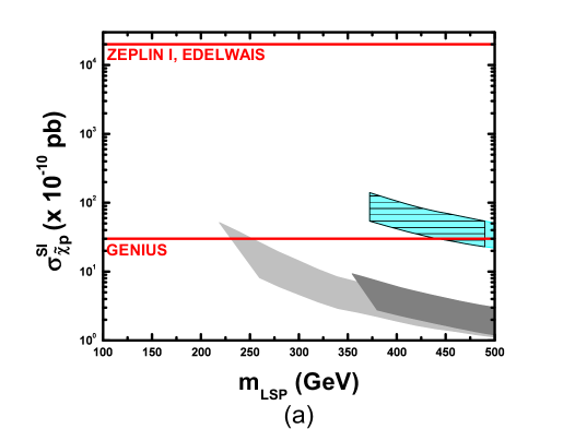
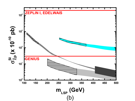
Figure 5: $\sigma_{\tilde{\chi}p}^{\rm SI}$ versus $m_{\rm LSP}$ for (a) $\Delta_{A}=0.1$ and high (light grey band, $r_{\tilde{f}}=1$) or low (grey, $r_{\tilde{f}}=1$, and cyan, $r_{\tilde{f}}=0.4$, bands) $m_{0}$ (b) $\Delta_{\tilde{b}_{2}}=0.1$ for $r_{\tilde{f}}=0.4$ (gray and cyan bands), $\Delta_{\tilde{\nu}_{\tau}}=0$ for $r_{\tilde{f}}=0.2$ (light gray band) and $\Delta_{\tilde{\tau}_{2}}=0$ for $r_{\tilde{f}}=1$ (dark gray band). Gray (light, normal and dark) shaded bands are for $r_{2}=r_{3}=1$, while cyan shaded bands are for $r_{2}=0.6,r_{3}=0.6~{}[0.5]$ (a [b]). Ruled are the areas favored by the optimistic upper bound on $m_{\rm LSP}$ from Eq. (14a), whereas the preferred region of $\sigma_{\tilde{\chi}p}^{\rm SI}$ from various projects is, also, approximately limited.

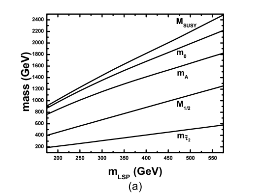
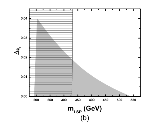
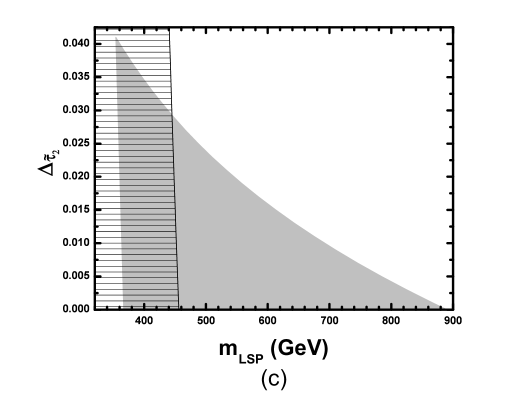
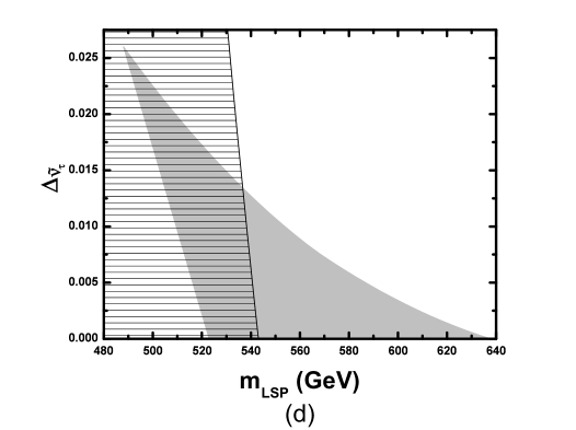
Figure 6: The mass parameters $M_{1/2}$, $m_{0}$, $m_{A}$, $M_{\rm SUSY}$ and $m_{\tilde{\tau}_{2}}$ versus $m_{\rm LSP}$ for $r_{\tilde{f}}=0.2,r_{2}=r_{3}=1$ and $\Delta_{\tilde{\nu}_{\tau}}=0$ (a) and the allowed (shaded) area for $r_{\tilde{f}}=0.2~{}[0.4],r_{2}=1~{}[0.6],r_{3}=1~{}[0.6]$ (b [d]), on the $m_{\rm LSP}-\Delta_{\tilde{\nu}_{\tau}}$ plane and for $r_{\tilde{f}}=0.4,r_{2}=0.6,r_{3}=1$ on the $m_{\rm LSP}-\Delta_{\tilde{\tau}_{2}}$ plane (c). Ruled is, also, the area favored by the optimistic upper bound on $m_{\rm LSP}$ from Eq. (14a).

5.4 $\mbox{$\tilde{\chi}$}(-\mbox{${\tilde{\chi}_{2}^{\pm}}$}-\mbox{${\tilde{\chi}_{2}^{0}}$})-\mbox{$\tilde{\nu}_{\tau}$}-\mbox{$\tilde{\tau}_{2}$}$ COANNIHILATIONS

For low enough $r_{\tilde{f}}$’s and $r_{2}=r_{3}=1$, to keep $\tilde{b}_{2}$ heavier than $\tilde{\chi}$, we must decrease the difference between the values $M_{1/2}$ and $m_{0}$ depicted in Fig. 4-(a). The increase of $M_{1/2}$ increases efficiently $m_{\tilde{Q}}$ and $m_{\tilde{b}^{c}}$ whose the running (see e.g. Ref. [66]) depends crucially on $M_{3}$ but does not affect a lot $m_{\tilde{L}}$, which is anyway low at $M_{\rm GUT}$, due to Eq. (22). Therefore, an even new type of CAM between $\mbox{$\tilde{\chi}$}-\mbox{$\tilde{\nu}_{\tau}$}-\mbox{$\tilde{\tau}_{2}$}$ emerges for $0<r_{\tilde{f}}<0.27$. Note that the sneutrino of the two first generations do not participate to this phenomenon remaining heavier, since their running does not depend on $m_{\tilde{L}}$.

We present the mass parameters, in this case, $M_{1/2}$, $m_{0}$, $m_{A}$ and $M_{\rm SUSY}$ together with $m_{\tilde{\tau}_{2}}$ versus $m_{\rm LSP}$ for $\Delta_{\tilde{\nu}_{\tau}}=0$, $r_{\tilde{f}}=0.2$ and $r_{2}=r_{3}=1$ in Fig. 6-(a). We see that $m_{\tilde{\tau}_{2}}$ is just 6% heavier than $m_{\rm LSP}$ and consequently, participates to the CAM (unlike the similar case of Ref. [23]). A typical example of the resulting allowed area on the $m_{\rm LSP}-\Delta_{\tilde{\nu}_{\tau}}$ plane is displayed in Fig. 6-(b) for the same $r_{2}$ and $r_{3}$. The left (almost vertical) [right curved] boundary of the allowed (shaded) region comes from Eq. (11b [3]). Similar is, also, the origin of the boundaries of the allowed regions for $r_{\tilde{f}}=0.4,r_{2}=0.6$ and $r_{3}=1~{}[0.6]$ presented in Fig. 6-(c [d]). There, we fix $r_{\tilde{f}}=0.4$ since for lower $r_{\tilde{f}}$, $\tilde{\nu}_{\tau}$ turns out to be lighter than $\tilde{\chi}$. Also, we take $r_{3}=0.6$, and not 0.5 as previously, since for lower $r_{3}$’s, $\tilde{b}_{2}$ becomes predominantly coannihilator. In the case of Fig. 6-(c), $m_{\tilde{\tau}_{2}}$ turns out to be slightly lighter than $m_{\tilde{\nu}_{\tau}}$ and so, the allowed area is presented on the $m_{\rm LSP}-\Delta_{\tilde{\tau}_{2}}$ plane. Also, the allowed region of Fig. 6-(d) is disconnected to this of Fig. 2-(b).

Table 3: DOMINANT CONTRIBUTIONS TO $\Omega_{\rm LSP}h^{2}$

MODEL PARAMETERS
$r_{\tilde{f}}$	$0.2$	$0.4$	$0.4$
$r_{2},r_{3}$	$r_{2}=r_{3}=1$	$r_{2}=0.6,r_{3}=1$	$r_{2}=0.6,r_{3}=0.6$
ALLOWED RANGES
$\tan\beta$	$34.2-37.7$	$34.3-36.6$	$34.8-35.5$
$m_{\rm LSP}~{}({\rm GeV})$	$201-(330)542$	$354-(456)890$	$488-(543)638$
$\Delta_{\tilde{\nu}_{\tau}}$	$0.04-0$	$0.055-0.002$	$0.026-0$
PROCESSES WHICH CONTRIBUTE MORE THAN $5\%$
PROCESS	CONTRIBUTION ($\%$)
$\mbox{$\tilde{\chi}$}\mbox{$\tilde{\chi}$}\rightarrow b\bar{b}$	$-$	$12-6$	$16-1$
$\mbox{$\tilde{\chi}$}\mbox{$\tilde{\nu}_{\tau}$}\rightarrow\tau W^{-}$	$20-6$	$7-3$	$4-4$
$\mbox{$\tilde{\chi}$}\mbox{$\tilde{\nu}_{\tau}$}\rightarrow\nu_{\tau}Z$	$11.6-0$	$-$	$-$
$\mbox{$\tilde{\chi}$}\mbox{$\tilde{\tau}_{2}$}\rightarrow\tau h$	$-$	$6-1.5$	$-$
$\mbox{$\tilde{\chi}$}\mbox{$\tilde{\tau}_{2}$}\rightarrow\nu_{\tau}W^{-}$	$-$	$7-1$	$6-4$
$\mbox{$\tilde{\chi}$}\mbox{$\tilde{\tau}_{2}$}\rightarrow\tau Z$	$-$	$6-2$	$-$
$\mbox{$\tilde{\nu}_{\tau}$}\mbox{$\tilde{\nu}_{\tau}$}\rightarrow\nu_{\tau}\nu_{\tau}$	$19-17$	$-$	$5-12$
$\mbox{$\tilde{\nu}_{\tau}$}\mbox{$\tilde{\nu}^{\ast}_{\tau}$}\rightarrow ZZ$	$10.5-12$	$-$	$3-7$
$\mbox{$\tilde{\nu}_{\tau}$}\mbox{$\tilde{\nu}^{\ast}_{\tau}$}\rightarrow W^{+}W^{-}$	$12-13.5$	$-$	$3-7$
$\mbox{$\tilde{\tau}_{2}$}\mbox{$\tilde{\nu}^{\ast}_{\tau}$}\rightarrow\nu_{\tau}\tau$	$0-9$	$-$	$-$
$\mbox{$\tilde{\tau}_{2}$}\mbox{$\tilde{\nu}^{\ast}_{\tau}$}\rightarrow\gamma W^{-}$	$2-6$	$-$	$-$
$\mbox{$\tilde{\tau}_{2}$}\mbox{$\tilde{\nu}^{\ast}_{\tau}$}\rightarrow\bar{t}b$	$-$	$-$	$2-18$
$\mbox{$\tilde{\tau}_{2}$}\mbox{$\tilde{\nu}_{\tau}$}\rightarrow\nu_{\tau}\tau$	$0.5-2.6$	$-$	$5-10$
$\mbox{$\tilde{\tau}_{2}$}\mbox{$\tilde{\tau}_{2}$}\rightarrow\tau\tau$	$0.7-6$	$5-6$	$4-10$
$\mbox{$\tilde{\tau}_{2}$}\mbox{$\tilde{\tau}^{\ast}_{2}$}\rightarrow W^{+}W^{-}$	$0.6-6$	$-$	$3-7$
$\mbox{$\tilde{\tau}_{2}$}\mbox{$\tilde{\tau}^{\ast}_{2}$}\rightarrow b\bar{b}$	$-$	$3-20$	$-$

The allowed ranges of $m_{\rm LSP}$, $\Delta_{\tilde{\nu}_{\tau}}$ and $\tan\beta$ are listed in the Table 3. For $m_{\rm LSP}$ indicated in the parenthesis, satisfaction of Eq. (14a) occurs, too. We deduce that, despite the presence of an extra coannihilator, the reduction of $\Omega_{\rm LSP}h^{2}$ caused by $\mbox{$\tilde{\chi}$}-\mbox{$\tilde{\nu}_{\tau}$}-\mbox{$\tilde{\tau}_{2}$}$ CAM is not more efficient than the case $\mbox{$\tilde{\chi}$}-\mbox{$\tilde{\tau}_{2}$}$ CAM and therefore, the maximal allowed $m_{\rm LSP}$’s do not essentially differ. However, thanks to the heavier higgs sector, Eq. (11b) is satisfied for lighter charginos and neutralinos, and consequently (see sec. 2.6), there is parameter space, where the putative bound of Eq. (14a) can be fulfilled, too. We observe, also, that although the contribution of $\mbox{$\tilde{\chi}$}-\mbox{${\tilde{\chi}_{2}^{\pm}}$}-\mbox{${\tilde{\chi}_{2}^{0}}$}$ CAM for the used $r_{2}=r_{3}\neq 1$ is very weak, it leads to a sizable suppression of $\Omega_{\rm LSP}h^{2}$ increasing the upper bound on $m_{\rm LSP}$.

The $\sigma_{\tilde{\chi}p}^{\rm SI}$ versus $m_{\rm LSP}$ for $\Delta_{\tilde{\nu}_{\tau}}=0$, $r_{\tilde{f}}=0.2$ and $r_{2}=r_{3}=1$ is depicted in Fig. 5-(b), light grey band. We observe that although the maximal $\sigma_{\tilde{\chi}p}^{\rm SI}$ lies below the range of Eq. (6), it is significantly higher than in the case with $\Delta_{\tilde{\tau}_{2}}=0$ and $r_{\tilde{f}}=r_{2}=r_{3}=1$ (dark grey band), due to the easier satisfaction of Eq. (11b). Possible diminution of $r_{2}$ and/or $r_{3}$ do not produce any improvement, since the lowest possible $m_{\rm LSP}$, derived again from Eq. (11b), increases enough (note that ${\rm BR(b\to s\gamma)}|_{\rm SUSY}$ increases lowering $m_{\tilde{\chi}^{\pm}}$).

If we had assumed UGMs with $\mu<0$ and $r_{\tilde{f}}=0.2$, the lower bound on $m_{\rm LSP}$ would have been derived from Eq. (15a) with result $m_{\rm LSP}\gtrsim 289~{}{\rm GeV}$. Consequently, a region similar to this of Fig. 6-(b) would have been allowed with maximal $\Delta_{\tilde{\nu}_{\tau}}\simeq 0.025$.

6 CONCLUSIONS-OPEN ISSUES

We considered a MSSM version which could emerge from the breakdown of a $SU(5)$ or $SO(10)$ SUSY model at GUT scale. Namely, we assumed $b-\tau$ YU, allowing gaugino and sfermion mass non-universality. We then restricted the parameter space of the model by imposing the constraints from CDM, SUSY corrections to $b$-quark mass, ${\rm BR}(b\rightarrow s\gamma)$, $\delta\alpha_{\mu}$ and accelerator data and derived scalar neutralino-proton cross sections. SUSY spectra and scalar neutralino-proton cross sections were calculated by using our numerical code, while the values of the various constraints, by employing the current version of micrOMEGAs package, supplemented by an updated ${\rm BR}(b\rightarrow s\gamma)$ code.

We showed that an opposite sign on the asymptotic gluino mass, based on group theoretical grounds, assists us to succeed compatibility between the $b-\tau$ YU and the lower bound from the $\delta\alpha_{\mu}$ constraint ($e^{+}e^{-}$-based calculation). We, then, parameterized the possible non-universality in the (i) gaugino sector, defining $r_{2},~{}r_{3}$ as the ratios between the asymptotic wino and gluino masses with the bino (ii) sfermion sector, defining $r_{\tilde{f}}$, as the ratio between the asymptotic sfermion masses in ${\bf 10}$ and ${\bf\bar{5}}$ reps of $SU(5)$ (iii) Higgs sector, defining $r_{H_{1}},~{}r_{H_{2}}$ as the ratio between the two asymptotic Higgs masses and asymptotic sfermion masses in ${\bf 10}$ reps. We used universal Higgs masses with $r_{H_{1}}=r_{H_{2}}=1$.

We found regions of the parameter space consistent with all the imposed restrictions, paying special attention to each applied $\Omega_{\rm LSP}h^{2}$ reduction “procedure”. Regarding this issue for $r_{2}=r_{3}=1$, we can distinguish the cases: (i) For $0<r_{\tilde{f}}\leq 1.2~{}[\sqrt{2}]$, $A$PE [and/or $\mbox{$\tilde{\chi}$}-\mbox{$\tilde{\tau}_{2}$}$ CAM] can drastically reduce $\Omega_{\rm LSP}h^{2}$ and succeed to bring it below the CDM upper bound for $m_{\rm LSP}$’s allowed by ${\rm BR}(b\rightarrow s\gamma)$. The LSP mass can be as low as $205~{}{\rm GeV}$ for $r_{\tilde{f}}=1$. (ii) For $0.27\leq r_{\tilde{f}}\leq 0.56$, $\mbox{$\tilde{\chi}$}-\mbox{$\tilde{b}_{2}$}$ CAM can be activated. The lowest possible LSP is $83~{}{\rm GeV}$ for $r_{\tilde{f}}=0.48$ but much heavier residual SUSY spectrum. (iii) For $0<r_{\tilde{f}}<0.27$, $\mbox{$\tilde{\chi}$}-\mbox{$\tilde{\nu}_{\tau}$}-\mbox{$\tilde{\tau}_{2}$}$ CAM can be applied. The lowest possible LSP is $174~{}{\rm GeV}$ for $r_{\tilde{f}}=0.26$ and not too heavier SUSY spectrum. In both latter cases, satisfaction of the optimistic upper bound from $\delta\alpha_{\mu}$ can be, also, achieved in sharp contrast with the universal-like case (i). Interesting scalar neutralino-proton cross section is obtained in the case of $\mbox{$\tilde{\chi}$}-\mbox{$\tilde{b}_{2}$}$ CAM due to the $\mbox{$\tilde{\chi}$}-\mbox{$\tilde{b}_{2}$}$ proximity and the light lowest $m_{\rm LSP}$. If we had imposed UGMs, we would have had qualitatively similar results, with, in general, higher $\tan\beta$’s and lowest $m_{\rm LSP}$’s but with restrictions on the parameters, derived from the $\tau$-based calculation of $\alpha^{\rm SM}_{\mu}$.

In our investigation, we considered, also, cases for $r_{2}=0.6$ and/or $r_{3}=1,0.6,0.5$. In these, gaugino inspired CAMs ($\mbox{$\tilde{\chi}$}-\mbox{${\tilde{\chi}_{2}^{\pm}}$}-\mbox{${\tilde{\chi}_{2}^{0}}$}$) can be activated and combined with the former sfermionic CAMs, creating new, privileged situations in the $\Omega_{\rm LSP}h^{2}$ calculation without to reduce it far lower than the expectations. In most cases the lowest and the highest possible $m_{\rm LSP}$’s are higher than the former cases. Consequently, no important improvement on the maximal scalar neutralino-proton cross section is observed, although the gaugino purity of LSP is decreased.

Lastly, we should discuss the fate of the sfermionic CAMs in the predictive cases in which the arrangement of Eq. (19) is “spontaneously” produced. Namely with dominance of (i) 24 reps in Eq. (20) for the case of $SU(5)$, we take [58] $r_{2}=3$ and $r_{3}=2$. We observe that both new sfermionic CAMs can be activated for lower $r_{\tilde{f}}$ ’s. (ii) 54 reps in Eq. (20) for the case of $SO(10)$, and for the symmetry breaking pattern $SO(10)\to SU(4)_{\rm c}\otimes SU(2)_{L}\otimes SU(2)_{R}$, we take [65] $r_{2}=3/2$ and $r_{3}=1$ with results quite similar to those with $r_{2}=r_{3}=1$ (iii) 54 reps in Eq. (20) for the case of $SO(10)$ and for the symmetry breaking pattern $SO(10)\to SU(2)\otimes SO(7)$, we take $r_{2}=-7/3$ and $r_{3}=-1$. $\mbox{$\tilde{\chi}$}-\mbox{$\tilde{b}_{2}$}$ CAM is similarly achieved but $\mbox{$\tilde{\chi}$}-\mbox{$\tilde{\nu}_{\tau}$}-\mbox{$\tilde{\tau}_{2}$}$ CAM can not occur.

Our results do not crucially dependent on our choice $r_{H_{1}}=r_{H_{2}}=1$. We checked that if we had imposed $r_{H_{1}}=r_{H_{2}}=r_{\tilde{f}}$, we would have obtained similar sfermionic CAMs but for much lower $r_{\tilde{f}}$ ’s than those used here. The situation with $r_{H_{1}}\neq r_{H_{2}}$ requires certainly deeper investigation, since, then, additional contributions in the RGEs arise [23] and much more rich situations can emerge.

For simplicity, $m^{\rm c}_{b}(M_{Z})$ was fixed to its central experimental value throughout our calculation. Allowing it to vary within its $95\%$ c.l. range of Eq. (9), the allowed ranges of $\tan\beta$ will further widen. At least, the non-universality in the gaugino sector can cause, through $c_{i}$ of Eq. (20), interesting consequences to the GUT structure of the theory, such as to the proton stability (see, e.g. Refs. [75, 60, 76]). However, such an analysis is outside the scope of this work.