The total cross section for Higgs production in bottom-quark annihilation is evaluated at next-to-next-to-leading order in QCD. This is the first time that all terms at order $\alpha_{s}^{2}$ are taken into account. We find a greatly reduced scale dependence with respect to lower order results, for both the factorization and the renormalization scales. The behavior of the result is consistent with earlier determinations of the appropriate factorization scale for this process of $\mu_{F}\approx M_{H}/4$, and supports the validity of the bottom parton density approach for computing the total inclusive rate. We present precise predictions for the cross section at the Fermilab Tevatron and the CERN Large Hadron Collider.

Higgs boson production in bottom quark fusion at next-to-next-to-leading order

I Introduction

The search for the Higgs boson will be a top priority of the CERN Large Hadron Collider (LHC). The LHC’s discovery potential for the Standard Model Higgs boson fully covers the mass range from the experimental lower bound established by the LEP experiments ($M_{H}\gtrsim 114$ GeV) up to $M_{H}\approx 1$ TeV, beyond which the concept of the Higgs boson as an elementary particle becomes questionable. In addition, the Fermilab Tevatron could find evidence for or even discover the Higgs boson if $M_{H}\lesssim 180$ GeV and if sufficient luminosity lumimoni can be collected.

The theoretical description of the signal processes for Standard Model Higgs boson production is under good control. For a review, see Ref. Carena:2002es . The dominant production mode is gluon fusion, for which the next-to-next-to-leading order (NNLO) corrections are now available Harlander:2002wh ; Anastasiou:2002yz and have recently been reconfirmed by Ref. Ravindran:2003um . The radiative corrections for the weak boson fusion channel Han:1992hr and associated production with a weak gauge boson Han:1991ia have been known for several years, rendering the theoretical uncertainty in these processes very small. Recently, next-to-leading order (NLO) corrections have also been evaluated for Higgs boson production in association with top quarks Reina:2001sf ; Beenakker:2001rj ; Dawson:2002tg ; Beenakker:2002nc , resulting in a drastic reduction of the scale uncertainty.

These results can be used for supersymmetric Higgs boson production as well. However, because of the enriched particle spectrum in supersymmetric extensions of the Standard Model, they provide only a part of the full production rate in general. Additional contributions arise through intermediate supersymmetric partners Dawson:1996xz and modified couplings of the Standard Model particles. In order to avoid unnecessary generalizations, we will focus on the Minimal Supersymmetric Standard Model (MSSM) for the rest of this paper (see, e.g., Ref. Martin:1997ns for an outline of the MSSM). The extent to which our results can be transferred to other models should be clear from this discussion.

The MSSM contains two Higgs doublets, one giving mass to up-type quarks and the other to down-type quarks. The associated vacuum expectation values are labeled $v_{u}$ and $v_{d}$, respectively, and they determine the MSSM parameter $\tan\beta\equiv v_{u}/v_{d}$. After spontaneous symmetry breaking, there are five physical Higgs bosons, whose mass eigenstates are denoted by $h$ (“light scalar”), $H$ (“heavy scalar”), $H^{\pm}$ (“charged scalars”), and $A$ (“pseudoscalar”). One interesting consequence of this more complicated Higgs sector is that, compared to the Standard Model, the bottom quark Yukawa coupling can be enhanced with respect to the top quark Yukawa coupling. In the Standard Model, the ratio of the $t\bar{t}H$ and $b\bar{b}H$ couplings is given at the tree-level by $\lambda^{\rm SM}_{t}/\lambda^{\rm SM}_{b}=m_{t}/m_{b}\approx 35$. In contrast, in the MSSM, it depends on the value of $\tan\beta$. At leading order,

$$\frac{\lambda^{{\rm\small MSSM}}_{t}}{\lambda^{{\rm\small MSSM}}_{b}}=f_{\phi}(\alpha)\,\frac{1}{\tan\beta}\cdot\frac{m_{t}}{m_{b}}\,,$$ (1)

with

$$f_{\phi}(\alpha)=\left\{\begin{array}[]{ll}-\cot\alpha\,,&\qquad\phi=h\,,\\ \phantom{-}\tan\alpha\,,&\qquad\phi=H\,,\\ \phantom{-}\cot\beta\,,&\qquad\phi=A\,,\end{array}\right.$$

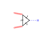
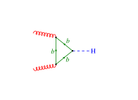
(a)	(b)

Figure 1: For large $\tan\beta$, the bottom quark contribution to the gluon fusion process can be comparable to the top quark contribution.

where $\alpha$ is the mixing angle between the weak and the mass eigenstates of the neutral scalars. A value of $\tan\beta$ as large as $30-40$ could be accommodated fairly naturally in the MSSM. Such an enhancement would have (at least) two important consequences. The first is that in the gluon fusion mode it is no longer sufficient to consider top quark loops as the only mediators between the Higgs boson and the gluons; one must also include the effects of bottom quark loops (see Fig. 1). Since one cannot justify the use of an effective field theory in which the bottom quarks are integrated out, this involves computing massive multi-loop diagrams. While the massive NLO calculation (including massive two-loop virtual diagrams) was performed some time ago Spira:1995rr , the NNLO result (requiring up to three loops for the virtual correction) is still beyond the limits of current calculational technology.

The second consequence is that Higgs boson production in association with bottom quarks can become an important channel: $p\tilde{p}\to b\bar{b}\phi$ ($\tilde{p}\in\{p,\bar{p}\}$ and $\phi\in\{h,H,A\}$ here and in what follows). At first sight, the evaluation of the corresponding cross section is in close analogy to the process $p\tilde{p}\to t\bar{t}\phi$. But this is only true if the bottom quarks are observed in the detector, and are thus restricted to large transverse momenta. If at least one of the bottom quarks escapes detection, the production rate must be integrated over all transverse momenta of this bottom quark. Since the Higgs boson is much heavier than the bottom quark, this integration leads to collinear logarithms, $\ln(m_{b}/M_{\phi})$, which require a more careful analysis than in the case of $t\bar{t}\phi$ production.

The subject of this paper is the precise prediction of the total cross section for Higgs boson production in association with bottom quarks, where neither bottom quark need be detected. This requires integrating over the transverse momenta of both final state bottom quarks. Each integration gives rise to collinear logarithms of the kind mentioned above. Since the bottom quarks may remain undetected, it is more appropriate to view our result as a part of the total inclusive Higgs production rate $\sigma(p\tilde{p}\to\phi+X)$. In order to emphasize this point, we shall henceforth denote the fully inclusive process mediated through bottom–antibottom annihilation as $p\tilde{p}\to(b\bar{b})\phi+X$.

Our calculation is based on the approach of Refs. Dicus:1989cx ; Dicus:1998hs ; Maltoni:2003pn , where the leading-order (LO) partonic process is taken to be $b\bar{b}\to\phi$. We will refer to this as the variable flavor number scheme (VFS) approach in what follows, as opposed to the fixed flavor number scheme (FFS) approach, where the tree-level process $gg\to b\bar{b}\phi$ is taken as the lowest-order contribution and bottom quarks cannot appear in the initial state. The initial state bottom quarks in the VFS approach arise (predominantly) from gluon splitting in the proton, parametrized in terms of bottom quark parton distributions Barnett:1988jw ; Olness:1988ep ; Aivazis:1994pi ; Thorne:1998ga ; Kramer:2000hn ; Buza:1996ie ; Buza:1998wv ; Chuvakin:1999nx ; Chuvakin:2000qc ; Chuvakin:2000jm ; Chuvakin:2000zj . In this way, the large collinear logarithms that arise due to the fact that the colliding gluons carry a momentum of the order of $M_{\phi}/2\gg m_{b}$ can be resummed through DGLAP evolution. The convolution of these bottom quark densities with the partonic cross section leads to the hadronic cross section $\sigma\left[p\tilde{p}\to(b\bar{b})\phi+X\right]$.

This process has been a subject of interest for some time. It is currently known up to NLO in the VFS approach Eichten:1984eu ; Gunion:1987pe ; Olness:1988ep ; Dicus:1989cx ; Dicus:1998hs ; Maltoni:2003pn . In the FFS approach, the calculation is analogous to $t\bar{t}\phi$ production, which is also known to NLO Raitio:1979pt ; Ng:1984jm ; Kunszt:1984ri ; Reina:2001sf ; Beenakker:2001rj ; Dawson:2002tg ; Beenakker:2002nc . The case where one bottom quark is tagged has been computed at NLO in Ref. Campbell:2002zm ; in that case, the LO process in the VFS approach is $bg\to b\phi$.

There has been an ongoing discussion as to the relative merits of the VFS and FFS approaches Dicus:1998hs ; Balazs:1998sb ; Campbell:2002zm ; Maltoni:2003pn ; Rainwater:2002hm ; Spira:2002rd , especially because the results of the two approaches disagree by more than an order of magnitude for the scale choice $\mu_{F}=\mu_{R}=M_{\phi}$, where $\mu_{F}$ and $\mu_{R}$ are the factorization and the renormalization scales, respectively. Recently, it has been argued Maltoni:2003pn , that the proper factorization scale for this process should be $\mu_{F}\approx M_{\phi}/4$ instead of $M_{\phi}$. Indeed, for this choice, the disagreement between the VFS and the FFS approach is significantly reduced. The result of our paper demonstrates the self-consistency of the VFS approach and confirms the proposed factorization scale of Ref. Maltoni:2003pn as the appropriate choice.

Given the considerations above, the motivations for a NNLO calculation are manyfold. One is to examine the assertion that $\mu_{F}\approx M_{\phi}/4$ is the proper choice for this process at NLO Plehn:2002vy ; Maltoni:2003pn . If the higher order corrections are minimal at that scale, this would be a strong argument in favor of the validity of the VFS approach to $(b\bar{b})\phi$ production. A second motivation, as will be discussed in more detail below, is that the NNLO terms play an exceptional role in the VFS approach to $(b\bar{b})\phi$ production due to the fact that they are the first to consistently include the “parent” process, $gg\to b\bar{b}\phi$, and thereby sample the same range of bottom quark transverse momenta as the LO FFS approach. A third and perhaps dominant motivation for the NNLO calculation is to reduce the sensitivity of the calculation to the unphysical scale parameters $\mu_{F}$ and $\mu_{R}$, thereby removing a significant source of uncertainty from the theoretical prediction.

In this paper we will present results for the process $p\tilde{p}\to(b\bar{b})\phi+X$ at NNLO. As will be shown, they nicely meet all expectations concerning their dependence on the renormalization and factorization scales, thus providing a solid prediction for the total cross section at the LHC and the Tevatron. The inclusive production cross section could have phenomenological implications for the observation of the supersymmetric $H$ and $A$ bosons, for example, in the $H/A\to\mu^{+}\mu^{-}$ decay mode.

The organization of the paper is as follows: In Sec. II we discuss the VFS approach to computing the $p\tilde{p}\to(b\bar{b})\phi+X$ process and its motivations. In Sec. III we describe the actual calculation and in Sec. IV we present our numerical results. Analytic results for the partonic cross sections are presented in the appendix.

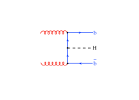
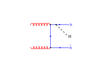
(a)	(b)
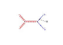
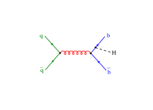
(c)	(d)

Figure 2: Partonic processes for $pp\to b\bar{b}H$. Not shown are diagrams that can be obtained by crossing the initial state gluons, or radiating the Higgs off an antibottom quark.

II Theoretical description of the production rate

In the FFS approach, the LO partonic process for the production of a Higgs boson in association with a bottom quark pair is of order $\alpha_{s}^{2}$. A few typical diagrams are shown in Fig. 2. Because of the large mass difference between the bottom quark and the Higgs boson, the total cross section contains large logarithms of the form

$$\begin{split}l_{b}\equiv\ln(m_{b}^{2}/\mu_{\phi}^{2})\,,\end{split}$$ (2)

where $\mu_{\phi}$ is of the order of $M_{\phi}$. More precisely, every on-shell gluon that splits into a $b\bar{b}$ pair with an on-shell bottom quark generates one power of that logarithm. Thus, Figs. 2(a) and 2(b) generate two and one power of $l_{b}$, respectively, while Figs. 2(c) and 2(d) do not generate any $l_{b}$ terms. Furthermore, each higher order in perturbation theory brings in another power of $l_{b}$ due to the radiation of gluons from bottom quarks.

Because $l_{b}\sim\ln(m_{b}^{2}/M_{\phi}^{2})$ is rather large, $\alpha_{s}l_{b}$ is not a good expansion parameter. It would be better to re-organize the perturbative series such that terms like $(\alpha_{s}l_{b})^{n}$ are resummed to all orders in $n$. This resummation can be achieved by introducing bottom quark parton distribution functions which contain all the collinear terms arising from the splitting of gluons into $b\bar{b}$ pairs Barnett:1988jw ; Olness:1988ep ; Aivazis:1994pi ; Thorne:1998ga ; Kramer:2000hn ; Buza:1996ie ; Buza:1998wv ; Chuvakin:1999nx ; Chuvakin:2000qc ; Chuvakin:2000jm ; Chuvakin:2000zj . This constitutes the motivation for using the VFS approach.

Convolving the tree-level process of Fig. 3(a) with these bottom quark distributions will resum the leading logarithms of the form $(\alpha_{s}l_{b})^{2}\cdot(\alpha_{s}l_{b})^{n}$, $n\geq 0$. In order to retain subleading logarithms, one has to compute higher orders. For example, including the NLO contributions with all the relevant subprocesses ($b\bar{b}\to h$, $b\bar{b}\to hg$, $gb\to hb$, and $g\bar{b}\to h\bar{b}$), resums the terms of order $\alpha_{s}^{2}l_{b}\,(\alpha_{s}l_{b})^{n}$, $n\geq 0$. In order to retain all powers of $l_{b}$ at order $\alpha_{s}^{2}\,\sum_{n}(\alpha_{s}l_{b})^{n}$, it is necessary to evaluate the cross section up to NNLO.

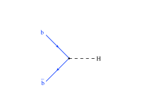
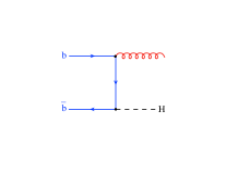
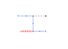
(a)	(b)	(c)

Figure 3: Lowest order diagrams contributing to (a) $b\bar{b}\to H$, (b) $b\bar{b}\to Hg$, and (c) $bg\to Hb$. At NNLO, these diagrams receive corrections up to two loops in case (a), and one loop in case (b) and (c).

Let us briefly review the idea of the VFS in its simplest form. Assume $n_{\ell}=n_{f}-1$ massless quark flavors and one massive quark flavor of mass $m_{h}$. First, one defines parton densities $f^{(n_{\ell})}_{i}(x,Q^{2})$ for the gluon ($i=g$) and the massless flavors ($i=1,\ldots,n_{\ell}$) in the standard way, obeying DGLAP evolution with $n_{\ell}$ active flavors. The heavy quark density $f^{(n_{\ell})}_{n_{f}}(x,Q^{2})$ is assumed to vanish. Partonic processes involving the heavy quark should be evaluated by keeping the heavy quark mass. This is called the $n_{\ell}$-flavor scheme.

At a certain scale $\mu_{h}^{2}$, one relates the $n_{\ell}$- to the $n_{f}$-flavor scheme by defining initial conditions for new parton densities $f^{(n_{f})}_{i}$ in terms of the $f^{(n_{\ell})}_{i}$:

$$\begin{split}f^{(n_{f})}_{i}(x,Q^{2}=\mu_{h}^{2})&=\sum_{j}C_{ij}(\mu_{h}/m_{h})\otimes f^{(n_{\ell})}_{j}(x,Q^{2}=\mu_{h}^{2})\,,\\ i&=g,1,\ldots,n_{f}\qquad j=g,1,\ldots,n_{\ell}\,.\end{split}$$ (3)

The $C_{ij}$ are determined by the requirement that physical quantities are the same (up to higher orders in $\alpha_{s}$) in both the $n_{\ell}$- and the $n_{f}$-flavor scheme. (This requirement may be implemented asymptotically or using mass dependent terms Aivazis:1994pi ; Thorne:1998ga ; Buza:1998wv ; Chuvakin:1999nx .) Above the matching scale, the DGLAP evolution of the $f^{(n_{f})}_{i}(x,Q^{2})$ ($i=g,1,\ldots,n_{f}$) is performed with $n_{f}$ active flavors.

In general, one assumes the $n_{\ell}$-flavor scheme at scales $Q^{2}\lesssim m_{h}^{2}$ and switches to the $n_{f}$-flavor scheme at larger values of $Q^{2}$. It is also convenient to choose the matching scale in Eq. (3) as $\mu_{h}^{2}=m_{h}^{2}$, which avoids the occurrence of logarithms of $m_{h}/\mu_{h}$.

For our purposes, $m_{h}^{2}/Q^{2}\sim m_{b}^{2}/M_{\phi}^{2}\lesssim 0.003$, so threshold effects from the matching prescription should be minimal. For the same reason, it is justified to neglect the bottom quark mass in the partonic process (apart from Yukawa couplings, of course). Indeed, masses must be neglected for initial state bottom quarks in order to avoid violation of the Bloch-Nordsieck theorem (and the consequent failure to fully cancel infrared divergences) at NNLO and beyond Catani:1988xy .

In order to make the following discussion more transparent, let us write the fully inclusive $(b\bar{b})\phi$ production rate in the VFS approach schematically as follows:

$$\begin{split}\sigma(p\tilde{p}\to&(b\bar{b})\phi+X)=\\ &\sum_{n=0}^{\infty}\left(\alpha_{s}l_{b}\right)^{n}\bigg{\{}\alpha_{s}^{2}\,\left[c_{n0}\,l_{b}^{2}+c_{n1}\,l_{b}+c_{n2}\right]\\ &\qquad+\alpha_{s}^{3}\,d_{n3}+\alpha_{s}^{4}\,d_{n4}+\alpha_{s}^{5}\,d_{n5}+\cdots\bigg{\}}\,.\end{split}$$ (4)

The sum over $n$ is implicit in the parton densities. A LO calculation determines the coefficients $c_{n0}$, while NLO adds the coefficients $c_{n1}$. Note that the subprocess $bg\to b\phi$ does not fully determine the coefficients $c_{n1}$; in order to obtain the correct resummation at $\alpha_{s}^{n}l_{b}^{n-1}$ ($n\geq 2$), one has to include the real and virtual corrections to the $b\bar{b}\to\phi$ subprocess as well. In the same way, the sum of all subprocesses that contribute at second order determines $c_{n2}$ ($n\geq 0$), and thus all terms associated with the order $\alpha_{s}^{2}\,(\alpha_{s}l_{b})^{n}$. The NNLO result is thus the first to include all terms of order $\alpha_{s}^{2}$ (as well as higher order terms resummed in the parton distribution functions). Higher orders in perturbation theory correspond to the coefficients $d_{nk}$; their $l_{b}$ terms are — formally — completely contained in the parton densities. This illustrates once more the exceptional role of the NNLO corrections in this approach.

The leading order terms were evaluated by Eichten et al. Eichten:1984eu . The leading $bg$ and $gg$ initiated processes (Figs. 3(c) and 2(a)) were subsequently added by Dicus and Willenbrock Dicus:1989cx . Ten years later, Dicus et al. Dicus:1998hs (see also Ref. Balazs:1998sb ) computed the full NLO contribution to $b\bar{b}\to\phi$ (and related subprocesses), which leads to the single logarithmically suppressed term $c_{n1}$ for all $n\geq 0$. Setting the renormalization and the factorization scale equal to $M_{\phi}$ ($\mu_{R}=\mu_{F}=M_{\phi}$), they found that the ${\cal O}(\alpha_{s})$-corrections to the $b\bar{b}\to\phi$ subprocess and the contribution from the tree level $bg\to\phi b$ subprocess are quite large, but of opposite sign. This leads to large cancellations which are particularly drastic at the LHC. They also observed that the contribution from $bg\to\phi b$ becomes especially large at Higgs boson masses below $\approx 150$ GeV, meaning that logarithmically suppressed terms become important in this region.

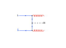
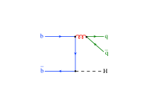
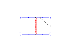
(a)	(b)	(c)
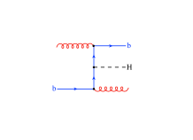
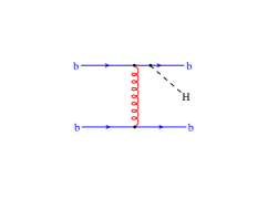
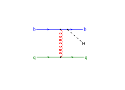
(d)	(e)	(f)

Figure 4: Diagrams contributing at NNLO. Note that the Higgs boson can couple to the $b$–quarks at any point; only representative diagrams are shown.

Recently, Maltoni et al. Maltoni:2003pn revisited the NLO calculation in the light of Ref. Plehn:2002vy , which gives an argument for the proper choice of the factorization scale when using the bottom quark density approach. Following that argument, they determined the factorization scale for the $(b\bar{b})\phi$ process to be $\mu_{F}\approx M_{\phi}/4$. With this choice, both the NLO corrections from the $gb$ and the $b\bar{b}$ initiated process turn out to be very well behaved.

As we will show in Sect. IV, the behavior of the NNLO corrections confirms this choice of scale at NLO, in the sense that the perturbation theory up to NNLO is very well behaved for this choice. This supports the method of Refs. Plehn:2002vy ; Maltoni:2003pn (see also Ref. Boos:2003yi ) for determining the factorization scale in the VFS approach at lower orders. For the process under consideration, it turns out that the dependence on the unphysical scales of the NNLO result is so weak that the discussion on the proper scale choice becomes irrelevant. The overall conclusion is that the prediction for Higgs boson production in bottom quark fusion is now under very good control.

III Outline of the calculation

As discussed before, we will neglect the bottom quark mass everywhere except in the Yukawa couplings. The calculation is thus completely analogous to, say, Drell-Yan production of virtual photons Hamberg:1991np ; Harlander:2002wh : One evaluates virtual and real corrections to Higgs production in $b\bar{b}$, $gb$, $gg$, $bb$, $qb$ and $q\bar{q}$ scattering (and the charge conjugated processes) and then performs ultraviolet renormalization and mass factorization.

The subprocesses to be evaluated at the partonic level are given as follows ($q\in\{u,d,c,s\}$):
$\bullet$ up to two loops: $b\bar{b}\to\phi$  [Fig. 3(a)] $\bullet$ up to one loop: $b\bar{b}\to\phi g$, $gb\to\phi b$  [Figs. 3(b), 3(c)] $\bullet$ at tree level: $b\bar{b}\to\phi gg$,  $b\bar{b}\to\phi q\bar{q}$, $b\bar{b}\to\phi b\bar{b}$, $gb\to\phi gb$, $bb\to\phi bb$, $bq\to\phi bq$ [Figs. 4(a)–4(f)] $gg\to\phi b\bar{b}$ [Figs. 2(a)–2(c)], $q\bar{q}\to\phi b\bar{b}$ [Fig. 2(d)] We compute the two-loop virtual terms by employing the method of Refs. Baikov:2000jg ; Harlander:2000mg , which maps them onto three-loop two-point functions. In this way, they can be reduced to a single master integral, using the reduction formulas given in Refs. Chetyrkin:1981qh ; Larin:1991fz . The master integral has been computed in Ref. Gonsalves:1983nq . The pole parts of this “$b\bar{b}\phi$ form factor” can be compared to the general formula of Refs. Catani:1998bh ; Sterman:2002qn which provides a welcome check. For the generation of the diagrams we use QGRAF Nogueira:1993ex as embedded in the automated system GEFICOM Geficom ; Steinhauser:2002rq (see also Ref. Harlander:1998dq ).

The one-loop single emission processes are obtained by computing analytically the full one-loop amplitudes, which are then interfered with the amplitudes of the tree-level processes. The two-particle phase space integrals are also computed analytically.

For the tree-level double emission processes, we express the matrix elements and phase space measures in terms of the variable $x=M_{\phi}^{2}/\hat{s}$, where $\hat{s}$ is the center of mass energy. Then we expand the integrands in terms of $(1-x)$ Harlander:2002wh . This leaves us with only one nontrivial phase space integral, independent of the order of the expansion. The regular integrands and the finite integration region ensure the validity of the interchange of integration and expansion. Keeping of the order of ten terms in the expansion in $(1-x)$ leads to a hadronic result that is already phenomenologically equivalent to the analytic result. By evaluating the expansion up to sufficiently high orders, however, one can invert the series Kilgore:2002sk by mapping the expansion onto a set of basis functions. The latter can be deduced from the known NNLO Drell-Yan result Hamberg:1991np ; Harlander:2002wh .

All algebraic manipulations are performed with the help of the program FORM Vermaseren:2000nd .

For a consistent treatment of the NNLO process, it is not sufficient to evaluate only the partonic cross section at NNLO. Another ingredient is the proper parton densities, obeying NNLO Dokshitzer-Gribov-Lipatov-Altarelli-Parisi (DGLAP) evolution. At present, only approximate evolution kernels are known, derived from moments of the structure functions Retey:2000nq ; Larin:1994vu ; Larin:1997wd . On this basis, approximate NNLO parton distribution sets have been evaluated Martin:2002dr . We use this set in all of our numerical analyses below. Once parton distributions that use exact NNLO evolution become available, it is a straightforward task to update the analysis using the partonic results presented in Appendix A.

Let us now turn to the underlying interaction and the renormalization of the partonic results. We ignore the bottom quark mass and the electroweak interactions, so for our purposes, the Lagrangian is:

$$\begin{split}{\cal L}_{b\bar{b}\phi}&=-\frac{1}{4}F^{a}_{\mu\nu}F^{a\,\mu\nu}+\sum_{q}\bar{q}\,i\kern 1.77846pt\lower 0.6458pt\hbox{/}\kern 1.77846pt\kern-8.55695pt\hbox{$D$}q+\bar{b}\,i\kern 1.77846pt\lower 0.6458pt\hbox{/}\kern 1.77846pt\kern-8.55695pt\hbox{$D$}b-\lambda_{b}^{\rm B}\bar{b}\phi{}b\,,\end{split}$$ (5)

where $F^{a}_{\mu\nu}$ is the gluon field strength tensor, $D_{\mu}$ is the QCD covariant derivative, and the sum runs over the quarks $u,d,s,c$. $\lambda_{b}^{\rm B}$ is a bare bottom Yukawa coupling constant. In the modified minimal subtraction $\left(\overline{\mbox{\small MS}}\right)$ scheme, the scalar coupling is renormalized such that

$$\begin{split}\lambda_{b}^{\rm B}&\equiv\lambda_{b}\,Z_{m}(\alpha_{s})\,,\hskip 56.9055pt\left[\phi=h,H\right]\\ Z_{m}(\alpha_{s})&=1-\frac{\alpha_{s}}{\pi}\frac{1}{\epsilon}\\ +&\left(\frac{\alpha_{s}}{\pi}\right)^{2}\,\bigg{[}\frac{1}{\epsilon^{2}}\left(\frac{15}{8}-\frac{n_{f}}{12}\right)+\frac{1}{\epsilon}\left(-\frac{101}{48}+\frac{5}{72}\,n_{f}\right)\bigg{]}\\ &+{\cal O}(\alpha_{s}^{3})\,,\end{split}$$ (6)

where $\epsilon=(4-D)/2$ and $D$ is the number of space-time dimensions in which we evaluate the loop (and phase-space) integrals. $Z_{m}(\alpha_{s})$ is identical to the quark mass renormalization constant of QCD Chetyrkin:1997dh ; Vermaseren:1997fq . Here and in the following, we use the short hand notations $\lambda_{b}\equiv\lambda_{b}^{(n_{f})}(\mu_{R})$ and $\alpha_{s}\equiv\alpha_{s}^{(n_{f})}(\mu_{R})$ for the $\overline{\mbox{\small MS}}$-renormalized Yukawa and strong coupling constants, respectively. $\mu_{R}$ is the renormalization scale, and $n_{f}$ is the number of “active” quark flavors. We will set $n_{f}=5$ in our numerical analyses.

There are (at least) two methods of obtaining the result for pseudoscalar production. The first is to replace the Yukawa interaction term in Eq. (5) with a pseudoscalar interaction,

$$\lambda_{b}^{\rm B}\bar{b}\phi{}b\longrightarrow i\lambda_{b}^{\rm B}\bar{b}\phi\gamma_{5}{}b\,,$$ (7)

and proceed by direct calculation.

The second method is to exploit the chiral symmetry of the bottom quarks in Eq. (5), which implies that we are free to perform independent left-handed and right-handed phase rotations of the bottom quarks. If we perform the rotation

$$b_{R}\to i\,b^{\prime}_{R}\hskip 85.35826ptb_{L}\to b^{\prime}_{L}\,,$$ (8)

the Lagrangian becomes

$$\begin{split}{\cal L}_{b\bar{b}\phi}\to&-\frac{1}{4}F^{a}_{\mu\nu}F^{a\,\mu\nu}+\sum_{q}\bar{q}\,i\kern 1.77846pt\lower 0.6458pt\hbox{/}\kern 1.77846pt\kern-8.55695pt\hbox{$D$}q+\bar{b}^{\prime}\,i\kern 1.77846pt\lower 0.6458pt\hbox{/}\kern 1.77846pt\kern-8.55695pt\hbox{$D$}b^{\prime}-i\lambda_{b}^{\rm B}\bar{b}^{\prime}\phi\gamma_{5}{}b^{\prime}\,,\end{split}$$ (9)

and we find the same interaction Lagrangian as in Eq. (7). This implies that the cross section for pseudoscalar Higgs boson production, written in terms of the Yukawa coupling $\lambda_{b}$, is identical to the cross section for scalar Higgs boson production to all orders in $\alpha_{s}$.

Following the prescription of Larin Larin:1993tq for the treatment of $\gamma_{5}$ in dimensional regularization, we have performed the direct calculation through NNLO and find that this is indeed the case.

Even in the direct calculation, one can see that this identity will hold to all orders in $\alpha_{s}$ with the following argument. If we square the amplitude before computing loop integrals, all fermion lines are closed loops. The fact that we set the bottom quark mass to zero means that both Higgs boson vertices (in both the scalar and pseudoscalar cases) must appear on the same fermion line. If only one Higgs vertex were to appear on a fermion line, there would be an odd number of $\gamma$ matrices in the fermion trace which would therefore vanish. In the pseudoscalar case, this means that nonvanishing fermion traces must contain either zero or two $\gamma_{5}$ matrices. The prescription of Larin Larin:1993tq allows one to assume anticommutativity of $\gamma_{5}$ and identify $\gamma_{5}^{2}=1$ when two $\gamma_{5}$-matrices are on the same fermion line. Thus, the $\gamma_{5}$-matrices can be eliminated and we see that the calculation for pseudoscalar Higgs boson production is identical, diagram by diagram of the squared amplitude, to that for scalar Higgs boson production, apart from the different Yukawa couplings.

For the sake of completeness, let us remark that the Standard Model value for the coupling constant is given by $\lambda_{b}=\sqrt{2}m_{b}/v$, where $v\approx 246$ GeV is the vacuum expectation value for the Higgs boson field, and $m_{b}$ is the running $\overline{\mbox{\small MS}}$ mass of the bottom quark, $m_{b}(\mu_{R})$, evaluated at the renormalization scale $\mu_{R}$. In the MSSM we have

$$\begin{split}\lambda_{b}&=\left\{\begin{array}[]{ll}\displaystyle-\sqrt{2}\frac{m_{b}}{v}\frac{\sin\alpha}{\cos\beta}\,,&\hskip 56.9055pt\phi=h\,,\\[15.0pt] \displaystyle\phantom{-}\sqrt{2}\frac{m_{b}}{v}\frac{\cos\alpha}{\cos\beta}\,,&\hskip 56.9055pt\phi=H\,,\\[15.0pt] \displaystyle\phantom{-}\sqrt{2}\frac{m_{b}}{v}\tan\beta\,,&\hskip 56.9055pt\phi=A\,.\end{array}\right.\end{split}$$ (10)

The renormalized partonic results have a dependence on the unphysical scales $\mu_{F}$ and $\mu_{R}$, both explicitly in terms of logarithms, and implicitly through the parameters $\alpha_{s}(\mu_{R})$ and $\lambda_{b}(\mu_{R})$. The variation of $\alpha_{s}$ and $\lambda_{b}$ with $\mu_{R}$ is governed by the renormalization group equations (RGEs)

$$\mu_{R}^{2}\frac{{\rm d}}{{\rm d}\mu_{R}^{2}}a_{s}=\beta(a_{s})\,a_{s}\,,\quad\mu_{R}^{2}\frac{{\rm d}}{{\rm d}\mu_{R}^{2}}\lambda_{b}=\gamma^{m}(a_{s})\,\lambda_{b}\,,\quad a_{s}\equiv\frac{\alpha_{s}}{\pi}\,,$$ (11)

where

$$\begin{split}\beta(a_{s})&=-a_{s}\beta_{0}-a_{s}^{2}\beta_{1}-a_{s}^{3}\beta_{2}+{\cal O}(a_{s}^{4})\,,\\[7.5pt] \beta_{0}&=\frac{11}{4}-\frac{1}{6}\,n_{f}\,,\\[7.5pt] \beta_{1}&=\frac{51}{8}-\frac{19}{24}\,n_{f}\,,\\[7.5pt] \beta_{2}&=\frac{2857}{128}-\frac{5033}{1152}\,n_{f}+\frac{325}{3456}\,n_{f}^{2}\,,\\[15.0pt] \gamma^{m}(a_{s})&=-a_{s}\gamma^{m}_{0}-a_{s}^{2}\gamma^{m}_{1}-a_{s}^{3}\gamma^{m}_{2}+{\cal O}(a_{s}^{4})\,,\\[7.5pt] \gamma^{m}_{0}&=1\,,\\[7.5pt] \gamma^{m}_{1}&=\frac{101}{24}-\frac{5}{36}\,n_{f}\,,\\[7.5pt] \gamma^{m}_{2}&=\frac{1249}{64}-\left(\frac{277}{216}+\frac{5}{6}\,\zeta_{3}\right)\,n_{f}-\frac{35}{1296}\,n_{f}^{2}\,.\end{split}$$ (12)

Here, $\zeta_{n}\equiv\zeta(n)$ is Riemann’s $\zeta$-function ($\zeta_{3}\approx 1.20206$). In order to evaluate $\alpha_{s}(\mu_{R})$ from the initial value $\alpha_{s}(M_{Z})$, $\beta(a_{s})$ is expanded up to $\alpha_{s}^{\ell}$, with $\ell=1$ at LO, $\ell=2$ at NLO, and $\ell=3$ at NNLO. The resulting differential equation of Eq. (11) is solved numerically.

In order to evaluate $\lambda_{b}(\mu)$ from its initial value $\lambda(\mu_{0})$, we combine the two RGEs of Eq. (11) to obtain

$$\begin{split}\lambda_{b}(\mu)=\lambda_{b}(\mu_{0})\,\frac{c(a_{s}(\mu))}{c(a_{s}(\mu_{0}))}\,,\end{split}$$ (13)

with

$$\begin{split}c(a)=a^{c_{0}}\bigg{\{}&1+(c_{1}-b_{1}c_{0})\,a\\ &+\frac{1}{2}\left[(c_{1}-b_{1}c_{0})^{2}+c_{2}-b_{1}c_{1}+b_{1}^{2}c_{0}-b_{2}c_{0}\right]a^{2}\\ &+{\cal O}(a^{3})\bigg{\}}\,,\qquad\qquad c_{i}\equiv\frac{\gamma_{i}^{m}}{\beta_{0}}\,,\qquad b_{i}\equiv\frac{\beta_{i}}{\beta_{0}}\,.\end{split}$$ (14)

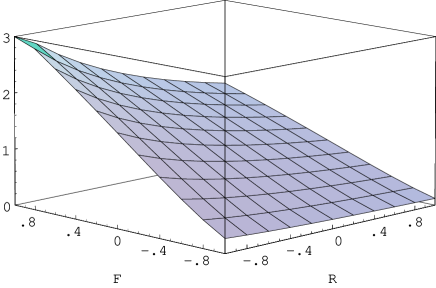
(a)

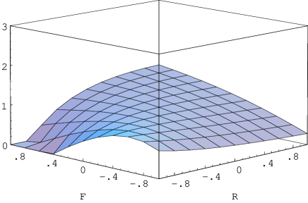
(b)

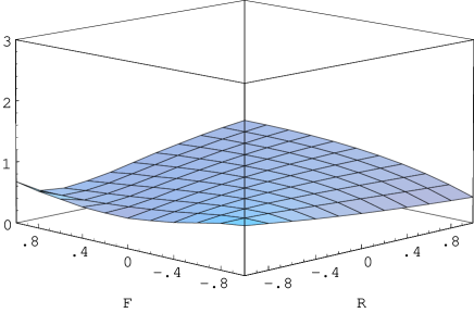
(c)

Figure 5: The cross section $\sigma(pp\to(b\bar{b})H+X)$ (in picobarns) at (a) LO, (b) NLO, (c) NNLO for the LHC. The axes labels are $F=\log_{10}(\mu_{F}/M_{H})$ and $R=\log_{10}(\mu_{R}/M_{H})$. Thus, the point $\mu_{R}=M_{H}$, $\mu_{F}=0.25\,M_{H}$ corresponds to $R=0$, $F=-0.6$. The Higgs boson mass is set to $M_{H}=120$ GeV.

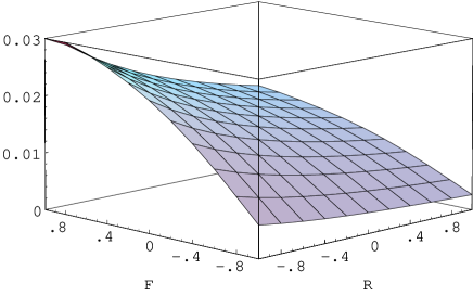
(a)

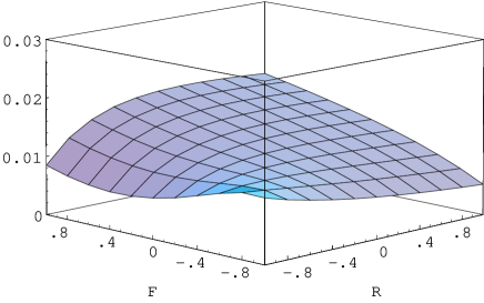
(b)

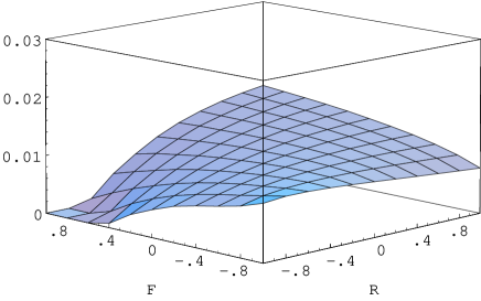
(c)

Figure 6: The cross section $\sigma(p\bar{p}\to(b\bar{b})H+X)$ (in picobarns) at (a) LO, (b) NLO, (c) NNLO for $\sqrt{s}=1.96$ GeV. The notation is the same as in Fig. 5. The Higgs boson mass is set to $M_{H}=120$ GeV.

$\beta_{i}^{m}$ and $\gamma_{i}$ have been defined in Eq. (12). Both $a_{s}(\mu)$ and $a_{s}(\mu_{0})$ are calculated from $\alpha_{s}(M_{Z})$ using the procedure described above. Working at LO (NLO, NNLO), we truncate the term in braces at order $a^{0}$ ($a^{1}$, $a^{2}$).

Convolution of the partonic cross section with the parton densities cancels the $\mu_{F}$ dependence up to higher orders and results in the physical hadronic cross section. The variation of the hadronic cross section with $\mu_{F}$ and $\mu_{R}$ is thus an indication of the size of higher order effects.

IV Results

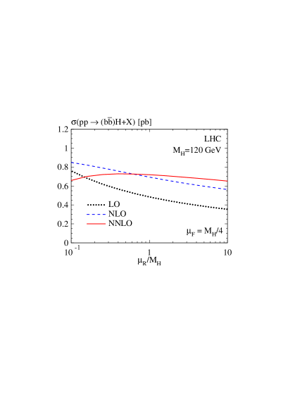
(a)

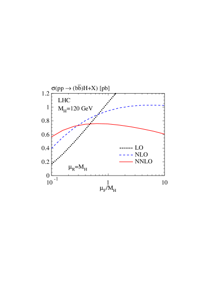
(b)

Figure 7: Cross section for $pp\to(b\bar{b})H+X$ at $\sqrt{s}=14$ TeV, $M_{H}=120$ GeV. (a) $\mu_{R}$ dependence for $\mu_{F}=0.25M_{H}$; (b) $\mu_{F}$ dependence for $\mu_{R}=M_{H}$.

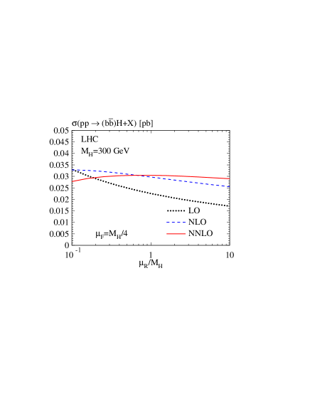
(a)

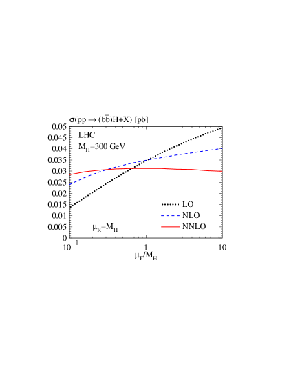
(b)

Figure 8: Cross section for $pp\to(b\bar{b})H+X$ at $\sqrt{s}=14$ TeV, $M_{H}=300$ GeV. (a) $\mu_{R}$ dependence for $\mu_{F}=0.25M_{H}$; (b) $\mu_{F}$ dependence for $\mu_{R}=M_{H}$.

The analytic expressions for the partonic cross section are quite voluminous and will be deferred to the appendix. In this section, we study the behavior of the NNLO result with respect to variations of the input parameters, in particular the Higgs boson mass and the collider type (LHC and Tevatron). Special emphasis is placed on the variation of the results with the renormalization and factorization scale, from which we estimate the theoretical uncertainty of the prediction for Higgs boson production in $b\bar{b}$ annihilation.

Because the cross sections for the neutral Higgs bosons in $b\bar{b}$ annihilation differ only in the magnitudes of the Yukawa couplings (within our approximations), we will restrict our discussion to the production of a Standard Model Higgs boson. In the limit that supersymmetric partners are heavy, their virtual contributions are insignificant and the predictions for supersymmetric Higgs bosons can be obtained from the Standard Model values by rescaling them with the proper coupling constants (cf. Eq. (10)).

All the numerical results have been obtained using Martin-Roberts-Stirling-Thorne (MRST) parton distributions. In particular, we use the MRST2001 sets Martin:2001es at LO $\left[\alpha_{s}(M_{Z})=0.130\right]$ and NLO $\left[\alpha_{s}(M_{Z})=0.119\right]$, and MRSTNNLO Martin:2002dr at NNLO $\left[\alpha_{s}(M_{Z})=0.1155\right]$.

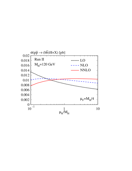
(a)

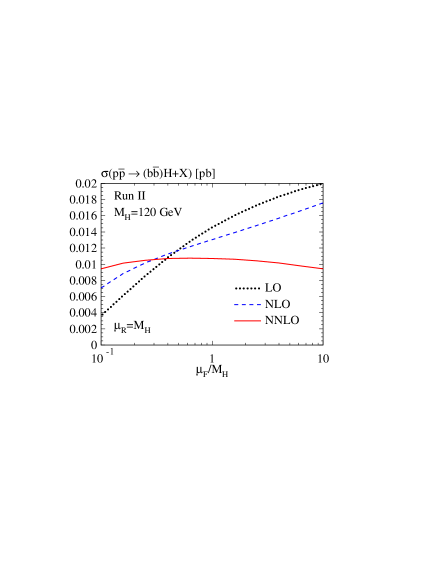
(b)

Figure 9: Cross section for $p\bar{p}\to(b\bar{b})H+X$ at $\sqrt{s}=1.96$ TeV, $M_{H}=120$ GeV. (a) $\mu_{R}$ dependence for $\mu_{F}=0.25M_{H}$; (b) $\mu_{F}$ dependence for $\mu_{R}=M_{H}$.

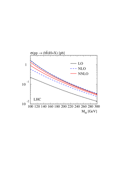
(a)

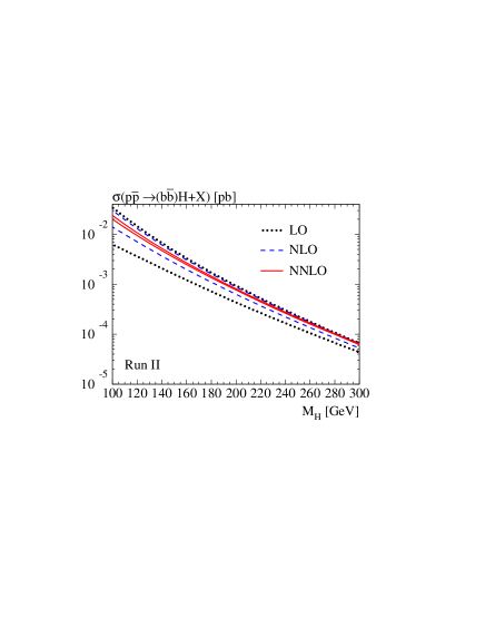
(b)

Figure 10: Cross section for Higgs boson production in bottom quark annihilation at (a) the LHC and (b) the Tevatron (Run II) at LO (dotted), NLO (dashed) and NNLO (solid). The upper (lower) line corresponds to a choice of the factorization scale of $\mu_{F}=0.7\,M_{H}$ ($\mu_{F}=0.1\,M_{H}$). The renormalization scale is set to $\mu_{R}=M_{H}$.

In order to obtain an overall picture of the renormalization and factorization scale dependence of the cross section, we plot $\sigma(pp\to(b\bar{b})H+X)$ for $\sqrt{s}=14$ TeV as a function of the two parameters $\mu_{F}$ and $\mu_{R}$ in Fig. 5. The corresponding plot for the Tevatron, i.e., $\sigma(p\bar{p}\to(b\bar{b})H+X)$ for $\sqrt{s}=1.96$ TeV, is shown in Fig. 6. The Higgs boson mass is fixed to $M_{H}=120$ GeV. Subpanels (a), (b), and (c) show the LO, NLO, and NNLO prediction, respectively. Note the extremely large variation of the scales, by a factor of 10 above and below $M_{H}$. Apart from the region of large $\mu_{F}$ and small $\mu_{R}$, one observes a clear reduction of the scale dependence with increasing order of perturbation theory, both for $\mu_{F}$ and $\mu_{R}$. Notably, we find minimal radiative corrections and a particularly weak dependence on the renormalization and factorization scales in the vicinity of $(\mu_{R},\mu_{F})=(M_{\phi},0.25\,M_{\phi})\equiv(\bar{\mu}_{R},\bar{\mu}_{F})$. This agrees with the observation of Ref. Maltoni:2003pn that the proper factorization scale for this process should be around $\mu_{F}=M_{\phi}/4$.

To illustrate this observation, we display separately the $\mu_{R}$- and $\mu_{F}$-variation of the cross section at the LHC in Fig. 7 for $M_{H}=120$ GeV, and in Fig. 8 for $M_{H}=300$ GeV. In subpanels (a), the factorization scale is fixed to $\mu_{F}=\bar{\mu}_{F}=0.25\,M_{H}$, and the renormalization scale is varied within $0.1\leq\mu_{R}/M_{H}\leq 10$. In subpanels (b), the renormalization scale is fixed to $\mu_{R}=\bar{\mu}_{R}=M_{H}$, and the factorization scale is varied within $0.1\leq\mu_{F}/M_{H}\leq 10$. The reduction in the scale dependence with increasing order of perturbation theory is clearly visible. As opposed to the lower order curves which have a monotonic dependence on $\mu_{R/F}$ within the displayed range, the NNLO curves develop a maximum, so that it is possible to define a “point of least sensitivity” for them. In all cases, this falls nicely into a region where the radiative corrections are small. Note also that the central values for the NNLO curves are perfectly consistent between panels (a) and (b). These observations confirm that $\bar{\mu}_{F}=0.25\,M_{H}$ and $\bar{\mu}_{R}=M_{H}$ are indeed the appropriate scale choices for this process.

The corresponding curves for Run II at the Tevatron are shown in Fig. 9 (we only show results at the Tevatron for $M_{H}=120$ GeV). As opposed to the LHC, the reduction of the renormalization scale dependence with increasing order of perturbation theory is less drastic. One even observes a slight increase in the $\mu_{R}$ dependence between NLO and NNLO. However, the absolute variation is very small. The factorization scale dependence is quite similar to that observed for the LHC. Again, the central values for the NNLO curves of subpanels (a) and (b) coincide nicely. Note that the cross section at the Tevatron is typically about two orders of magnitude smaller than at the LHC.

Fig. 10(a) shows the LO, NLO, and NNLO predictions for the cross section $\sigma(pp\to(b\bar{b})H+X)$ at the LHC as a function of the Higgs boson mass. The two curves at each order correspond to two different choices of the factorization scale, $\mu_{F}=0.1\,M_{H}$ and $\mu_{F}=0.7\,M_{H}$. From subpanels (b) of Figs. 7 and 8 one can see that this roughly defines the maximal $\mu_{F}$-variation at NNLO between $0.1\,M_{H}$ and $10\,M_{H}$. Since the renormalization scale dependence is very weak [cf. subpanels (a) of Figs. 7 and 8], we fix $\mu_{R}=\bar{\mu}_{R}=M_{H}$. Taking the width of these bands as an indication of the theoretical uncertainty, we observe an improvement of the accuracy of the prediction for $M_{H}=120$ GeV from $70\%$ at LO to $40\%$ at NLO to $15\%$ at NNLO. At larger Higgs boson masses, the scale uncertainty is smaller, amounting to $40\%$ at LO, $17\%$ at NLO, and $5\%$ at NNLO for $M_{H}=300$ GeV.

The cross section for the Tevatron at $\sqrt{s}=1.96$ TeV center-of-mass energy is shown in Fig. 10(b). Here the renormalization scale dependence within the range $0.1\leq\mu_{R}/M_{H}\leq 10$ at NNLO is larger than the factorization scale dependence (cf. Fig. 9). Nevertheless, we apply the same prescription as for the LHC and plot the LO, NLO, and NNLO cross section at $(\mu_{R},\mu_{F})=(1,0.1)\,M_{H}$ and $(\mu_{R},\mu_{F})=(1,0.7)\,M_{H}$. This is justified since $\mu_{R}$-variation on absolute scales is still very small, in particular if it is restricted to a more reasonable range of about a factor of five above and below $M_{H}$. We obtain a reduction of the scale uncertainty at the Tevatron for $M_{H}=120$ GeV from around $60\%$ at LO, to $30\%$ at NLO, to $10\%$ at NNLO.

V Conclusions

We have computed the total cross section for Higgs boson production in $b\bar{b}$ fusion at NNLO in QCD. We have argued that the NNLO plays an exceptional role in this process, as it incorporates all subleading logarithms at order $\alpha_{s}^{2}$. The results are very stable with respect to changes of the renormalization and factorization scales. We find that the radiative corrections are particularly small at factorization scales of around $\mu_{F}=M_{\phi}/4$, in agreement with the arguments of Refs. Plehn:2002vy ; Maltoni:2003pn .

We conclude that the inclusive cross section for Higgs boson production in bottom quark annihilation at hadron colliders is under good theoretical control.

Acknowledgments.

We would like to thank Scott Willenbrock, Fabio Maltoni, and Zack Sullivan for their encouragement and valuable comments. We are grateful to Tilman Plehn and Werner Vogelsang for enlightening discussions on bottom quark parton densities. R.V.H. would like to thank André Turcot for emphasizing the importance of this process, and Kostia Chetyrkin for useful comments. The work of W.B.K. was supported by the U. S. Department of Energy under Contract No. DE-AC02-98CH10886.

Appendix A Partonic results

It is convenient to write the partonic cross section in the following way:

$$\begin{split}\hat{\sigma}_{ij}(x)&=\sigma^{0}\,\Delta_{ij}(x)\,,\qquad i,j\in\{b,\bar{b},g,q,\bar{q}\}\,,\end{split}$$ (15)

where $\hat{\sigma}_{ij}$ is the cross section for the process $ij\to\phi+X$. $i$ and $j$ label the partons in the initial state, $\phi$ means either a scalar or pseudoscalar Higgs boson, and $X$ denotes any number of quarks or gluons in the final state. Here and in what follows, $q$ denotes any of the light quarks $u,d,s,c$. The normalization factor, $\sigma_{0}$, is

$$\sigma_{0}=\frac{\pi}{12}\frac{\lambda_{b}^{2}}{M_{\phi}^{2}}\,.$$ (16)

The correction terms are written as a perturbative expansion:

$$\Delta_{ij}(x)=\Delta_{ij}^{(0)}(x)+\frac{\alpha_{s}}{\pi}\,\Delta_{ij}^{(1)}(x)+\left(\frac{\alpha_{s}}{\pi}\right)^{2}\,\Delta_{ij}^{(2)}(x)+{\cal O}(\alpha_{s}^{3})\,.$$ (17)

Explicit dependence on the number of active flavors $n_{f}$ appears only at NNLO. Because the terms are large and cumbersome, it is convenient to write

$$\Delta_{ij}^{(2)}(x)=\Delta_{ij}^{(2)\,A}(x)+n_{f}\,\Delta_{ij}^{(2)\,F}(x)\,.$$ (18)

All results will be presented for the scale choices $\mu_{F}=\mu_{R}=M_{\phi}$. The corresponding expressions for general values of $\mu_{F}$ and $\mu_{R}$ can be reconstructed from renormalization scale invariance of the partonic, and factorization invariance of the hadronic cross section.

A.1 The $b\bar{b}$ subprocess

In the VFS approach, the tree-level $b\bar{b}$ annihilation term is the LO contribution. Thus, this is the only term for which $\Delta_{ij}^{(0)}(x)$ does not vanish. The LO contribution to $b\bar{b}\to\phi+X$ is

$$\Delta_{b\bar{b}}^{(0)}(x)=\delta(1-x).$$ (19)

The NLO contribution is

$$\begin{split}\Delta_{b\bar{b}}^{(1)}(x)=&\ -\frac{4-8\,\zeta_{2}}{3}\,\delta(1-x)+\frac{16}{3}\,{\cal D}_{1}(1-x)-\frac{16+8\,x+8\,x^{2}}{3}\,\ln\left(1-x\right)+\frac{4\,x-4\,x^{2}}{3}-\frac{8}{3}\,\frac{\ln\left(x\right)}{1-x}+\frac{8+4\,x+4\,x^{2}}{3}\,\ln\left(x\right)\,,\end{split}$$ (20)

where $\displaystyle{\cal D}_{n}(1-x)\equiv\left[\frac{\ln^{n}(1-x)}{1-x}\right]_{+}$, and $\zeta_{2}\equiv\pi^{2}/6\approx 1.64493$, $\zeta_{3}\approx 1.20206$.

At NNLO, the contributions are ($\zeta_{4}\equiv\pi^{4}/90\approx 1.08232$)

$$\begin{split}\Delta_{b\bar{b}}^{(2)\,A}=&\ \frac{115+116\,\zeta_{2}-156\,\zeta_{3}-19\,\zeta_{4}}{18}\,\delta\left(1-x\right)-\frac{404-396\,\zeta_{2}-1146\,\zeta_{3}}{27}\,{\cal D}_{0}\left(1-x\right)\\ &+\frac{204-200\,\zeta_{2}}{9}\,{\cal D}_{1}\left(1-x\right)-\frac{44}{3}\,{\cal D}_{2}\left(1-x\right)+\frac{128}{9}\,{\cal D}_{3}\left(1-x\right)\\ &-\frac{128+64\,x+64\,x^{2}}{9}\,\ln^{3}\left(1-x\right)+\frac{140+40\,x+92\,x^{2}-8\,x^{3}}{9}\,\ln^{2}\left(1-x\right)\\ &-\frac{248}{9}\,\frac{\ln^{2}\left(1-x\right)\,\ln\left(x\right)}{1-x}+\frac{248+168\,x+168\,x^{2}}{9}\,\ln^{2}\left(1-x\right)\,\ln\left(x\right)\\ &-\frac{604+138\,x+423\,x^{2}+44\,x^{3}}{27}\,\ln\left(1-x\right)+\frac{200+100\,x+100\,x^{2}}{9}\,\zeta_{2}\,\ln\left(1-x\right)\\ &+24\,\frac{\ln\left(1-x\right)\,\ln\left(x\right)}{1-x}-\frac{216+110\,x+160\,x^{2}-24\,x^{3}}{9}\,\ln\left(1-x\right)\,\ln\left(x\right)\\ &+\frac{148}{9}\,\frac{\ln\left(1-x\right)\,\ln^{2}\left(x\right)}{1-x}-\frac{148+110\,x+110\,x^{2}}{9}\,\ln\left(1-x\right)\,\ln^{2}\left(x\right)\\ &+\frac{20}{9}\,\frac{\ln\left(1-x\right)\,{\mathop{\rm Li}_{2}\nolimits}\left(1-x\right)}{1-x}-\frac{20-78\,x-78\,x^{2}}{9}\,\ln\left(1-x\right)\,{\mathop{\rm Li}_{2}\nolimits}\left(1-x\right)\\ &+\frac{4640+1017\,x+2958\,x^{2}+721\,x^{3}}{324}-\frac{140-15\,x+147\,x^{2}-8\,x^{3}}{9}\,\zeta_{2}\\ &-\frac{382+191\,x+191\,x^{2}}{9}\,\zeta_{3}-\frac{146}{9}\,\frac{\ln\left(x\right)}{1-x}+\frac{164}{9}\,\frac{\zeta_{2}\,\ln\left(x\right)}{1-x}-\frac{23}{3}\,\frac{\ln^{2}\left(x\right)}{1-x}-\frac{44}{27}\,\frac{\ln^{3}\left(x\right)}{1-x}\\ &+\frac{876+249\,x+444\,x^{2}+38\,x^{3}}{54}\,\ln\left(x\right)-\frac{164+126\,x+126\,x^{2}}{9}\,\zeta_{2}\,\ln\left(x\right)\\ &+\frac{138+73\,x+115\,x^{2}-12\,x^{3}}{18}\,\ln^{2}\left(x\right)+\frac{44+21\,x+21\,x^{2}+4\,x^{3}}{27}\,\ln^{3}\left(x\right)\\ &+\frac{{\mathop{\rm Li}_{2}\nolimits}\left(1-x\right)}{1-x}+\frac{58}{9}\,\frac{{\mathop{\rm Li}_{2}\nolimits}\left(1-x\right)\,\ln\left(x\right)}{1-x}-\frac{142}{9}\,\frac{{\mathop{\rm Li}_{3}\nolimits}\left(1-x\right)}{1-x}-\frac{64}{9\,\left(1-x\right)}\,{\mathop{\rm Li}_{3}\nolimits}\left(-\frac{1-x}{x}\right)\\ &+\frac{7-51\,x-10\,x^{2}+10\,x^{3}}{9}\,{\mathop{\rm Li}_{2}\nolimits}\left(1-x\right)-\frac{58+88\,x+88\,x^{2}+2\,x^{3}}{9}\,{\mathop{\rm Li}_{2}\nolimits}\left(1-x\right)\,\ln\left(x\right)\\ &-\frac{x-2\,x^{2}-2\,x^{3}}{9}\,{\mathop{\rm Li}_{2}\nolimits}\left(1-x^{2}\right)+\frac{x^{3}}{3}\,{\mathop{\rm Li}_{2}\nolimits}\left(1-x^{2}\right)\,\ln\left(x\right)\\ &+\frac{142+37\,x+37\,x^{2}+6\,x^{3}}{9}\,{\mathop{\rm Li}_{3}\nolimits}\left(1-x\right)+\frac{64+94\,x+94\,x^{2}-6\,x^{3}}{9}\,{\mathop{\rm Li}_{3}\nolimits}\left(-\frac{1-x}{x}\right)\\ &-\frac{7\,x^{3}}{18}\,{\mathop{\rm Li}_{3}\nolimits}\left(1-x^{2}\right)-\frac{x^{3}}{18}\,{\mathop{\rm Li}_{3}\nolimits}\left(-\frac{1-x^{2}}{x^{2}}\right)-\frac{2\,x^{3}}{3}\,\left[{\mathop{\rm Li}_{3}\nolimits}\left(\frac{1-x}{1+x}\right)-{\mathop{\rm Li}_{3}\nolimits}\left(-\frac{1-x}{1+x}\right)\right]\,,\end{split}$$ (21)

$$\begin{split}\Delta_{b\bar{b}}^{(2)\,F}=&\ \frac{2-10\,\zeta_{2}+18\,\zeta_{3}}{27}\,\delta\left(1-x\right)+\frac{56-72\,\zeta_{2}}{81}\,{\cal D}_{0}\left(1-x\right)-\frac{40}{27}\,{\cal D}_{1}\left(1-x\right)+\frac{8}{9}\,{\cal D}_{2}\left(1-x\right)\\ &-\frac{8+4\,x+4\,x^{2}}{9}\,\ln^{2}\left(1-x\right)+\frac{40+8\,x+32\,x^{2}}{27}\,\ln\left(1-x\right)-\frac{16}{9}\,\frac{\ln\left(1-x\right)\,\ln\left(x\right)}{1-x}\\ &+\frac{16+8\,x+8\,x^{2}}{9}\,\ln\left(1-x\right)\,\ln\left(x\right)+\frac{10}{9}\,\frac{\ln\left(x\right)}{1-x}+\frac{2}{3}\,\frac{\ln^{2}\left(x\right)}{1-x}-\frac{2}{9}\,\frac{{\mathop{\rm Li}_{2}\nolimits}\left(1-x\right)}{1-x}-\frac{56+x+55\,x^{2}}{81}\\ &+\frac{8+4\,x+4\,x^{2}}{9}\,\zeta_{2}-\frac{10+3\,x+7\,x^{2}}{9}\,\ln\left(x\right)-\frac{12+7\,x+7\,x^{2}}{18}\,\ln^{2}\left(x\right)+\frac{2}{9}\,{\mathop{\rm Li}_{2}\nolimits}\left(1-x\right)\,.\end{split}$$ (22)

Note that the ${\cal D}_{n}$ terms in this result could also be derived by other methods Kramer:1998iq ; Vogt:2000ci ; Harlander:2001is ; Catani:2001ic ; Kidonakis:2003tx ; Magnea:1991qg ; Contopanagos:1997nh .

A.2 The $bg$ subprocess

The $bg\to\phi+X$ subprocess first enters at NLO, where the contribution is

$$\begin{split}&\Delta_{bg}^{(1)}=\Delta_{\bar{b}g}^{(1)}=\frac{x-2\,x^{2}+2\,x^{3}}{2}\,\ln\left(1-x\right)-\frac{3\,x-10\,x^{2}+7\,x^{3}}{8}-\frac{x-2\,x^{2}+2\,x^{3}}{4}\,\ln\left(x\right)\,.\end{split}$$ (23)

At NNLO, the contribution is

$$\begin{split}&\Delta_{bg}^{(2)\,A}=\Delta_{\bar{b}g}^{(2)\,A}=\\ &\phantom{+}\frac{257\,x-514\,x^{2}+514\,x^{3}}{144}\,\ln^{3}\left(1-x\right)\\ &+\frac{16-59\,x+272\,x^{2}-237\,x^{3}}{16}\,\ln^{2}\left(1-x\right)-\frac{11\,x-94\,x^{2}+62\,x^{3}}{8}\,\ln^{2}\left(1-x\right)\,\ln\left(x\right)\\ &+\frac{16+28\,x-731\,x^{2}+726\,x^{3}}{48}\,\ln\left(1-x\right)-\frac{35\,x-70\,x^{2}+70\,x^{3}}{12}\,\zeta_{2}\,\ln\left(1-x\right)\\ &+\frac{65\,x-508\,x^{2}+774\,x^{3}}{24}\,\ln\left(1-x\right)\,\ln\left(x\right)-\frac{3\,x+174\,x^{2}-98\,x^{3}}{24}\,\ln\left(1-x\right)\,\ln^{2}\left(x\right)\\ &+\frac{77\,x+134\,x^{2}-86\,x^{3}}{24}\,\ln\left(1-x\right)\,{\mathop{\rm Li}_{2}\nolimits}\left(1-x\right)+\frac{3\,x+6\,x^{2}+6\,x^{3}}{4}\,\ln\left(1-x\right)\,{\mathop{\rm Li}_{2}\nolimits}\left(1-x^{2}\right)\\ &-\frac{208-411\,x-1350\,x^{2}+1781\,x^{3}}{288}-\frac{16-31\,x+176\,x^{2}-169\,x^{3}}{16}\,\zeta_{2}+\frac{161\,x-322\,x^{2}+322\,x^{3}}{48}\,\zeta_{3}\\ &+\frac{32\,x+536\,x^{2}-993\,x^{3}}{48}\,\ln\left(x\right)+\frac{7\,x-230\,x^{2}+134\,x^{3}}{24}\,\zeta_{2}\,\ln\left(x\right)\\ &-\frac{47\,x-604\,x^{2}+1028\,x^{3}}{96}\,\ln^{2}\left(x\right)-\frac{35\,x+146\,x^{2}+12\,x^{3}}{144}\,\ln^{3}\left(x\right)\\ &+\frac{48-43\,x+152\,x^{2}+236\,x^{3}}{24}\,{\mathop{\rm Li}_{2}\nolimits}\left(1-x\right)-\frac{10\,x+34\,x^{2}-17\,x^{3}}{6}\,{\mathop{\rm Li}_{2}\nolimits}\left(1-x\right)\,\ln\left(x\right)\\ &-\frac{19\,x+40\,x^{2}+21\,x^{3}}{48}\,{\mathop{\rm Li}_{2}\nolimits}\left(1-x^{2}\right)-\frac{9\,x+18\,x^{2}+10\,x^{3}}{12}\,{\mathop{\rm Li}_{2}\nolimits}\left(1-x^{2}\right)\,\ln\left(x\right)\\ &-\frac{14\,x+8\,x^{2}+9\,x^{3}}{3}\,{\mathop{\rm Li}_{3}\nolimits}\left(1-x\right)+\frac{13\,x+118\,x^{2}-18\,x^{3}}{12}\,{\mathop{\rm Li}_{3}\nolimits}\left(-\frac{1-x}{x}\right)\\ &+\frac{9\,x+18\,x^{2}-14\,x^{3}}{48}\,{\mathop{\rm Li}_{3}\nolimits}\left(1-x^{2}\right)+\frac{9\,x+18\,x^{2}-14\,x^{3}}{48}\,{\mathop{\rm Li}_{3}\nolimits}\left(-\frac{1-x^{2}}{x^{2}}\right)\\ &+\frac{3\,x+6\,x^{2}+6\,x^{3}}{2}\,\left[{\mathop{\rm Li}_{3}\nolimits}\left(\frac{1-x}{1+x}\right)-{\mathop{\rm Li}_{3}\nolimits}\left(-\frac{1-x}{1+x}\right)\right]\,,\\[10.00002pt] \Delta_{bg}^{(2)\,F}=&\ \Delta_{\bar{b}g}^{(2)\,F}=0\,.\end{split}$$ (24)

A.3 The $bq$ subprocess

All remaining components contribute only at NNLO and beyond. The contribution to $bq\to\phi+X$, where $q$ is a light ($u$,$d$,$s$ or $c$) quark, is:

$$\begin{split}\Delta_{bq}^{(2)\,A}=&\ \Delta_{\bar{b}q}^{(2)\,A}=\Delta_{b\bar{q}}^{(2)\,A}=\Delta_{\bar{b}\bar{q}}^{(2)\,A}=\frac{4+3\,x-3\,x^{2}-4\,x^{3}}{9}\,\ln^{2}\left(1-x\right)\\ &+\frac{2\,x+2\,x^{2}}{3}\,\ln^{2}\left(1-x\right)\,\ln\left(x\right)+\frac{4-57\,x+75\,x^{2}-22\,x^{3}}{27}\,\ln\left(1-x\right)\\ &-\frac{x-4\,x^{2}-4\,x^{3}}{3}\,\ln\left(1-x\right)\,\ln\left(x\right)-\frac{2\,x+2\,x^{2}}{3}\,\ln\left(1-x\right)\,\ln^{2}\left(x\right)\\ &+\frac{4\,x+4\,x^{2}}{3}\,\ln\left(1-x\right)\,{\mathop{\rm Li}_{2}\nolimits}\left(1-x\right)-\frac{208-915\,x+1410\,x^{2}-703\,x^{3}}{648}\\ &-\frac{4+3\,x-3\,x^{2}-4\,x^{3}}{9}\,\zeta_{2}+\frac{93\,x-264\,x^{2}+20\,x^{3}}{108}\,\ln\left(x\right)-\frac{2\,x+2\,x^{2}}{3}\,\zeta_{2}\,\ln\left(x\right)\\ &-\frac{3\,x+15\,x^{2}+40\,x^{3}}{72}\,\ln^{2}\left(x\right)+\frac{x+x^{2}}{36}\,\ln^{3}\left(x\right)+\frac{16-3\,x+21\,x^{2}+8\,x^{3}}{18}\,{\mathop{\rm Li}_{2}\nolimits}\left(1-x\right)\\ &-\left(x+x^{2}\right)\,{\mathop{\rm Li}_{2}\nolimits}\left(1-x\right)\,\ln\left(x\right)-\frac{2\,x+2\,x^{2}}{3}\,{\mathop{\rm Li}_{3}\nolimits}\left(1-x\right)+\frac{2\,x+2\,x^{2}}{3}\,{\mathop{\rm Li}_{3}\nolimits}\left(-\frac{1-x}{x}\right)\,,\\[10.00002pt] \Delta_{bq}^{(2)\,F}=&\ \Delta_{\bar{b}q}^{(2)\,F}=\Delta_{b\bar{q}}^{(2)\,F}=\Delta_{\bar{b}\bar{q}}^{(2)\,F}=0\,.\end{split}$$ (25)

A.4 The $gg$ subprocess

The contribution to $gg\to\phi+X$ is:

$$\begin{split}\Delta_{gg}^{(2)\,A}=&\ -\left(x+2\,x^{2}-3\,x^{3}\right)\,\ln^{2}\left(1-x\right)-\frac{x+4\,x^{2}+4\,x^{3}}{2}\,\ln^{2}\left(1-x\right)\,\ln\left(x\right)\\ &+\frac{23\,x+52\,x^{2}-75\,x^{3}}{8}\,\ln\left(1-x\right)+\frac{5\,x+16\,x^{2}-4\,x^{3}}{4}\,\ln\left(1-x\right)\,\ln\left(x\right)\\ &+\frac{x+4\,x^{2}+4\,x^{3}}{4}\,\ln\left(1-x\right)\,\ln^{2}\left(x\right)-\left(x+4\,x^{2}+4\,x^{3}\right)\,\ln\left(1-x\right)\,{\mathop{\rm Li}_{2}\nolimits}\left(1-x\right)\\ &-\frac{163\,x+1528\,x^{2}-1691\,x^{3}}{128}+\left(x+2\,x^{2}-3\,x^{3}\right)\,\zeta_{2}\\ &-\frac{54\,x+312\,x^{2}-223\,x^{3}}{64}\,\ln\left(x\right)+\frac{x+4\,x^{2}+4\,x^{3}}{2}\,\zeta_{2}\,\ln\left(x\right)\\ &-\frac{16\,x+111\,x^{2}-43\,x^{3}}{64}\,\ln^{2}\left(x\right)+\frac{7\,x+25\,x^{2}+34\,x^{3}}{48}\,\ln^{3}\left(x\right)\\ &-\frac{4\,x-15\,x^{2}-62\,x^{3}}{16}\,{\mathop{\rm Li}_{2}\nolimits}\left(1-x\right)+\frac{11\,x+44\,x^{2}+30\,x^{3}}{16}\,{\mathop{\rm Li}_{2}\nolimits}\left(1-x\right)\,\ln\left(x\right)\\ &+\frac{x^{2}-6\,x^{3}}{32}\,{\mathop{\rm Li}_{2}\nolimits}\left(1-x^{2}\right)+\frac{3\,x+6\,x^{2}+38\,x^{3}}{64}\,{\mathop{\rm Li}_{2}\nolimits}\left(1-x^{2}\right)\,\ln\left(x\right)\\ &+\frac{x+3\,x^{2}+18\,x^{3}}{8}\,{\mathop{\rm Li}_{3}\nolimits}\left(1-x\right)-\frac{15\,x+60\,x^{2}+30\,x^{3}}{16}\,{\mathop{\rm Li}_{3}\nolimits}\left(-\frac{1-x}{x}\right)\\ &-\frac{5\,x+10\,x^{2}+74\,x^{3}}{128}\,{\mathop{\rm Li}_{3}\nolimits}\left(1-x^{2}\right)-\frac{3\,x+6\,x^{2}+70\,x^{3}}{128}\,{\mathop{\rm Li}_{3}\nolimits}\left(-\frac{1-x^{2}}{x^{2}}\right)\\ &-\frac{x+2\,x^{2}+2\,x^{3}}{32}\,\left[{\mathop{\rm Li}_{3}\nolimits}\left(\frac{1-x}{1+x}\right)-{\mathop{\rm Li}_{3}\nolimits}\left(-\frac{1-x}{1+x}\right)\right]\,,\\[10.00002pt] \Delta_{gg}^{(2)\,F}=&\ 0\,.\end{split}$$ (26)

A.5 The $bb$ subprocess

The contribution to $bb\to\phi+X$ is:

$$\begin{split}\Delta_{bb}^{(2)\,A}=&\ \Delta_{\bar{b}\bar{b}}^{(2)\,A}=\frac{8+6\,x-6\,x^{2}-8\,x^{3}}{9}\,\ln^{2}\left(1-x\right)+\frac{4\,x+4\,x^{2}}{3}\,\ln^{2}\left(1-x\right)\,\ln\left(x\right)\\ &+\frac{8-138\,x+174\,x^{2}-44\,x^{3}}{27}\,\ln\left(1-x\right)-\frac{10\,x-20\,x^{2}-24\,x^{3}}{9}\,\ln\left(1-x\right)\,\ln\left(x\right)\\ &+\frac{4}{9}\,\frac{\ln\left(1-x\right)\,\ln^{2}\left(x\right)}{1+x}-\frac{16}{9}\,\frac{\ln\left(1-x\right)\,{\mathop{\rm Li}_{2}\nolimits}\left(1-x\right)}{1+x}+\frac{8}{9}\,\frac{\ln\left(1-x\right)\,{\mathop{\rm Li}_{2}\nolimits}\left(1-x^{2}\right)}{1+x}\\ &-\frac{4+10\,x+14\,x^{2}}{9}\,\ln\left(1-x\right)\,\ln^{2}\left(x\right)+\frac{16+16\,x+32\,x^{2}}{9}\,\ln\left(1-x\right)\,{\mathop{\rm Li}_{2}\nolimits}\left(1-x\right)\\ &-\frac{8-4\,x+4\,x^{2}}{9}\,\ln\left(1-x\right)\,{\mathop{\rm Li}_{2}\nolimits}\left(1-x^{2}\right)-\frac{52-357\,x+510\,x^{2}-205\,x^{3}}{81}\\ &-\frac{8+6\,x-6\,x^{2}-8\,x^{3}}{9}\,\zeta_{2}+\frac{117\,x-279\,x^{2}+20\,x^{3}}{54}\,\ln\left(x\right)-\frac{4\,x+4\,x^{2}}{3}\,\zeta_{2}\,\ln(x)\\ &-\frac{x+11\,x^{2}+34\,x^{3}}{36}\,\ln^{2}(x)+\frac{28-12\,x+17\,x^{2}}{54}\,\ln^{3}\left(x\right)-\frac{14}{27}\,\frac{\ln^{3}\left(x\right)}{1+x}\\ &+\frac{4}{3}\,\frac{{\mathop{\rm Li}_{2}\nolimits}\left(1-x\right)\,\ln\left(x\right)}{1+x}-\frac{8}{9}\,\frac{{\mathop{\rm Li}_{2}\nolimits}\left(1-x^{2}\right)\,\ln\left(x\right)}{1+x}-\frac{4}{3}\,\frac{{\mathop{\rm Li}_{3}\nolimits}\left(1-x\right)}{1+x}+\frac{4}{3\,\left(1+x\right)}\,{\mathop{\rm Li}_{3}\nolimits}\left(-\frac{1-x}{x}\right)\\ &+\frac{1}{3}\,\frac{{\mathop{\rm Li}_{3}\nolimits}\left(1-x^{2}\right)}{1+x}+\frac{1}{9\,\left(1+x\right)}\,{\mathop{\rm Li}_{3}\nolimits}\left(-\frac{1-x^{2}}{x^{2}}\right)+\frac{20}{9\,\left(1+x\right)}\,\left[{\mathop{\rm Li}_{3}\nolimits}\left(\frac{1-x}{1+x}\right)-{\mathop{\rm Li}_{3}\nolimits}\left(-\frac{1-x}{1+x}\right)\right]\\ &+\frac{16-12\,x+16\,x^{2}+11\,x^{3}}{9}\,{\mathop{\rm Li}_{2}\nolimits}\left(1-x\right)-\frac{12+8\,x+29\,x^{2}}{9}\,{\mathop{\rm Li}_{2}\nolimits}\left(1-x\right)\,\ln\left(x\right)\\ &+\frac{x}{9}\,{\mathop{\rm Li}_{2}\nolimits}\left(1-x^{2}\right)+\frac{16-11\,x+11\,x^{2}}{18}\,{\mathop{\rm Li}_{2}\nolimits}\left(1-x^{2}\right)\,\ln\left(x\right)+\frac{12-27\,x+5\,x^{2}}{9}\,{\mathop{\rm Li}_{3}\nolimits}\left(1-x\right)\\ &-\frac{12-16\,x-9\,x^{2}-2\,x^{3}}{9}\,{\mathop{\rm Li}_{3}\nolimits}\left(-\frac{1-x}{x}\right)-\frac{12-13\,x+13\,x^{2}}{36}\,{\mathop{\rm Li}_{3}\nolimits}\left(1-x^{2}\right)\\ &-\frac{4-3\,x+3\,x^{2}}{36}\,{\mathop{\rm Li}_{3}\nolimits}\left(-\frac{1-x^{2}}{x^{2}}\right)-\frac{20-13\,x+13\,x^{2}}{9}\,\left[{\mathop{\rm Li}_{3}\nolimits}\left(\frac{1-x}{1+x}\right)-{\mathop{\rm Li}_{3}\nolimits}\left(-\frac{1-x}{1+x}\right)\right]\,,\\[10.00002pt] \Delta_{bb}^{(2)\,F}=&\ \Delta_{\bar{b}\bar{b}}^{(2)\,F}=0\,.\end{split}$$ (27)

A.6 The $q\bar{q}$ subprocess

The contribution to $q\bar{q}\to\phi+X$ is ($q\in\{u,d,s,c\}$):

$$\begin{split}\Delta_{q\bar{q}}^{(2)\,A}=&\ -\frac{2\,x-8\,x^{2}+6\,x^{3}}{9}-\frac{x-2\,x^{2}-3\,x^{3}}{9}\,\ln\left(x\right)+\frac{x^{3}}{9}\,\ln^{2}\left(x\right)\hskip 72.26999pt\\ &\ -\frac{4\,x^{3}}{9}\,{\mathop{\rm Li}_{2}\nolimits}\left(1-x\right)+\frac{2\,x^{3}}{9}\,{\mathop{\rm Li}_{2}\nolimits}\left(1-x^{2}\right)\,,\\[10.00002pt] \Delta_{q\bar{q}}^{(2)\,F}=&\ 0\,.\end{split}$$ (28)

References

- (1) The luminosity monitor of Tevatron Run II can be found at http://www.fnal.gov/pub/now/tevlum.html.
- (2) M. Carena and H. E. Haber, Higgs boson theory and phenomenology, http://arXiv.org/abs/hep-ph/0208209.
- (3) R. V. Harlander and W. B. Kilgore, Next-to-next-to-leading order Higgs production at hadron colliders, Phys. Rev. Lett. 88 (2002) 201801, [ http://arXiv.org/abs/hep-ph/0201206].
- (4) C. Anastasiou and K. Melnikov, Higgs boson production at hadron colliders in NNLO QCD, Nucl. Phys. B646 (2002) 220–256, [ http://arXiv.org/abs/hep-ph/0207004].
- (5) V. Ravindran, J. Smith, and W. L. van Neerven, NNLO corrections to the total cross section for Higgs boson production in hadron hadron collisions, http://arXiv.org/abs/hep-ph/0302135.
- (6) T. Han, G. Valencia, and S. Willenbrock, Structure function approach to vector-boson scattering in collisions, Phys. Rev. Lett. 69 (1992) 3274–3277, [ http://arXiv.org/abs/hep-ph/9206246].
- (7) T. Han and S. Willenbrock, QCD correction to the and total cross-sections, Phys. Lett. B273 (1991) 167–172.
- (8) L. Reina and S. Dawson, Next-to-leading order results for production at the Tevatron, Phys. Rev. Lett. 87 (2001) 201804, [ http://arXiv.org/abs/hep-ph/0107101].
- (9) W. Beenakker et. al., Higgs radiation off top quarks at the Tevatron and the LHC, Phys. Rev. Lett. 87 (2001) 201805, [ http://arXiv.org/abs/hep-ph/0107081].
- (10) S. Dawson, L. H. Orr, L. Reina, and D. Wackeroth, Associated top quark-Higgs boson production at the LHC, Phys. Rev. D67 (2003) 071503, [ http://arXiv.org/abs/hep-ph/0211438].
- (11) W. Beenakker et. al., NLO QCD corrections to production in hadron collisions, Nucl. Phys. B653 (2003) 151–203, [ http://arXiv.org/abs/hep-ph/0211352].
- (12) S. Dawson, A. Djouadi, and M. Spira, QCD corrections to SUSY Higgs production: The role of squark loops, Phys. Rev. Lett. 77 (1996) 16–19, [ http://arXiv.org/abs/hep-ph/9603423].
- (13) S. P. Martin, A supersymmetry primer, http://arXiv.org/abs/hep-ph/9709356.
- (14) M. Spira, A. Djouadi, D. Graudenz, and P. M. Zerwas, Higgs boson production at the LHC, Nucl. Phys. B453 (1995) 17–82, [ http://arXiv.org/abs/hep-ph/9504378].
- (15) D. A. Dicus and S. Willenbrock, Higgs boson production from heavy quark fusion, Phys. Rev. D39 (1989) 751.
- (16) D. Dicus, T. Stelzer, Z. Sullivan, and S. Willenbrock, Higgs boson production in association with bottom quarks at next-to-leading order, Phys. Rev. D59 (1999) 094016, [ http://arXiv.org/abs/hep-ph/9811492].
- (17) F. Maltoni, Z. Sullivan, and S. Willenbrock, Higgs-boson production via bottom-quark fusion, Phys. Rev. D67 (2003) 093005, [ http://arXiv.org/abs/hep-ph/0301033].
- (18) R. M. Barnett, H. E. Haber, and D. E. Soper, Ultraheavy particle production from heavy partons at hadron colliders, Nucl. Phys. B306 (1988) 697.
- (19) F. I. Olness and W.-K. Tung, When is a heavy quark not a parton? charged Higgs production and heavy quark mass effects in the QCD based parton model, Nucl. Phys. B308 (1988) 813.
- (20) M. A. G. Aivazis, J. C. Collins, F. I. Olness, and W.-K. Tung, Leptoproduction of heavy quarks. II. a unified QCD formulation of charged and neutral current processes from fixed-target to collider energies, Phys. Rev. D50 (1994) 3102–3118, [ http://arXiv.org/abs/hep-ph/9312319].
- (21) R. S. Thorne and R. G. Roberts, An ordered analysis of heavy flavour production in deep inelastic scattering, Phys. Rev. D57 (1998) 6871–6898, [ http://arXiv.org/abs/hep-ph/9709442].
- (22) M. Krämer, F. I. Olness, and D. E. Soper, Treatment of heavy quarks in deeply inelastic scattering, Phys. Rev. D62 (2000) 096007, [ http://arXiv.org/abs/hep-ph/0003035].
- (23) M. Buza, Y. Matiounine, J. Smith, R. Migneron, and W. L. van Neerven, Heavy quark coefficient functions at asymptotic values , Nucl. Phys. B472 (1996) 611–658, [ http://arXiv.org/abs/hep-ph/9601302].
- (24) M. Buza, Y. Matiounine, J. Smith, and W. L. van Neerven, Charm electroproduction viewed in the variable-flavour number scheme versus fixed-order perturbation theory, Eur. Phys. J. C1 (1998) 301–320, [ http://arXiv.org/abs/hep-ph/9612398].
- (25) A. Chuvakin, J. Smith, and W. L. van Neerven, Comparison between variable flavor number schemes for charm quark electroproduction, Phys. Rev. D61 (2000) 096004, [ http://arXiv.org/abs/hep-ph/9910250].
- (26) A. Chuvakin and J. Smith, Modified minimal subtraction scheme parton densities with nnlo heavy flavor matching conditions, Phys. Rev. D61 (2000) 114018, [ http://arXiv.org/abs/hep-ph/9911504].
- (27) A. Chuvakin, J. Smith, and W. L. van Neerven, Bottom quark electroproduction in variable flavor number schemes, Phys. Rev. D62 (2000) 036004, [ http://arXiv.org/abs/hep-ph/0002011].
- (28) A. Chuvakin, J. Smith, and B. W. Harris, Variable flavor number schemes versus fixed order perturbation theory for charm quark electroproduction, Eur. Phys. J. C18 (2001) 547–553, [ http://arXiv.org/abs/hep-ph/0010350].
- (29) E. Eichten, I. Hinchliffe, K. D. Lane, and C. Quigg, Super collider physics, Rev. Mod. Phys. 56 (1984) 579–707.
- (30) J. F. Gunion, H. E. Haber, F. E. Paige, W.-K. Tung, and S. S. D. Willenbrock, Neutral and charged Higgs detection: Heavy quark fusion, top quark mass dependence and rare decays, Nucl. Phys. B294 (1987) 621.
- (31) R. Raitio and W. W. Wada, Higgs boson production at large transverse momentum in QCD, Phys. Rev. D19 (1979) 941.
- (32) J. N. Ng and P. Zakarauskas, QCD-parton calculation of conjoined production of Higgs bosons and heavy flavors in collisions, Phys. Rev. D29 (1984) 876.
- (33) Z. Kunszt, Associated production of heavy Higgs boson with top quarks, Nucl. Phys. B247 (1984) 339.
- (34) J. Campbell, R. K. Ellis, F. Maltoni, and S. Willenbrock, Higgs boson production in association with a single bottom quark, Phys. Rev. D67 (2003) 095002, [ http://arXiv.org/abs/hep-ph/0204093].
- (35) C. Balazs, H.-J. He, and C. P. Yuan, QCD corrections to scalar production via heavy quark fusion at hadron colliders, Phys. Rev. D60 (1999) 114001, [ http://arXiv.org/abs/hep-ph/9812263].
- (36) D. Rainwater, M. Spira, and D. Zeppenfeld, Higgs boson production at hadron colliders: Signal and background processes, http://arXiv.org/abs/hep-ph/0203187.
- (37) M. Spira, Higgs and SUSY particle production at hadron colliders, http://arXiv.org/abs/hep-ph/0211145.
- (38) T. Plehn, Charged Higgs boson production in bottom gluon fusion, Phys. Rev. D67 (2003) 014018, [ http://arXiv.org/abs/hep-ph/0206121].
- (39) S. Catani, Violation of the Bloch-Nordsieck mechanism in general nonabelian theories and SUSY QCD, Z. Phys. C37 (1988) 357.
- (40) E. Boos and T. Plehn, Higgs-boson production induced by bottom quarks, hep-ph/0304034.
- (41) R. Hamberg, W. L. van Neerven, and T. Matsuura, A complete calculation of the order correction to the Drell-Yan -factor, Nucl. Phys. B359 (1991) 343–405.
- (42) P. A. Baikov and V. A. Smirnov, Equivalence of recurrence relations for Feynman integrals with the same total number of external and loop momenta, Phys. Lett. B477 (2000) 367–372, [ http://arXiv.org/abs/hep-ph/0001192].
- (43) R. V. Harlander, Virtual corrections to to two loops in the heavy top limit, Phys. Lett. B492 (2000) 74–80, [ http://arXiv.org/abs/hep-ph/0007289].
- (44) K. G. Chetyrkin and F. V. Tkachov, Integration by parts: the algorithm to calculate beta functions in 4 loops, Nucl. Phys. B192 (1981) 159–204.
- (45) S. A. Larin, F. V. Tkachov, and J. A. M. Vermaseren, “The FORM version of MINCER.” Report No. NIKHEF-H-91-18, 1991.
- (46) R. J. Gonsalves, Dimensionally regularized two-loop on-shell quark form factor, Phys. Rev. D28 (1983) 1542.
- (47) S. Catani, The singular behaviour of QCD amplitudes at two-loop order, Phys. Lett. B427 (1998) 161–171, [ http://arXiv.org/abs/hep-ph/9802439].
- (48) G. Sterman and M. E. Tejeda-Yeomans, Multi-loop amplitudes and resummation, Phys. Lett. B552 (2003) 48–56, [ http://arXiv.org/abs/hep-ph/0210130].
- (49) P. Nogueira, Automatic Feynman graph generation, J. Comput. Phys. 105 (1993) 279–289.
- (50) K. G. Chetyrkin and M. Steinhauser, “GEFICOM: Automatic generation and computation of Feynman diagrams.” unpublished.
- (51) M. Steinhauser, Results and techniques of multi-loop calculations, Phys. Rept. 364 (2002) 247–357, [ http://arXiv.org/abs/hep-ph/0201075].
- (52) R. Harlander and M. Steinhauser, Automatic computation of Feynman diagrams, Prog. Part. Nucl. Phys. 43 (1999) 167–228, [ http://arXiv.org/abs/hep-ph/9812357].
- (53) W. B. Kilgore, Higgs boson production at hadron colliders, http://arXiv.org/abs/hep-ph/0208143. Proceedings of the XXXIst International Conference on High Energy Physics, Amsterdam, The Netherlands, 24-31 July, 2002.
- (54) J. A. M. Vermaseren, “New features of FORM.” Report No. NIKHEF-00-0032, 2000.
- (55) A. Retey and J. A. M. Vermaseren, Some higher moments of deep inelastic structure functions at next-to-next-to leading order of perturbative QCD, Nucl. Phys. B604 (2001) 281–311, [ http://arXiv.org/abs/hep-ph/0007294].
- (56) S. A. Larin, T. van Ritbergen, and J. A. M. Vermaseren, The next-next-to-leading QCD approximation for non-singlet moments of deep inelastic structure functions, Nucl. Phys. B427 (1994) 41–52.
- (57) S. A. Larin, P. Nogueira, T. van Ritbergen, and J. A. M. Vermaseren, The -loop QCD calculation of the moments of deep inelastic structure functions, Nucl. Phys. B492 (1997) 338–378, [ http://arXiv.org/abs/hep-ph/9605317].
- (58) A. D. Martin, R. G. Roberts, W. J. Stirling, and R. S. Thorne, NNLO global parton analysis, Phys. Lett. B531 (2002) 216–224, [ http://arXiv.org/abs/hep-ph/0201127].
- (59) K. G. Chetyrkin, Quark mass anomalous dimension to , Phys. Lett. B404 (1997) 161–165, [ http://arXiv.org/abs/hep-ph/9703278].
- (60) J. A. M. Vermaseren, S. A. Larin, and T. van Ritbergen, The 4-loop quark mass anomalous dimension and the invariant quark mass, Phys. Lett. B405 (1997) 327–333, [ http://arXiv.org/abs/hep-ph/9703284].
- (61) S. A. Larin, The renormalization of the axial anomaly in dimensional regularization, Phys. Lett. B303 (1993) 113–118, [ http://arXiv.org/abs/hep-ph/9302240].
- (62) A. D. Martin, R. G. Roberts, W. J. Stirling, and R. S. Thorne, MRST2001: partons and from precise deep inelastic scattering and Tevatron jet data, Eur. Phys. J. C23 (2002) 73–87, [ http://arXiv.org/abs/hep-ph/0110215].
- (63) M. Krämer, E. Laenen, and M. Spira, Soft gluon radiation in Higgs boson production at the LHC, Nucl. Phys. B511 (1998) 523–549, [ http://arXiv.org/abs/hep-ph/9611272].
- (64) A. Vogt, Next-to-next-to-leading logarithmic threshold resummation for deep inelastic scattering and the Drell-Yan process, Phys. Lett. B497 (2001) 228–234, [ http://arXiv.org/abs/hep-ph/0010146].
- (65) R. V. Harlander and W. B. Kilgore, Soft and virtual corrections to at NNLO, Phys. Rev. D64 (2001) 013015, [ http://arXiv.org/abs/hep-ph/0102241].
- (66) S. Catani, D. de Florian, and M. Grazzini, Higgs production in hadron collisions: Soft and virtual QCD corrections at NNLO, JHEP 05 (2001) 025, [ http://arXiv.org/abs/hep-ph/0102227].
- (67) N. Kidonakis, A unified approach to NNLO soft and virtual corrections in electroweak, Higgs, QCD, and SUSY processes, http://arXiv.org/abs/hep-ph/0303186.
- (68) L. Magnea, All order summation and two loop results for the Drell-Yan cross-section, Nucl. Phys. B349 (1991) 703–713.
- (69) H. Contopanagos, E. Laenen, and G. Sterman, Sudakov factorization and resummation, Nucl. Phys. B484 (1997) 303–330, [ http://arXiv.org/abs/hep-ph/9604313].