Ladder-QCD at finite isospin chemical potential

Abstract

We use an effective QCD model (ladder-QCD) to explore the phase diagram for chiral symmetry breaking and restoration at finite temperature with different $u,d$ quark chemical potentials. In agreement with a recent investigation based on the Nambu-Jona-Lasinio model, we find that a finite pion condensate shows up for high enough isospin chemical potential $\mu_{I}=(\mu_{u}-\mu_{d})/2$. For small $\mu_{I}$ the phase diagram in the $(\mu_{B},T)$ plane shows two first order transition lines and two critical ending points.

I INTRODUCTION

In the last few years the study of QCD at finite density has become rather important. In particular it has been established that at zero temperature and in the high density limit a color superconducting phase exists (for a review see Rajagopal:2000wf ). From a phenomenological point of view there are two areas where finite density is relevant. The first area is the realm of compact stellar objects where the central density can reach values up to ten times the saturation density $\rho$, with $\rho\approx 0.14$ fm^-3 evaluated as the inverse of the volume of a sphere of radius $1.2$ fm. Since the temperature of a compact star is much smaller than the typical color superconducting gap (of order of tens of ${\rm MeV}$) one can safely consider the limit $T\to 0$. The second area can be found in heavy ion physics. However, in this case, color superconductivity is not relevant given the large entropy per baryon produced in heavy ion collisions. But here another important feature of QCD might be relevant. According to different models Barducci:1989wi ; kunihiro ; Halasz:1998qr ; Berges:1998rc the phase diagram of QCD in the plane $(\mu_{B},T)$ exhibits a tricritical point. Since this point should be located at moderate density and temperature there is some possibility of observation in heavy ion experiments. Another important point in heavy ion physics is the fact that in the experimental setting there is a non zero isospin chemical potential, $\mu_{I}$. Studies at finite $\mu_{I}$ have been the object of several papers Bedaque:1999nu ; Alford:2000ze ; Buballa:1998pr ; Steiner:2000bi ; Neumann:2002jm ; Steiner:2002gx but mainly in the regime of low temperature and high baryon chemical potential. The first complete study of the phase diagram in the three-parameter space $(\mu_{B},T,\mu_{I})$ has been made in the context of a Random Matrix model Klein:2003fy . It has been found that the first order transition line ending at the tricritical point of the case $\mu_{I}=0$ actually splits in two first order transition lines and correspondingly two crossover regions are present at low values of baryon chemical potential. The existence of this splitting has also been shown in the context of a Nambu-Jona-Lasinio model in Toublan:2003tt . It should also be noticed that in Frank:2003ve the NJL model has been augmented by the four-fermi instanton interaction relevant in the case of two flavors. These authors have found that the coupling induced by the instanton interaction between the two flavors might wash completely the splitting of the first order transition line. This happens for values of the ratio of the instanton coupling to the NJL coupling of order 0.1-0.15.

In this paper we will consider the effect of a finite isospin chemical potential in a model (ladder-QCD) where the existence of a tricritical point was shown several years ago Barducci:1989wi . The reason of doing this analysis in a model different from the NJL model is due to the fact that QCD at finite baryon density is difficult to be studied on the lattice (however it should be noticed that recently a new technique has been proposed Fodor:2001au and a first evaluation of the tricritical point has been given in Fodor:2001pe ). It is therefore important to study certain features in different models in order to have a feeling about their universality. For instance the existence of a tricritical point seems to enjoy such a characteristic. What we are presenting here is a preliminary study, and therefore we will restrict the analysis at small isospin chemical potential. The interest for this topic is due to results from lattice simulations and effective theories which show the existence of a phase transition at finite $\mu_{I}$ Kogut:2002tm ; Kogut:2002zg ; Son:2000xc ; Toublan:1999hx . We also ignore the effects from color superconductivity, since these are present only for temperatures lower than some tens of ${\rm MeV}$.

In our model all the three flavors are present, and the relevant instanton effects would give rise to a six-fermi contact interaction. Therefore it is not clear if these effects will wash out the splitting as in the two flavor case Frank:2003ve . We will consider this problem in a future work.

II THE MODEL (REVISITED)

In this Section we will review a model that was used several years ago to describe the chiral phase of QCD both at zero temperature Barducci:1984pr ; Barducci:1987gn and at finite temperature and density Barducci:1989wi ; Barducci:1993bh . This model is an approximation to QCD based on the evaluation of the effective potential at two-loop level and on a parametrization of the self-energy consistent with the OPE results. The effective action that we evaluate is a slight modification (see for instance Barducci:1989wi ) of the Cornwall-Jackiw-Tomboulis action for composite operators Jackiw:cv ; Cornwall:vz . We recall here the major steps of this calculation. We start from the Cornwall-Jackiw-Tomboulis formula

$$\Gamma[S]~{}=~{}-~{}\Gamma_{2}[S]~{}+~{}{\rm Tr}\left[S\frac{\delta\Gamma_{2}}{\delta S}\right]~{}-~{}{\rm Tr}~{}{\rm ln}\left[S_{0}^{-1}+\frac{\delta\Gamma_{2}}{\delta S}\right]+{\rm counterterms}$$ (1)

where the free fermion inverse propagator is

$$S_{0}^{-1}(p)~{}=~{}i{\hat{p}}~{}-~{}m$$ (2)

and $\Gamma_{2}$ is the sum of all 2PI diagrams with propagator $S$, which has to coincide with the exact fermion propagator at the absolute minimum of $\Gamma$. Thus $S$ is the dynamical variable in this variational approach. However it turns out useful to trade $S$ for

$$\Sigma~{}=~{}-\frac{\delta\Gamma_{2}}{\delta S}$$ (3)

which coincides with the fermion self-energy at the minimum of $\Gamma$.

In the present model (ladder-QCD) we will make the very rough approximation of evaluating $\Gamma_{2}$ at the lowest order. That is, we evaluate $\Gamma_{2}$ at two-loops with one gluon exchange. The relevant Feynman diagram is given in Fig. 1. It turns out that this approximation works rather well phenomenologically (see for instance Barducci:1987gn ). Therefore, at this order the effective action is simply Barducci:1987gn

$$\Gamma[\Sigma]~{} = ~{}-{\rm Tr}~{}{\rm ln}\left(S_{0}^{-1}-\Sigma\right)-\frac{1}{2}~{}{\rm Tr}\left(S~{}\Sigma\right)+{\rm c.t.}$$ (4)

$$= ~{}-{\rm Tr}~{}{\rm ln}\left(S_{0}^{-1}-\Sigma\right)~{}+~{}\Gamma_{2}\left[\Sigma\right]+{\rm c.t.}$$

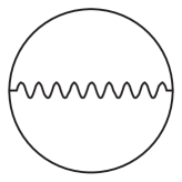
Figure 1: The two-loop diagram needed to evaluate $\Gamma_{2}$.

As in refs. Barducci:1984pr ; Barducci:1987gn , we use the following parametrization for $S$

$$S(p)~{}=~{}iA(p){\hat{p}}~{}+~{}B(p)~{}+~{}i\gamma_{5}C(p)$$ (5)

Then, by working in the Landau gauge, it is possible to show that no renormalization of the wave function is required and also that the Ward identity at this order is satisfied by taking the free quark-gluon vertex and the free gluon propagator. We also consider the so-called rigid case, where the strong coupling $g$ is considered fixed at $p^{2}=M^{2}$, where $M$ is a convenient mass scale to be fixed later. In this way the relation between the scalar and pseudoscalar contribution to $\Sigma$ and the terms $B,~{}C$ in Eq. (5) can be easily inverted, leading to the following expression for the effective action, fully expressed in terms of $\Sigma$ (Barducci:1987gn )

$$\Gamma[\Sigma]=\Gamma_{2}[\Sigma]+\Gamma_{\rm log}[\Sigma]$$ (6)

where, separating $\Sigma=\Sigma_{s}+i\gamma_{5}\Sigma_{p}$

$$\Gamma_{2}[\Sigma]=-\frac{8\Omega_{4}N_{c}\pi^{2}}{3g^{2}C_{2}}\int\frac{d^{4}q}{(2\pi)^{4}}{\rm tr}~{}[\Sigma_{s}(q^{2})\square~{}\Sigma_{s}(q^{2})+\Sigma_{p}(q^{2})\square~{}\Sigma_{p}(q^{2})]$$ (7)

with $\Omega_{4}$ being the four-volume and $C_{2}=4/3$ for $N_{c}=3$ the quadratic Casimir of $SU(3)_{c}$. Besides $M$, also $g$ is a parameter of the model. The one-loop term is

$$\Gamma_{\rm log}[\Sigma]=-{\rm Tr}~{}{\rm log}\left(S_{0}^{-1}-\Sigma\right)=-{\rm Tr}~{}{\rm log}~{}\left[i{\hat{p}}-m-\Sigma_{s}(p^{2})-i\gamma_{5}\Sigma_{p}(p^{2})\right]$$ (8)

where the scalar and pseudoscalar parts of the dynamical variable are matrices in $SU(3)$ flavor space (as well as $m$), related to the scalar and pseudoscalar quark condensates through the following equation

$$\Sigma_{s}(p^{2})+i\gamma_{5}\Sigma_{p}(p^{2})=({s}+i\gamma_{5}{p})~{}f(p^{2})$$ (9)

The function $f(p^{2})$ which contains the momentum dependence of the self-energy will be discussed in a moment. The fields

$$\langle s_{ab}\rangle=-\frac{3C_{2}g^{2}}{4NM^{3}}\langle\bar{\Psi}_{a}\Psi_{b}\rangle$$ (10)

$$\langle p_{ab}\rangle=-\frac{3C_{2}g^{2}}{4NM^{3}}\langle\bar{\Psi}_{a}i\gamma_{5}\Psi_{b}\rangle$$ (11)

will be determined by minimizing the effective action. In Eq. (8), $m$ is the mass matrix in flavor space which is taken diagonal

$$m=\left(\begin{array}[]{ccc}m_{u}&0&0\\ 0&m_{d}&0\\ 0&0&m_{s}\end{array}\right)$$

The function $f(p^{2})$ will be chosen requiring that it goes to a constant for $p\to 0$ and as $1/p^{2}$ (mod log terms) for large values of $p$ as suggested by the OPE expansion. By introducing a dimensionless variable $x^{2}=p^{2}/M^{2}$ we will consider the following family of functions

$$\frac{f_{N}(x^{2})}{M}=\displaystyle{\frac{1+x^{2}+x^{4}+...+x^{2N-2}}{1+x^{2}+x^{4}+...+x^{2N-2}+x^{2N}}}$$ (12)

In the limit $N\to\infty$ we get the function used in Barducci:1984pr ; Barducci:1987gn

$${f(x^{2})\over M}=\theta\left(1-x^{2}\right)~{}+~{}\theta\left(x^{2}-1\right)~{}\displaystyle{{1\over x^{2}}}$$ (13)

Notice that for $x\to 0$ we get

$${f_{N}(x^{2})\over M}\sim 1-x^{2N}+..$$ (14)

Now, let us consider for simplicity the chiral limit and zero chemical potentials. In this case it is simple to get the mass-shell condition from the one loop term in Eq. (8) (see for instance Barducci:1989wi )

$$p^{2}+\langle s\rangle^{2}f^{2}_{N}=0$$ (15)

where $\langle s\rangle$ is the field proportional to the scalar condensate (see Eq. (10)). If we want to recover, at least in the infrared regime, a free particle-like dispersion relation (as for instance happens in four fermion theories), we see from Eqs. (14) and (15) that we need $N\geq 2$. In this paper we will choose $N=2$. Notice that the choice $N=1$ would lead to the following dispersion relation in the limit of small momenta

$$p^{2}(1-2\langle s\rangle^{2})+M^{2}\langle s\rangle^{2}+...=0$$ (16)

This might give rise to problems in the broken phase where the coefficient of $p^{2}$ could become negative. However no difficulties arise for the determination of the critical points where $\langle s\rangle\simeq 0$. On the contrary the equation of state could be affected.

We can thus evaluate explicitly the effective potential

$$V={\Gamma\over\Omega_{4}}$$ (17)

which is UV-finite in the chiral limit, whereas it needs to be properly renormalized in the massive case . We have employed the following normalization condition

$$\frac{\partial V}{\partial(m_{a}\langle\bar{\Psi}_{a}\Psi_{a}\rangle)}\Big{|}_{min}=1$$ (18)

In the chiral limit, this requirement is equivalent to the Adler-Dashen relation (see for instance Barducci:1987gn ). Here we will require the validity of this equation at the values of the quark current masses.
By defining $\alpha_{a}=m_{a}/M$ and

$${\chi}_{a}=-\frac{g^{2}}{3M^{3}}\langle\bar{\Psi}_{a}\Psi_{a}\rangle$$ (19)

the normalization condition, using Eq. (10), can be written as

$$\frac{\partial V_{a}}{\partial(\alpha_{a}\chi_{a})}\Big{|}_{min}=-{3M^{4}\over 2\pi^{2}}c=-{3M^{4}\over g^{2}(M)}$$ (20)

where we have introduced the parameter

$$c\equiv\frac{2\pi^{2}}{g^{2}(M)}$$ (21)

The chemical potential and the temperature dependence are introduced following standard methods Dolan:qd (see for example Barducci:1989wi ). In particular the chemical potential is introduced from the very beginning via the usual substitution $p^{\nu}\rightarrow(p_{0}+i\mu,{\vec{p}})$ in ${\hat{p}}$ appearing in the Dirac operator in Eq.  (8). On the other hand the temperature dependence is introduced by substituting to $p_{0}$ the Matsubara frequency $\omega_{n}=(2n+1)\pi T$ in all the $p_{0}$ dependent terms appearing in the effective action. The reason for this asymmetrical treatment is that the $p$ dependence in the self-energies becomes relevant only at $p\gg M$ whereas, as we shall see we will be interested in chemical potentials lower than $M$.

III Results at finite temperature and density

In order to get the effective action we need to calculate the determinant of the operator appearing in Eq. (8). We set to zero the strange quark chemical potential $\mu_{s}=0$ and define $\mu_{I}=(\mu_{u}-\mu_{d})/2$ and $\mu_{B}=(\mu_{u}+\mu_{d})/2$. The operator is given by the following $3\otimes 3$ matrix in flavor space:

$$\begin{pmatrix}i(\omega_{n}+i\mu_{u})\gamma_{0}+i{\vec{p}}\cdot{\vec{\gamma}}-F_{u}&~{}~{}~{}~{}\rho f_{2}\gamma_{5}&0\cr-\rho f_{2}\gamma_{5}&i(\omega_{n}+i\mu_{d})\gamma_{0}+i{\vec{p}}\cdot{\vec{\gamma}}-F_{d}&0\cr 0&0&i\omega_{n}\gamma_{0}+i{\vec{p}}\cdot{\vec{\gamma}}-F_{s}\end{pmatrix}$$ (22)

where we have defined $F_{a}=m_{a}+f_{2}\chi_{a}$; $~{}a=u,d,s$ and with $f_{2}$ given in Eq. (12) with $N=2$. Also $p^{2}=\omega_{n}^{2}+|\vec{p}\,|^{2}$. Here $\rho$ is related to the charged pion condensate

$$\rho=-\frac{g^{2}}{6M^{3}}(\langle\bar{u}\gamma_{5}d\rangle-\langle\bar{d}\gamma_{5}u\rangle)$$ (23)

We have directly set to zero the hyper-charged condensates in the strange sector, since we do not expect the formation of such condensates for $\mu_{s}=0$. The strange sector thus factorizes and the determination of the phase diagram for approximate chiral symmetry restoration is performed by studying the behavior of the light $\langle{\bar{u}}u\rangle$ and $\langle{\bar{d}}d\rangle$ quark condensates, independently on the strange quark condensate. To evaluate the effective action, we perform the sum over the Matsubara frequencies which solve the mass-shell condition given by the vanishing of the determinant in Eq. (22) using standard methods Dolan:qd . Although formally straightforward, the calculation is a very hard numerical task. Actually, at each integration step on $|{\vec{p}}|$, we have to solve a twentieth order algebraic equation in $\omega_{n}$ in the $u-d$ sector. The part relative to the strange quark is obviously easier to deal with. The coefficients of this equation depend also on the parameters $\chi_{u},\chi_{d},\rho,\mu_{u},\mu_{d},m_{u},m_{d}$.

Before discussing the results at finite density and temperature let us review how we fix the parameters appearing in the effective action. This is done by looking at $T=\mu=0$. The parameters that we have to fit are $c$, $M$, $m_{u}$, $m_{d}$, $m_{s}$. These are obtained by using as input parameters the following physical quantities $m_{\pi^{\pm}}$, $m_{K^{\pm}}$, $m_{K^{0}}$, $f_{\pi}$ and $f_{K}$. The results of the fit are given in Table I, whereas the values of the input experimental quantities, together with the result we get from the fit procedure are given in Table II.

$$\begin{array}[]{|c|c|}\hline\cr{\rm{\bf Parameters}}&{\rm{\bf Fitted~{}Values}}\\ \hline\cr M&529~{}{\rm MeV}\\ \hline\cr c&1.0\\ \hline\cr m_{u}&4.4~{}{\rm MeV}\\ \hline\cr m_{d}&6.2~{}{\rm MeV}\\ \hline\cr m_{s}&110~{}{\rm MeV}\\ \hline\cr\end{array}$$

Table 1: Fit of the parameters.

$$\begin{array}[]{|c|c|c|}\hline\cr{\rm{\bf Input~{}parameters}}&{\rm{\bf Fitted~{}Values}}&{\rm{\bf Experimental~{}Values}}\\ \hline\cr m_{\pi^{\pm}}&139~{}{\rm MeV}&139.6~{}{\rm MeV}\\ \hline\cr m_{K^{\pm}}&494~{}{\rm MeV}&493.7~{}{\rm MeV}\\ \hline\cr m_{K^{0}}&499~{}{\rm MeV}&497.7~{}{\rm MeV}\\ \hline\cr f_{\pi}&92~{}{\rm MeV}&92.4~{}{\rm MeV}\\ \hline\cr f_{K}&105~{}{\rm MeV}&113~{}{\rm MeV}\\ \hline\cr\end{array}$$

Table 2: Comparison between the values of the input parameters as obtained from the fit and the experimental results.

With these values of the parameters, we find that at $T=\mu=0$ the quark condensate in chiral limit has the value

$$\langle{\bar{\psi}}\psi\rangle_{0}=-(248~{}{\rm MeV})^{3}$$ (24)

whereas in the massive case

$$\langle{\bar{u}}u\rangle=-(251~{}{\rm MeV})^{3},~{}~{}~{}\langle{\bar{d}}d\rangle=-(253~{}{\rm MeV})^{3},~{}~{}~{}\langle{\bar{s}}s\rangle=-(305~{}{\rm MeV})^{3}$$ (25)

and, by defining the constituent quark masses a la Politzer Pol

$$M_{const}=\bar{\Sigma}(p^{2}=4M_{const}^{2})$$ (26)

we get

$$M_{s}=385~{}{\rm MeV},\ \ \ \ \ \ \ M_{u,d}=256\ \rm{MeV}$$ (27)

where, here and in the following the light quarks have been taken degenerate with mass ${\hat{m}}=(m_{u}+m_{d})/2=5.3~{}{\rm MeV}$.
From the general study at $T=\mu=0$ and in the chiral limit, one finds also that in order to break the chiral symmetry one must have

$$c<1.37$$ (28)

This condition is satisfied by our choice of parameters.

When $\mu_{I}=0$ it was shown that in the model discussed in Barducci:1989wi there is a tricritical point in the chiral limit. The model we are presenting here is essentially the same model with some slight modifications, as for instance, the choice of the function $f_{2}(x)$. However the tricritical point is still present as it can be seen from Fig. 2 (central line), obtained with the choice of parameters of Table I.

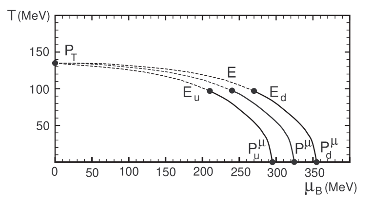
Figure 2: Phase diagram for chiral symmetry in the $(\mu_{B},T)$ plane. For $\mu_{I}=0$ (central line), the cross-over transition line starts from the point $P_{T}=(0,135)$ and ends at the point $E=(240,97)$. The line between $E$ and the point $P^{\mu}=(325,0)$ is the line for the first order transition with discontinuities in the $\langle{\bar{u}}u\rangle$ and $\langle{\bar{d}}d\rangle$ condensates. For $\mu_{I}=30~{}{\rm MeV}$ (side lines), the two cross-over transition lines start from the point $P_{T}=(0,135)$ and end at the points $E_{u}=(210,97)$ and $E_{d}=(270,97)$. The lines between $E_{u}$ and the point $P^{\mu}_{u}=(295,0)$ and between $E_{d}$ and the point $P^{\mu}_{d}=(355,0)$ are the lines for the first order transitions with discontinuities in the $\langle{\bar{u}}u\rangle$ and $\langle{\bar{d}}d\rangle$ condensates respectively.

A complete analysis of the full three parameter space $(\mu_{B},T,\mu_{I})$ has not yet been completed especially in relation with the pion (and hyper-charged) condensate. We have examined the case $T=\mu_{B}=0$ and we have found that there is a phase transition indicated by a finite pion condensate starting at $\mu_{I}=70$ MeV. Since in our model $m_{\pi}\approx 140$ MeV we agree with the results found in the literature Kogut:2002tm ; Kogut:2002zg ; Son:2000xc ; Toublan:1999hx ; Klein:2003fy . We found also that for $m=0$ the critical $\mu_{I}$ is zero. Therefore we will limit our considerations at small isospin chemical potential, say $\mu_{I}=30$ MeV, where we expect the pion condensate $\rho$ to vanish. In this situation the determinant in Eq.  (22) factorizes and the effective action is given by a sum of three independent terms, one for each flavor. Therefore the action is the same as for $\mu_{I}=0$, with each flavor evaluated at its own chemical potential. It follows that the light flavor terms show the same tricritical structure exhibited from the central line in Fig. 2 for $\mu_{I}=0$. Consequently the phase diagram we obtain for a small, fixed isospin chemical potential ($\mu_{I}=30~{}{\rm MeV}$) is described by the two side lines in Fig. 2 with each flavor $u$ and $d$ showing the same structure as the central line but with a split chemical potential $\mu_{u,d}=\mu_{B}\pm\mu_{I}$. Notice also that although the Figure extends up to zero temperature, this part should not be taken too seriously due to the existence of color superconductivity.

IV CONCLUSIONS

In this paper we have discussed an approximate model of QCD (ladder-QCD) at finite temperature and densities. In particular we have considered the experimentally important situation of a non-vanishing isospin chemical potential. This situation has been already explored by various authors previously and we confirm, in particular, the results found in Klein:2003fy and Toublan:2003tt about the splitting of the first order transition line in the plane $(\mu_{B},T)$, for small $\mu_{I}$. As pointed out in Toublan:2003tt this result could be relevant for ion physics since the first order transition line is split symmetrically with respect to the original line at $\mu_{I}=0$. This implies a reduction of the value of the baryon chemical potential at the tricritical point of an amount given by $\mu_{I}$, making easier the possibility of discovering it experimentally. Since it is very difficult to perform first principle analysis of QCD at finite baryon density, we think that it is important to show that certain features as the existence of the tricritical point and the possible splitting of the first order transition line are common to several models. This suggests that these features might possess some universal character. However we should stress that the result of the splitting of the first order transition line is strictly related to the factorization in flavor space. For instance, in the two flavor case, the four-fermi interaction due to the instanton effects leads to a mixing of the flavors that, if sufficiently large, might wash out the mixing. We think that this point needs further analysis in the more complete scheme with three flavors.

References

- (1) K. Rajagopal and F. Wilczek, in At the Frontier of Physics/handbook of QCD, M. Shifman (ed.), World Scientific, Singapore, Vol. 3, p. 2061, [arXiv:hep-ph/0011333].
- (2) A. Barducci, R. Casalbuoni, S. De Curtis, R. Gatto and G. Pettini, Phys. Lett. B 231, 463 (1989); Phys. Rev. D 41, 1610 (1990).
- (3) T. Hatsuda and T. Kunihiro, Phys. Rep. 247, 221 (1994).
- (4) M. A. Halasz, A. D. Jackson, R. E. Shrock, M. A. Stephanov and J. J. Verbaarschot, Phys. Rev. D 58, 096007 (1998) [arXiv:hep-ph/9804290].
- (5) J. Berges and K. Rajagopal, Nucl. Phys. B 538, 215 (1999) [arXiv:hep-ph/9804233].
- (6) P. F. Bedaque, Nucl. Phys. A 697, 569 (2002) [arXiv:hep-ph/9910247].
- (7) M. G. Alford, J. A. Bowers and K. Rajagopal, Phys. Rev. D 63, 074016 (2001) [arXiv:hep-ph/0008208].
- (8) M. Buballa and M. Oertel, Phys. Lett. B 457, 261 (1999) [arXiv:hep-ph/9810529].
- (9) F. Neumann, M. Buballa and M. Oertel, Nucl. Phys. A 714, 481 (2003) [arXiv:hep-ph/0210078].
- (10) A. Steiner, M. Prakash and J. M. Lattimer, Phys. Lett. B 486, 239 (2000) [arXiv:nucl-th/0003066].
- (11) A. W. Steiner, S. Reddy and M. Prakash, Phys. Rev. D 66, 094007 (2002) [arXiv:hep-ph/0205201].
- (12) B. Klein, D. Toublan and J. J. Verbaarschot, arXiv:hep-ph/0301143.
- (13) D. Toublan and J. B. Kogut, arXiv:hep-ph/0301183.
- (14) M. Frank, M. Buballa and M. Oertel, arXiv:hep-ph/0303109.
- (15) Z. Fodor and S. D. Katz, Phys. Lett. B 534, 87 (2002) [arXiv:hep-lat/0104001].
- (16) Z. Fodor and S. D. Katz, JHEP 0203, 014 (2002) [arXiv:hep-lat/0106002].
- (17) J. B. Kogut and D. K. Sinclair, Phys. Rev. D 66, 014508 (2002) [arXiv:hep-lat/0201017].
- (18) J. B. Kogut and D. K. Sinclair, Phys. Rev. D 66, 034505 (2002) [arXiv:hep-lat/0202028].
- (19) D. T. Son and M. A. Stephanov, Phys. Rev. Lett. 86, 592 (2001) [arXiv:hep-ph/0005225].
- (20) D. Toublan and J. J. Verbaarschot, Int. J. Mod. Phys. B 15, 1404 (2001) [arXiv:hep-th/0001110].
- (21) R. Casalbuoni, S. De Curtis, D. Dominici and R. Gatto, Phys. Lett. B 140, 228 (1984); Phys. Lett. B 140, 357 (1984).
- (22) A. Barducci, R. Casalbuoni, S. De Curtis, D. Dominici and R. Gatto, Phys. Lett. B 147, 460 (1984); Phys. Rev. D 38, 238 (1988).
- (23) A. Barducci, R. Casalbuoni, G. Pettini and R. Gatto, Phys. Rev. D 49, 426 (1994).
- (24) R. Jackiw, Phys. Rev. D 9, 1686 (1974).
- (25) J. M. Cornwall, R. Jackiw and E. Tomboulis, Phys. Rev. D 10, 2428 (1974).
- (26) L. Dolan and R. Jackiw, Phys. Rev. D 9, 3320 (1974).
- (27) D. Politzer, Nucl. Phys. B 117, 397 (1976).