Chapter 0 EVENT BY EVENT FLUCTUATIONS

Contents

1. 0 EVENT BY EVENT FLUCTUATIONS
   1. 1 Introduction
   2. 2 Fluctuations in a thermal system
      1. 1 Fluctuations in a grand canonical ensemble
      2. 2 Fluctuations in a canonical ensemble
      3. 3 Phase Transitions and Fluctuations
   3. 3 Other fluctuations
      1. 1 Volume fluctuations
      2. 2 Fluctuation from initial collisions
   4. 4 Fluctuations and Correlations
      1. 1 Correlations and charge fluctuations
      2. 2 Correlations and Balance Function
   5. 5 Observable fluctuations
      1. 1 Fluctuations of Ratios
      2. 2 Fluctuations of the mean energy and mean transverse momentum
      3. 3 Fluctuations of particle ratios
      4. 4 Kaon Fluctuations
   6. 6 Experimental Situation
      1. 1 Fluctuation in elementary collisions
      2. 2 Fluctuations in Heavy Ion Reactions
   7. 7 Conclusions and Outlook

1 Introduction

The study and analysis of fluctuations are an essential method to characterize a physical system. In general, one can distinguish between several classes of fluctuations. On the most fundamental level there are quantum fluctuations, which arise if the specific observable does not commute with the Hamiltonian of the system under consideration. These fluctuations probably play less a role for the physics of heavy ion collisions. Second, there are “dynamical” fluctuations reflecting the dynamics and responses of the system. They help to characterize the properties of the bulk (semi-classical) description of the system. Examples are density fluctuations, which are controlled by the compressibility of the system. Finally, there are “trivial” fluctuations induced by the measurement process itself, such as finite number statistics etc. These need to be understood, controlled and subtracted in order to access the dynamical fluctuations which tell as about the properties of the system.

Fluctuations are also closely related to phase transitions. The well known phenomenon of critical opalescence is a result of fluctuations at all length scales due to a second order phase transition. First order transitions, on the other hand, give rise to bubble formation, i.e. density fluctuations at the extreme. Considering the richness of the QCD phase-diagram as sketched in Fig.1

Figure 1: Schematic picture of the QCD phase-diagram

the study of fluctuations in heavy ions physics should lead to a rich set of phenomena.

The most efficient way to address fluctuations of a system created in a heavy ion collision is via the study of event-by-event (E-by-E) fluctuations, where a given observable is measured on an event-by-event basis and the fluctuations are studied over the ensemble of the events. In most cases (namely when the fluctuations are Gaussian) this analysis is equivalent to the measurement of two particle correlations over the same region of acceptance [12]. Consequently, fluctuations tell us about the 2-point functions of the system, which in turn determine the response of the system to external perturbations.

In the framework of statistical physics, which appears to describe the bulk properties of heavy ion collisions up to RHIC energies, fluctuations measure the susceptibilities of the system. These susceptibilities also determine the response of the system to external forces. For example, by measuring fluctuations of the net electric charge in a given rapidity interval, one obtains information on how this (sub)system would respond to applying an external (static) electric field. In other words, by measuring fluctuations one gains access to the same fundamental properties of the system as “table top” experiments dealing with macroscopic probes. In the later case, of course, fluctuation measurements would be impossible.

In addition, the study of fluctuations may reveal information beyond its thermodynamic properties. If the system expands, fluctuations may be frozen in early and thus tell us about the properties of the system prior to its thermal freeze out. A well known example is the fluctuations in the cosmic microwave background radiation, as first observed by COBE [1].

The field of event-by-event fluctuations is relatively new to heavy ion physics and ideas and approaches are just being developed. So far, most of the analysis has concentrated on transverse momentum and the net charge fluctuations.

Transverse momentum fluctuations should be sensitive to temperature/energy fluctuations [57, 53]. These in turn provide a measure of the heat capacity of the system [44]. Since the QCD phase transition is associated with a maximum of the specific heat, the temperature fluctuations should exhibit a minimum in the excitation function. It has also been argued [55, 56] that these fluctuations may provide a signal for the long range fluctuations associated with the tri-critical point of the QCD phase diagram. In the vicinity of the critical point the transverse momentum fluctuations should increase, leading to a maximum of the fluctuations in the excitation function.

Charge fluctuations [6, 35], on the other hand, are sensitive to the fractional charges carried by the quarks. Therefore, if an equilibrated partonic phase has been reached in these collisions, the charge fluctuations per entropy would be about a factor of 2 to 3 smaller than in an hadronic scenario.

In this review, we will systematically examine the principles and the practices of fluctuations such as the momentum and the charge fluctuations as applied to the heavy ion collisions. In doing so, various concepts of “average” need to be introduced. They are:

• Thermal average

• Event-by-event average as a whole

• Averages over various parts of event-by-event average such as clusters and particles emitted by clusters.

When necessary, we will use subscripts to distinguish these various averages. However whenever it is clear from the context, or if a relation is of a general nature such as the definition of a variance, we will simply use the symbol $\left\langle...\right\rangle$ to denote the average.

The rest of this review is organized as follows. In section 2, we briefly review the basic concepts of thermal fluctuations and its relevance to heavy ion physics. In section 3, we examine possible sources of fluctuations other than the thermal ones and their effect on experimental measurements. In section 4, the relationships between the underlying correlation functions and charge fluctuations and also balance functions are established and their physical meaning made clear. In section 5, various ways of measuring fluctuations proposed so far in literature are briefly reviewed and their inter-relationships established. In section 6, past and current experimental results are examined in the light of the preceding discussions. We conclude in section 7.

We regret that due to the lack of space and also expertise on the authors’ side, such interesting topics as Disoriented Chiral Condensate or Hanbury-Brown-Twiss effects couldn’t be discussed in detail in this review. Also for the same reason, it was impossible for us to cover all the relevant references although we tried our best. If there is any such glaring omission, we apologies to the authors.

2 Fluctuations in a thermal system

To a good approximation the system produced in a high energy heavy ion collision can be considered to be close to thermal equilibrium. Therefore let us first review the properties of fluctuations in a thermal system. Most of this can be found in standard textbooks on statistical physics such as e.g. Ref.[44] and we will only present the essential points here.

Typically one considers a thermal system in the grand-canonical ensemble. This is the most relevant description for heavy ion collisions since usually only a part of the system – typically around mid-rapidity – is considered. Thus energy and conserved quantum numbers may be exchanged with the rest of the system, which serves as a heat-bath. There are, however, important exceptions when the number of conserved quanta is small. In this case an explicit treatment of these conserved charges is required, leading to a canonical description of the system [20] and to significant modifications of the fluctuations, as we shall discuss below. In the following, we first discuss fluctuations based on a grand canonical ensemble and then later point out the differences to a canonical treatment.

1 Fluctuations in a grand canonical ensemble

Assuming we are dealing with a system with one conserved quantum number (such as the electric charge, baryon number etc.) the grand canonical partition function is given by

$$Z=\sum_{\rm states\,\,i}\left\langle i\left|\exp(-\beta(\hat{H}-\mu\hat{Q}))\right|i\right\rangle\equiv{\rm Tr}[\exp(-\beta(\hat{H}-\mu\hat{Q}))]$$ (1)

where $\beta=1/T$ represents the inverse temperature of the system, $Q$ is the conserved charge under consideration and $\mu$ is the corresponding chemical potential. Here the sum covers a complete set of (many particle) states. The relevant free energy $F$ is related to the partition function via

$$F=-T\log Z$$ (2)

We can further introduce the statistical operator

$$\hat{\rho}_{\rm G}\equiv\frac{1}{Z}\exp\left[-\beta(\hat{H}-\mu\hat{Q})\right]=\exp\left[-\beta(\hat{H}-\mu\hat{Q}-F)\right]$$ (3)

and the moments of the grand-canonical distribution:

$$\left\langle X^{n}\right\rangle_{\rm G}\equiv{\rm Tr}[\hat{X}^{n}\,\hat{\rho}_{\rm G}]$$ (4)

For a thermal system, typical fluctuations are Gaussian [44] and are characterized by the variance defined by

$$\left\langle\delta X^{2}\right\rangle\equiv\left\langle X^{2}\right\rangle-\left\langle X\right\rangle^{2}$$ (5)

In the case of grand-canonical ensemble, fluctuations of quantities which characterize the thermal system, such as the energy or the conserved charges, can be expressed in terms of appropriate derivatives of the partition function. Of special interest in the context of heavy ion collisions are energy/temperature fluctuations, which are often related to the fluctuations of the transverse momentum as well as electric charge/baryon number fluctuations.

Fluctuations of the energy and of the conserved charges

As already pointed out at the beginning of this section when analyzing the system created in a heavy ion collisions, one usually studies only a small subsystem around mid-rapidity. In a statistical framework, this situation is best represented by a grand canonical ensemble, where the exchange of conserved quantum number with the rest of the system is taken into account. The equilibrium state is then characterized by the appropriate conjugate variables, namely the temperature and the chemical potentials for the energy and the conserved quantities, respectively.

As a consequence, energy as well as the conserved charges may fluctuate and the size of fluctuations reveals additional properties of the matter, the so called susceptibilities, which also characterize the response of the system to external forces.

For example, the fluctuation of the conserved charge in the subsystem under consideration is given by

$$\left\langle\delta Q^{2}\right\rangle_{\rm G}=T^{2}\frac{\partial^{2}}{\partial\mu^{2}}\log Z=-T\frac{\partial^{2}}{\partial\mu^{2}}F$$ (6)

Similarly, fluctuations of the energy can be expressed in terms of derivatives of the partition function with respect to the temperature

$$\left\langle\delta E^{2}\right\rangle_{\rm G}=\frac{\partial^{2}}{\partial\beta^{2}}\log Z=-T^{3}\frac{\partial^{2}}{\partial T^{2}}F=T^{2}C_{V}$$ (7)

Note that the energy fluctuations are proportional to the heat capacity of the system, $C_{V}$. Thus one would expect that these fluctuations obtain a maximum as the system moves through the QCD phase-transition, which, among others, is characterized by a maximum of the heat capacity.

An alternative way [57, 53] is to study temperature fluctuations in micro-canonical ensemble which are inversely proportional to the heat capacity [44]

$$\left\langle\delta T^{2}\right\rangle_{\rm MC}=\frac{T^{2}}{C_{V}}.$$ (8)

However, for situation at hand, which is best described by a grand canonical ensemble, energy fluctuations appear to be the more appropriate observable.

The second derivatives of the free energy, which characterize the fluctuations, are usually referred to as susceptibilities. Thus we have the charge susceptibility

$$\chi_{Q}=-\frac{1}{V}\frac{\partial^{2}}{\partial\mu^{2}}F$$ (9)

and the “energy susceptibility”

$$\chi_{E}=-\frac{1}{V}\frac{\partial^{2}}{\partial T^{2}}F=\frac{c_{v}}{T}$$ (10)

which is related to the specific heat. And just as the specific heat determines the response of the (sub)system to a change of temperature the charge susceptibility characterizes the response to a change of chemical potential. In case of electric charge, this would be the response to an external electric field.

In thermal field theory these susceptibilities are given by correlation functions of the appropriate operators. For example the charge susceptibility is given by the space-like limit of the static time-time component of the electromagnetic current-current correlator [41, 43, 48, 22]

$$\chi_{Q}=-\Pi_{00}(\omega=0,q\rightarrow 0)$$ (11)

with

$$\Pi_{\mu\nu}(k)=i\int d^{4}x\exp(-ikx)\left\langle\hat{\rho}T^{*}(j_{u}(x)j_{u}(0))\right\rangle$$ (12)

It is interesting to note, that the charge susceptibility is directly proportional to the electric mass [41],

$$m_{\rm el}^{2}=e^{2}\chi_{Q}$$ (13)

Equation Eq. (11) allows to calculate the electric mass in any given model (see e.g. [23, 22, 48, 14, 13]) and in particular in Lattice QCD [30, 26]. Since dilepton and photon production rates are given in terms of the imaginary part of the same current-current correlation function – taken at different values of $\omega$ and $q$ – model calculations for these processes will also give predictions for the charge susceptibility, which then can be compared with lattice QCD results. As shown in [48] an extraction of $\chi_{Q}$ from Dilepton data via dispersion relations, however is not possible. For that one needs also information for the space-like part of $\Pi_{00}$ which is not easily accessible by heavy ion experiments.

Charge fluctuations are of particular interest to heavy ion collisions, since they provide a signature for the existence of a de-confined Quark Gluon Plasma phase [6, 35]. Let us, therefore, discuss charge fluctuations in more detail.

Consider a classical ideal gas of positively and negatively charged particles of charge $\pm q$. The fluctuations of the total charge contained in a subsystem of $N$ particles is then given by

$$\left\langle\delta Q^{2}\right\rangle = q^{2}\left\langle(\delta N_{+}-\delta N_{-})^{2}\right\rangle$$ (14)

$$= q^{2}\left[\left\langle\delta N_{+}^{2}\right\rangle+\left\langle\delta N_{-}^{2}\right\rangle-2\left\langle\delta N_{-}\delta N_{+}\right\rangle\right].$$

Since correlations are absent in an ideal gas, $\left\langle\delta N_{-}\delta N_{+}\right\rangle=0$. Furthermore, for a classical ideal gas,

$$\left\langle\delta N^{2}\right\rangle_{\rm MB}=\left\langle N\right\rangle_{\rm MB}$$ (15)

where the subscript MB stands for Maxwell-Boltzmann. This implies

$$\left\langle\delta Q^{2}\right\rangle_{\rm MB}=q^{2}\left\langle N_{+}+N_{-}\right\rangle_{\rm MB}=q^{2}\left\langle N_{\rm ch}\right\rangle_{\rm MB}$$ (16)

where $N_{\rm ch}=N_{+}+N_{-}$ denotes the total number of charged particles. Taking quantum statistics into account modifies the results somewhat, since the number fluctuations are not Poisson anymore (see e.g. [52])

$$\left\langle\delta N^{2}\right\rangle_{\rm G}=\left\langle N\right\rangle_{\rm G}\left(1\pm\left\langle n_{\pm}\right\rangle_{\rm G}\right)\equiv\omega_{\pm}\left\langle N\right\rangle_{\rm G}.$$ (17)

where

$$\left\langle n_{\pm}\right\rangle_{\rm G}\equiv{\int d^{3}p\,n_{\pm}(p)^{2}\over\int d^{3}p\,n_{\pm}(p)}$$ (18)

Here, $(+)$ refers to Bosons and $(-)$ to Fermions, and $n_{\pm}(p)$ represents the respective single particle distribution functions. For the temperatures and densities reached in heavy ion collisions, however, the corrections due to quantum statistics are small. For a pion gas at temperature $T=170\hbox{\,MeV}$ $\omega_{\pi}=1.13$ [10].

Obviously, charge fluctuations are sensitive to the square of the charges of the particles in the gas. This can be utilized to distinguish a Quark Gluon Plasma, which contains particles of fractional charge, from a hadron gas where the particles carry unit charge. Charge fluctuations per particle should be smaller in a Quark Gluon Plasma than in a hadron gas. The appropriate observable to study is then the charge fluctuations per entropy. To illustrate this point, let us consider a non-interacting pion gas and Quark-Gluon gas in the classical approximation. Corrections due to quantum statistics and due to the presence of resonances are discussed in detail in [6, 35, 34]. In a neutral pion gas the charge fluctuations are due to the charged pions, which are equally abundant

$$\left\langle\delta Q_{\pi}^{2}\right\rangle_{\rm MB}=\left\langle N_{\pi^{+}}\right\rangle_{\rm MB}+\left\langle N_{\pi^{-}}\right\rangle_{\rm MB}$$ (19)

whereas in a Quark Gluon Plasma the quarks and anti-quarks are responsible for the charge fluctuations

$$\left\langle\delta Q^{2}_{q}\right\rangle_{\rm MB}=Q_{u}^{2}\left\langle N_{u}\right\rangle_{\rm MB}+Q_{d}^{2}\left\langle N_{d}\right\rangle_{\rm MB}=\frac{5}{9}\left\langle N_{q}\right\rangle_{\rm MB}$$ (20)

where $N_{q}=N_{u}=N_{d}$ denotes the number of quarks and anti-quarks. For a classical ideal gas of massless particles the entropy is given by

$$S_{\rm MB}=4\left\langle N\right\rangle_{\rm MB}$$ (21)

For a pion gas, this yields

$$S_{\pi}=4\left(\left\langle N_{\pi^{+}}\right\rangle_{\rm MB}+\left\langle N_{\pi^{-}}\right\rangle_{\rm MB}+\left\langle N_{\pi^{0}}\right\rangle_{\rm MB}\right)$$ (22)

and for a Quark Gluon Plasma

$$S_{\rm QGP} = 4\left(\left\langle N_{u}\right\rangle_{\rm MB}+\left\langle N_{d}\right\rangle_{\rm MB}+\left\langle N_{g}\right\rangle_{\rm MB}\right)$$ (23)

$$= 4\left(2\left\langle N_{q}\right\rangle_{\rm MB}+\left\langle N_{g}\right\rangle_{\rm MB}\right)$$

where $N_{g}$ denotes the number of gluons. Therefore, the ratio of charge fluctuation per entropy in a pion gas is

$$\frac{\left\langle\delta Q_{\pi}^{2}\right\rangle_{\rm MB}}{S_{\pi}}=\frac{1}{6}$$ (24)

whereas for a 2-flavor Quark Gluon Plasma it is

$$\frac{\left\langle\delta Q_{q}^{2}\right\rangle_{\rm MB}}{S_{\rm QGP}}=\frac{1}{24}$$ (25)

Consequently, the charge fluctuations per degree of freedom in a Quark Gluon Plasma are a factor of four smaller than that in a pion gas. Hadronic resonances, which constitute a considerable fraction of a hadron gas reduce the result for the pion gas by about 30 % [35, 34], leaving still a factor 3 signal for the existence of the Quark Gluon Plasma.

The above ratio, $\left\langle\delta Q^{2}\right\rangle/S$ can also be calculated using lattice QCD [30]. Above the critical temperature, the value obtained from lattice agree rather well with that obtained in our simple Quark Gluon Plasma model here [35]. More recent calculations for the charge susceptibility [26] give a somewhat smaller value, which would make the observable even more suitable.

Unfortunately, at present lattice results are not available for this ratio below the critical temperature. Here one has to resort to hadronic model calculations. This has been done in [22, 23] using either a virial expansion, a chiral low energy expansion or an explicit diagrammatic calculation. In all cases, the ratio is slightly increased due to interactions, thus enhancing the signal for the Quark Gluon Plasma.

2 Fluctuations in a canonical ensemble

As pointed out in the beginning of this section, once the number of conserved quanta is small, i.e. of the order of one per event, the grand canonical treatment, where charges are conserved only on the average, is not adequate anymore. Instead the description needs to ensure that the quantum number is conserved explicitly in each event. Since the deposited energy is still large and is distributed over many degrees of freedom, the canonical ensemble is the ensemble of choice.

Obviously the fluctuations of the energy is identical to the grand canonical ensemble, but fluctuations of particles which carry the conserved charge are affected. As an example, let us consider the fluctuations of Kaons in low energy heavy ion collisions. At 1-2 AGeV bombarding energy, only very few kaons are being produced $\left\langle N_{K}\right\rangle\simeq 0.1$ [58], which makes an explicit treatment of strangeness conservation necessary. For simplicity, let us consider Kaons and Lambdas/Sigmas as the only particles carrying strangeness. In the canonical ensemble, where strangeness is conserved explicitly, the partition function is given by[20]

$$Z_{\rm C}=Z^{0}_{\rm rest}\sum_{n=0}^{\infty}\frac{1}{n!^{2}}\left(Z^{0}_{K}Z^{0}_{\Lambda}\right)^{n}$$ (26)

where $Z^{0}_{\rm rest}$ is the standard (grand canonical) partition for all the other non strange particles and $Z^{0}_{K}$ , $Z^{0}_{\Lambda}$ are the single particle partition functions for Kaons and Lambdas, respectively. In the classical limit, these are given by

$$Z^{0}_{K} = 2V\int\frac{d^{3}p}{(2\pi)^{3}}\exp(-\beta E_{K})=\left\langle N^{0}_{K}\right\rangle_{\rm MB}\$$ (27)

$$Z^{0}_{\Lambda} = 4V\int\frac{d^{3}p}{(2\pi)^{3}}\exp(-\beta(E_{\Lambda}-\mu_{B}))=\left\langle N^{0}_{\Lambda}\right\rangle_{\rm MB}$$ (28)

Here, the degeneracy factor of $d=2,4$ for Kaons and Lambdas, respectively, take into account the presence of the $K^{0}$ and $\Sigma$ particles. Note that $Z^{0}$ is simply the number of particles in the grand canonical ensemble in the limit of vanishing strange chemical potential. Given the above partition function, the probability $P_{n}$ to find $n$ “Kaons” is given by [42, 36, 45]

$$P_{n}=\frac{\epsilon^{n}}{I_{0}(2\sqrt{\epsilon})(n!)^{2}}$$ (29)

where $I_{0}$ is the modified Bessel function and

$$\epsilon=Z^{0}_{K}Z^{0}_{\Lambda}=\left\langle N^{0}_{K}\right\rangle_{\rm MB}\left\langle N^{0}_{\Lambda}\right\rangle_{\rm MB}$$ (30)

Given the probabilities Eq. (29), one can easily calculate the canonical ensemble average

$$\left\langle N_{K}\right\rangle_{\rm C} = \sqrt{\epsilon}\frac{I_{1}(2\sqrt{\epsilon})}{I_{0}(2\sqrt{\epsilon})}=\epsilon-\frac{\epsilon^{2}}{2}+\frac{\epsilon^{3}}{6}+\ldots$$

$$\left\langle N_{K}^{2}\right\rangle_{\rm C} = \epsilon$$ (31)

so that the second factorial moment

$$F_{2}^{\rm C}\equiv\frac{\left\langle N(N-1)\right\rangle_{\rm C}}{\left\langle N\right\rangle_{\rm C}^{2}}=\frac{1}{2}+\frac{\epsilon}{6}+\ldots=\frac{1}{2}+\frac{\left\langle N_{K}\right\rangle_{\rm C}}{6}+\ldots$$ (32)

This is to be contrasted with the grand canonical result, which follows in the limit of $\epsilon\gg 1$. In this case,

$$\left\langle N^{2}\right\rangle_{\rm G}-\left\langle N\right\rangle_{\rm G}=\left\langle N\right\rangle_{\rm G}^{2}$$ (33)

so that

$$F_{2}^{\rm G}=1$$ (34)

Thus for $\left\langle N\right\rangle\ll 1$ the effect of explicit strangeness conservation reduces the second factorial moment by almost a factor of two. This suppression of the factorial moment due to explicit charge conservation can be utilized to measure the degree of equilibration reached in these collisions (see section 5).

3 Phase Transitions and Fluctuations

As already mentioned in the introduction, the QCD phase diagram is expected to be rich in structure. Besides the well known and much studied transition at zero chemical potential, which is most likely a cross over transition, a true first order transition is expected at finite quark number chemical potential. It has been argued [55] that the phase separation line ranges from zero temperature and large chemical potential to finite temperature and smaller chemical potential where it ends in a critical end-point $(E)$ (see Fig.1). Here the transition is of second order. There is also a first attempt to determine the position of the critical point in Lattice QCD [25].

As discussed in [55], the associated massless mode carries the quantum numbers of $\sigma$-meson, i.e. scalar iso-scalar, whereas the pions remain massive due to explicit chiral symmetry breaking as a result of finite current quark masses.

Fluctuations are a well known phenomenon in the context of phase transitions. In particular, second order phase transitions are accompanied by fluctuations of the order parameter at all length scales, leading to phenomena such as critical opalescence [44]. However, since the system generated in a heavy ion collision expands rather rapidly, critical slowing down, another phenomenon associated with a second order phase transition, will prevent the long wavelength modes to fully develop. In Ref.[9] these competing effects have been estimated and authors arrive at a maximum correlation length of about $\xi\simeq 3\hbox{\,fm}$ if the system passes through the critical (end) point of the QCD phase diagram.

In Ref.[56] the authors argue that if the system freezes out close to the critical end-point, the long range correlations introduced by the massless $\sigma$-modes lead to large fluctuations in the pion number at small transverse momenta. In the thermodynamic limit, this fluctuations would diverge, but in a realistic scenario, where the long wavelength modes do not have time to fully develop, the fluctuations are limited by the correlation length. In Ref.[9] it is estimated that a correlation length of $\xi\simeq 3\hbox{\,fm}$ will result in $\sim 5-10\%$ increase in fluctuations of the mean transverse momentum, which should be observable with present day large acceptance detectors such as STAR and NA49. Since the precise position of the critical point is not well known, what is needed is a measurement of the excitation function of these fluctuations.

If the system undergoes a first order phase transition, bubble formation may occur. Since each bubble is expected to decay in many particles this leads to large multiplicity fluctuations in a given rapidity interval [8, 32]. Fluctuations of particle ratios, on the other hand, should be reduced due to the correlations induced by bubble formation[34].

3 Other fluctuations

In heavy ion collisions, there are many sources of non-statistical fluctuations. To extract physically interesting information from the observed fluctuations, it is crucial that we know the sizes of these other fluctuations. In this section, we discuss the geometrical volume fluctuations and fluctuations coming purely from the initial reactions without further rescatterings within the context of wounded nucleon model[8].

1 Volume fluctuations

In heavy ion collisions, we have no real control over the impact parameter of each collision. This implies that geometric fluctuation is unavoidable in the fluctuations of any extensive quantities such as the particle multiplicity and energy. Furthermore, since the system created by a heavy ion collision is finite, one must also consider the thermal fluctuation of the reaction volume[44].

To be more specific, consider the multiplicity $N$. Writing

$$N=\rho V$$ (35)

where $\rho$ is the density and $V$ is the volume, the fluctuation of $N$ can be written as

$$\left\langle\delta N^{2}\right\rangle_{\rm ebe}=\left\langle\delta\rho^{2}\right\rangle_{\rm ebe}\left\langle V\right\rangle_{\rm ebe}^{2}+\left\langle\rho\right\rangle_{\rm ebe}^{2}\left\langle\delta V\right\rangle_{\rm ebe}^{2}$$ (36)

where the subscript ‘ebe’ indicates the event-by-event average measured in an experiment. Normally, what we are interested in are the fluctuations in the thermodynamic limit. In other words, we are only interested in the fluctuation of the density, $\left\langle\delta\rho^{2}\right\rangle$. The second term containing $\left\langle\delta V^{2}\right\rangle$ is therefore undesirable.

To make a rough estimate of the volume fluctuation effect, we first decompose

$$\left\langle\delta V^{2}\right\rangle_{\rm ebe}=\left\langle\delta V^{2}\right\rangle_{\rm th}+\left\langle\delta V^{2}\right\rangle_{\rm geom}$$ (37)

Assume the ideal gas law $PV=NT$ and using

$$\left\langle\delta V^{2}\right\rangle_{\rm th}=-T\left(\partial V\over\partial P\right)_{T}$$ (38)

(see [44]) the thermodynamic volume fluctuation can be estimated as

$$\left\langle\delta V^{2}\right\rangle_{\rm th}=\left\langle V\right\rangle^{2}/\left\langle N\right\rangle_{\rm th}=\left\langle V\right\rangle/\left\langle\rho\right\rangle_{\rm th}$$ (39)

or

$$\left\langle\rho\right\rangle_{\rm th}^{2}\left\langle\delta V\right\rangle^{2}_{\rm th}=\left\langle N\right\rangle_{\rm th}$$ (40)

which is at least as big as the fluctuation due to the thermal density fluctuation (c.f. Eq.(17)).

On top of this, we have purely geometrical fluctuation due to the impact parameter variation. To have an estimate, let us simplify the nucleus as a cylinder with a radius $R$ and the length $L$. Assuming geometrically random choice of impact parameters, one can show that

$${\left\langle\delta V^{2}\right\rangle_{\rm geom}\over\left\langle V\right\rangle_{\rm geom}^{2}}={\frac{2\,{{{b_{\rm max}}}^{2}}}{9\,{{\pi}^{2}}\,{R^{2}}}}+{\frac{16\,{{{b_{\rm max}}}^{3}}}{27\,{{\pi}^{3}}\,{R^{3}}}}+O(b_{\rm max}^{4}/R^{4})$$ (41)

if the impact parameter varies between $b=0$ and $b=b_{\rm max}$. The expansion is of course valid when $b_{\rm max}\ll R$.

As an example, consider 6 % most central collision of two gold ions. For a gold ion, $R\approx 7\,\hbox{\,fm}$ and 6 % corresponds to $b_{\rm max}\approx 3.0\,\hbox{\,fm}$. Plugging in these values to the above formula yields,

$$\left\langle\delta V^{2}\right\rangle_{\rm geom}\approx\left\langle V\right\rangle_{\rm geom}^{2}/170$$ (42)

or

$$\left\langle\rho\right\rangle^{2}\left\langle\delta V^{2}\right\rangle_{\rm geom}=\left\langle N\right\rangle^{2}/170$$ (43)

For $\left\langle N\right\rangle>170$ then, the observed multiplicity fluctuation can be overwhelmingly due to the impact parameter variation.

This difficulty can be circumvented if the average of the fluctuating quantity, say the electric charge $Q$, is zero or close to it. This can be readily seen if one writes

$$\delta Q=\delta q\left\langle V\right\rangle_{\rm ebe}+\left\langle q\right\rangle_{\rm ebe}\delta V$$ (44)

ignoring terms quadratic in $\delta q$ and $\delta V$. Squaring and averaging yield

$$\left\langle\delta Q^{2}\right\rangle_{\rm ebe}=\left\langle\delta q^{2}\right\rangle_{\rm ebe}\left\langle V\right\rangle^{2}+\left\langle\delta V^{2}\right\rangle_{\rm ebe}\left\langle q\right\rangle_{\rm ebe}^{2}$$ (45)

assuming that the fluctuations in the charge density $q$ and the volume $V$ are independent. Usually, $\left\langle\delta q^{2}\right\rangle\sim\left\langle N\right\rangle/\left\langle V\right\rangle^{2}$ and from the above impact parameter consideration, $\left\langle\delta V^{2}\right\rangle=\left\langle V\right\rangle^{2}/C$ where $C=O(100)$.

Therefore, the second term is negligible if

$$\left\langle\delta V^{2}\right\rangle_{\rm ebe}\left\langle q\right\rangle_{\rm ebe}^{2}=\left\langle Q\right\rangle_{\rm ebe}^{2}/C\ll\left\langle N\right\rangle_{\rm ebe}$$ (46)

or

$$\left\langle Q\right\rangle_{\rm ebe}^{2}/\left\langle N\right\rangle_{\rm ebe}\ll C$$ (47)

The STAR detector at RHIC counts about 600 charged particles per unit rapidity in central collisions and $\left\langle Q\right\rangle_{\rm ebe}/\left\langle N\right\rangle_{\rm ebe}\approx 0.1$. In that case,

$$\left\langle Q\right\rangle_{\rm ebe}^{2}/\left\langle N\right\rangle_{\rm ebe}\approx(0.1)^{2}\times 600=6$$ (48)

which is much smaller than $C=O(100)$. If one is to talk about gross features, such error would not matter much. However, if a precision measurement is required, this has to be taken into account.

2 Fluctuation from initial collisions

One of the important issues in heavy ion collisions is that of thermalization. Seemingly ‘thermal’ behaviors of particle spectra are very common in particle/nucleus collision experiments including $e^{+}e^{-}$ collisions and $pp$, $p\bar{p}$ collisions where one would not expect thermalization among secondary particles to occur. This seemingly ‘thermal’ feature results from the way an elementary collision distributes the collision energy among its secondary particles. Mathematically speaking, this is analogous to passing from the micro-canonical ensemble of free particles to the canonical ensemble of free particles. By doing so, one incurs an error. However as the size of the system grows the error becomes negligible.

A way to distinguish simple equi-partition of energy from true thermalization through multiple scatterings is to consider not only the average values but also the fluctuations. For instance, as explained in section 2, the fluctuations of charged multiplicity in thermal system is Poisson or

$$\left\langle\delta N_{\rm ch}^{2}\right\rangle_{\rm MB}=\left\langle N_{\rm ch}\right\rangle_{\rm MB}$$ (49)

However, we do know that in elementary collisions such as $pp$ or $p\bar{p}$, the fluctuation is much stronger due to KNO scaling

$$\left\langle\delta N_{\rm ch}^{2}\right\rangle_{\rm ebe}\propto\left\langle N_{\rm ch}\right\rangle_{\rm ebe}^{2}$$ (50)

Questions then arise: How would $\left\langle\delta N_{\rm ch}^{2}\right\rangle_{\rm ebe}$ behave if there is no scatterings among the secondaries? Will it resemble the thermal case or retain the features of KNO scaling? If it turned out to resemble thermal case, how can we distinguish?

To answer these questions, let us invoke the wounded nucleon model as explained in Ref.[8]. In this model, the final charged particle multiplicity is given by

$$N_{\rm ch}=\sum_{i=1}^{N_{p}}n_{i}$$ (51)

where $N_{p}$ is the number of participating nucleons (participants) in the given event and $n_{i}$ is the number of charged particles from each of the participants. The assumption here is that the production of charged particles from each nucleon is independent and the produced particles do not interact further. In that case, it is not hard to show

$$\left\langle N_{\rm ch}\right\rangle_{\rm ebe}=\left\langle N_{p}\right\rangle_{\rm ebe}\left\langle n\right\rangle_{\rm N}$$ (52)

and

$${\left\langle\delta N^{2}_{\rm ch}\right\rangle_{\rm ebe}\over\left\langle N_{\rm ch}\right\rangle_{\rm ebe}}={\left\langle\delta N_{p}\right\rangle_{\rm ebe}^{2}\over\left\langle N_{p}\right\rangle_{\rm ebe}}\left\langle n\right\rangle_{\rm N}+{\left\langle\delta n^{2}\right\rangle_{\rm N}\over\left\langle n\right\rangle_{\rm N}}$$ (53)

Here $\left\langle...\right\rangle_{\rm N}$ denotes that this average is taken with respect to a single nucleon. It is independent of the system size. Therefore the second term is where KNO makes its appearance. It states that that $\left\langle\delta n^{2}\right\rangle_{\rm N}=c_{\rm KNO}\left\langle n\right\rangle_{\rm N}^{2}$ with $c_{\rm KNO}\approx 0.35$ for proton-proton collisions (for instance, see Ref.[33]). In Ref.[7], it is argued that since nucleons inside a nucleus are tightly correlated, the probability to have all nucleons in the reaction volume participate is very high. Therefore $\left\langle\delta N_{p}^{2}\right\rangle_{\rm ebe}/\left\langle N_{p}\right\rangle_{\rm ebe}$ should be small and ${\left\langle\delta N^{2}_{\rm ch}\right\rangle/\left\langle N_{\rm ch}\right\rangle}=O(\left\langle n\right\rangle_{\rm N})$ which grows with the collision energy.

To compare with a typical heavy ion experiment, however, two more effects need to be considered in addition. First, although the fluctuation of the number of participants due to the nuclear wavefunction is small, geometrical fluctuations due to the variation of impact parameter can introduce more substantial fluctuations in $N_{p}$. Second, a heavy ion experiment usually can observe only a portion of the whole phase space. Therefore when calculating $\left\langle n\right\rangle$ and $\left\langle n^{2}\right\rangle$ we must fold in a binary distribution with $p=\left\langle n\right\rangle_{\rm\Delta\eta}/\left\langle n\right\rangle_{\rm full}$ where $\Delta\eta$ is the detector window. This implies replacing

$$\left\langle n\right\rangle_{\rm N}\to p\left\langle n\right\rangle{N},$$ (54)

$$\left\langle\delta n^{2}\right\rangle_{\rm N}\to(1-p)p\left\langle n\right\rangle_{\rm N}+p^{2}\left\langle\delta n^{2}\right\rangle_{\rm N},$$ (55)

and (56)

$$\left\langle\delta N_{p}^{2}\right\rangle_{\rm ebe}\to\left\langle\delta N_{p}^{2}\right\rangle_{\rm geom}$$

The fluctuation due to the impact parameter variation was estimated in the previous section. Putting everything together then yields

$$\omega_{\rm WNM}\equiv{\left\langle\delta N^{2}_{\rm ch}\right\rangle_{\rm ebe}\over\left\langle N_{\rm ch}\right\rangle_{\rm ebe}}=\left\langle N_{\rm ch}\right\rangle_{\rm geom}\left({\frac{2\,{{{b_{\rm max}}}^{2}}}{9\,{{\pi}^{2}}\,{R^{2}}}}\right)+(1-p)+p\,c_{\rm KNO}\left\langle n\right\rangle_{\rm N}$$

(57)

Here we assumed that tight correlations renders intrinsic participant fluctuation very small and also used the fact that $\left\langle N_{\rm ch}\right\rangle_{\rm geom}=p\left\langle N_{p}\right\rangle_{\rm geom}\left\langle n\right\rangle_{\rm N}$.

A few conclusion can be drawn from Eq.(57). First, if $p$ is sufficiently small or if the observational window is sufficiently small compared to the whole phase space, the fluctuation of the number of charged particle is Poisson. However, this has nothing to do with dynamics. Second, if $p$ is sufficiently large, then $\omega_{\rm WNM}$ becomes significantly larger than 1 since $c_{\rm KNO}\left\langle n\right\rangle_{\rm N}$ is about $7$ at RHIC energy. Third, the ratio $\omega_{\rm WNM}$ depends linearly on $p$. The first point is purely statistical in nature. The second and third points can be used to test the validity of this model where no secondary scattering occurs.

What would change in this consideration if thermalization through multiple scatterings occurs? Suppose that the total number of produced particles is still governed by Eq.(51). In other words, only elastic scatterings happened to the secondary particles. Further suppose $\left\langle\delta n^{2}\right\rangle_{\rm N}$ is still given by the KNO scaling result. In this case, the fluctuations of $N_{\rm ch}$ in the full phase space must remain the same as before and Eq.(53) remains valid. Since binary process does not really care about clusters in this case, Eq.(57) also stays valid. Therefore elastic scatterings alone cannot make any difference in multiplicity fluctuations.

Now let us relax the condition and allow inelastic collisions among the secondaries. The essential role of inelastic collisions is to convert energy into multiplicity and vice versa. Consider a set of events with the same number of participants and same amount of energy deposit. According to Eq.(53), the number of initially produced particles (we will call them ‘initial particles’) have a distribution that is much wider than the Poisson distribution if $\left\langle n\right\rangle_{\rm N}\gg 1$. This wide distribution implies that the distribution of energy per initial particle also has a wide distribution. As argued above, elastic collisions cannot change this situation. If inelastic collisions are allowed, then an event with smaller number of initial particles would tend to produce more particles since collisions in this event have more available energy. In this way, energy is re-distributed evenly and the the multiplicity distribution gets narrower. This is, of course, the process of equi-partition which lies at the heart of thermalization. Therefore if thermalization does occur starting from a certain energy or a certain centrality, $\omega_{N_{\rm ch}}$ must show a corresponding behavior changing from approximately $\left\langle n\right\rangle_{\rm N}>1$ to lower values close to 1 as the energy goes higher or collisions get more central.

4 Fluctuations and Correlations

Fluctuations measure the width of the two particle densities[12] and therefore provides additional information than just the averages. To illustrate this point, let us consider a variable $x(p)$ which depends on momentum of one particle but does not depend on the multiplicity in each event. Let us further consider a generic observable in a given event

$$S(x)=\sum_{i=1}^{N}x(p_{i})\equiv\sum_{i=1}^{N}x(i)$$ (58)

where $N$ is the multiplicity of the event. Since $x(p)$ does not depend on $N$, $S$ is an extensive quantity.

The event averaged moments of this quantity can be expressed as

$$\left\langle S^{k}\right\rangle_{\rm ebe}=\frac{1}{M}\sum_{m=1}^{M}\sum_{i_{1}=1}^{N_{m}}...\sum_{i_{k}=1}^{N_{m}}x_{m}(i_{1})...x_{m}(i_{k})$$ (59)

where $m$ labels the different events and $M$ is their total number. $N_{m}$ is the multiplicity of the event labeled by $m$.

On the other hand, the moments of an extensive quantity $x(p)$ calculated from n-particle inclusive distribution $\rho_{n}(p_{1},...,p_{n})$ are defined as

$$\int dp_{1}...dp_{n}\rho_{n}(p_{1},...,p_{n})[x(p_{1})]^{k_{1}}...[x(p_{n})]^{k_{n}}=$$

$$\frac{1}{M}\sum_{m=1}^{M}\sum_{i_{1}=1}^{N_{m}}...\sum_{i_{n}=1}^{N_{m}}[x_{m}(i_{1})]^{k_{1}}...[x_{m}(i_{n})]^{k_{n}}$$ (60)

where the sums over $i_{1}...i_{n}$ include only the terms for which all indices $i_{1}...i_{n}$ are different from each other.

One sees immediately that (59) and (60) are related.

$$\left\langle S\right\rangle_{\rm ebe}=\int dp\rho_{1}(p)x(p)$$ (61)

$$\left\langle S^{2}\right\rangle_{\rm ebe}=\int dp_{1}dp_{2}\rho_{2}(p_{1},p_{2})\,x(p_{1})x(p_{2})+\int dp\rho_{1}(p)\,[x(p)]^{2}$$ (62)

$$\left\langle S^{3}\right\rangle_{\rm ebe} = \int dp_{1}dp_{2}dp_{3}\rho_{3}(p_{1},p_{2},p_{3})\,x(p_{1})x(p_{2})x(p_{3})$$ (63)

$$\mbox{}+3\int dp_{1}dp_{2}\rho_{2}(p_{1},p_{2})\,x(p_{1})[x(p_{2})]^{2}$$

$$\mbox{}+\int dp\rho_{1}(p)\,[x(p)]^{3}$$

Similar formulas can be derived for higher moments of $S$. By setting $x(p)=1$, one can also find that the integral over $\rho_{n}$ gives the $n$-th factorial moments

$$\int dp_{1}...dp_{n}\,\rho_{n}(p_{1},...,p_{n})=\left\langle N(N-1)\cdots(N-n+1)\right\rangle_{\rm ebe}$$ (64)

We have thus established the relation between inclusive measurements and event-by-event fluctuations for single particle observables [27], such as e.g. the total transverse momentum, particle abundances [28] etc.

For observables concerning different species of particles, we define

$$S_{\alpha}(x)=\sum_{i=1}^{N}x(p_{i})\delta_{\alpha i}$$ (65)

where the $\delta$-function picks out the right species from $N$ particles in the event. The event average $\left\langle S_{\alpha}\right\rangle_{\rm ebe}$ is just as before with the replacement of $\rho_{1}(p)\to\rho_{\alpha}(p)$ and $\int dp\rho_{\alpha}(p)=\left\langle N_{\alpha}\right\rangle_{\rm ebe}$. The average number of pairs is then given by

$$\left\langle S_{\alpha}(x)S_{\beta}(x)\right\rangle_{\rm ebe}={1\over M}\sum_{i=1}^{N_{m}}\sum_{j=1}^{N_{m}}x(p_{i})x(p_{j})\,\delta_{\beta j}\delta_{\alpha i}$$ (66)

In terms of the correlation function, this can be rewritten as

$$\left\langle S_{\alpha}(x)S_{\beta}(x)\right\rangle_{\rm ebe} = \int dp_{\alpha}dp_{\beta}\,\rho_{\alpha\beta}(p_{\alpha},p_{\beta})x(p_{\alpha})x(p_{\beta})$$ (67)

Again by setting $x(p)=1$, one also obtains

$$\int dp_{\alpha}dp_{\beta}\,\rho_{\alpha\beta}(p_{\alpha},p_{\beta})=\left\langle N_{\alpha}N_{\beta}\right\rangle_{\rm ebe}$$ (68)

Similar arguments can be constructed for variables which depend on two or more particle momenta, such as e.g. the fluctuations of Hanburry-Brown Twiss (HBT) two particle correlations. belong to this class. They are of practical interest and will be investigated in heavy ion experiments. Here we will restrict the argument to two particles but it can be readily extended to multiparticle correlations. The details are given in [12].

To summarize, E-by-E fluctuations of any (multiparticle) observable can be re-expressed in terms of inclusive multiparticle distribution. In case of Gaussian fluctuations the multiparticle distributions need to be known up to twice the order of the observable under consideration.

Following these straightforward considerations, it is natural to discuss fluctuations in terms of two particle densities, or equivalently in terms of two particle correlations functions [37, 49]

$$C_{\alpha\beta}(p_{1},p_{2})\equiv\rho_{\alpha\beta}(p_{1},p_{2})-\rho_{\alpha}(p_{2})\rho_{\beta}(p_{1})$$ (69)

Here the labels $\alpha$ and $\beta$ denote general particle properties including different quantum numbers. Thus correlations between different particle types can also be discussed in the same framework.

Instead of the correlation function $C$ often the reduced correlation function

$$R_{\alpha\beta}(p_{1},p_{2})\equiv\frac{C_{\alpha\beta}(p_{1},p_{2})}{\rho_{\alpha}(p_{1})\rho_{\beta}(p_{2})}=\frac{\rho_{\alpha\beta}(p_{1},p_{2})}{\rho_{\alpha}(p_{1})\rho_{\beta}(p_{2})}-1$$ (70)

is used. The advantage of using $R_{\alpha\beta}$ over $C_{\alpha\beta}$ is that the trivial scaling with the square of the number of particles is removed and, therefore, the true strength of the correlations is exposed more transparently. In particular, as shown in Ref.[49], the observable $R_{\alpha\beta}$ has the advantage that it is robust, i.e. it is independent of the detector efficiencies to leading order. Also, the analysis of elementary reactions such as proton-proton has traditionally been done based on the reduced correlation function $R_{\alpha\beta}$ [61] (see also section 1).

In some cases, such as the charge fluctuations (c.f. 1), the fluctuations of the number of particles in a given region of momentum space is considered. In this case one deals with the integrated quantities

$$\left\langle N_{\alpha}\right\rangle_{\Delta\eta} = \int_{\Delta\eta}dp_{\alpha}\rho_{1}(p_{\alpha})$$ (71)

$$\left\langle N_{\alpha}N_{\beta}\right\rangle_{\Delta\eta}-\delta_{\alpha\beta}\left\langle N_{\alpha}\right\rangle_{\Delta\eta} = \int_{\Delta\eta}dp_{\alpha}dp_{\beta}\rho_{2}(p_{\alpha},p_{\beta})$$ (72)

where the notation $\left\langle\ldots\right\rangle_{\Delta\eta}$ is always to be understood as the event-by-event average in a given momentum space region $\Delta\eta$

$$\left\langle S\right\rangle_{\Delta\eta}={1\over M}\sum_{i=1}^{N_{m}}\,x(p)\,\theta(p\in\Delta\eta)$$ (73)

where $\theta(p\in\Delta\eta)=1$ if $p$ falls inside $\Delta\eta$ and zero otherwise. The correlations are then expressed in terms of the ‘robust covariances’[49]

$$\bar{R}_{\alpha\beta} \equiv \frac{\left\langle N_{\alpha}N_{\beta}\right\rangle_{\Delta\eta}-\left\langle N_{\alpha}\right\rangle_{\Delta\eta}\delta_{\alpha\beta}-\left\langle N_{\alpha}\right\rangle_{\Delta\eta}\left\langle N_{\beta}\right\rangle_{\Delta\eta}}{\left\langle N_{\alpha}\right\rangle_{\Delta\eta}\left\langle N_{\beta}\right\rangle_{\Delta\eta}}$$ (74)

$$= \frac{\int_{\Delta\eta}dp_{1}dp_{2}\rho_{\alpha\beta}(p_{1},p_{2})}{\int_{\Delta\eta}dp_{1}\rho_{\alpha}(p_{1})\int_{\Delta\eta}dp_{2}\rho_{\beta}(p_{2})}-1$$

which shares the same virtue as $R_{\alpha\beta}$.

1 Correlations and charge fluctuations

We will now concentrate on charge fluctuations to illustrate the above general considerations. Here we will mainly work out the relationship between the charge fluctuations and the charged particle correlation functions. In full phase space, a conserved charge does not fluctuate, or $\left\langle\delta Q^{2}\right\rangle_{\rm full}=0$. What we are interested in is, however, fluctuations of the net charge in a small phase space window where the effect of this overall charge conservation is small. At the same time, this window should be big enough in order not to lose information on the widths of the correlation functions.

From previous section 1, we know that if a QGP forms, the charge fluctuation per entropy becomes a factor of 2 to 3 smaller than that of the hadronic gas. What we are interested in this section is how that is related to the properties of the charge correlation functions. Since the net charge is $Q=N_{+}-N_{-}$, the variance is

$$\left\langle\delta Q^{2}\right\rangle_{\Delta\eta}=\left\langle\delta N_{+}^{2}\right\rangle_{\Delta\eta}+\left\langle\delta N_{-}^{2}\right\rangle_{\Delta\eta}-2\left\langle\delta N_{+}\,\delta N_{-}\right\rangle_{\Delta\eta}$$ (75)

Written this way, it is clear that to have a small charge fluctuation, we must have a positive correlation between the unlike-sign pairs and it must have enough strength to compensate the independent fluctuations of $N_{\pm}$. The purpose of this section is to elaborate on these points.

To write the charge fluctuations using the correlation functions, we first decompose

$$\left\langle\delta Q^{2}\right\rangle_{\Delta\eta} = \left\langle N_{+}^{2}\right\rangle_{\Delta\eta}-\left\langle N_{+}\right\rangle_{\Delta\eta}^{2}+\left\langle N_{-}^{2}\right\rangle_{\Delta\eta}-\left\langle N_{-}\right\rangle_{\Delta\eta}^{2}$$ (76)

$${}-2\left[\left\langle N_{+}N_{-}\right\rangle_{\Delta\eta}-\left\langle N_{+}\right\rangle_{\Delta\eta}\left\langle N_{-}\right\rangle_{\Delta\eta}\right]$$

Using Eqs.(69) and (72), we can rewrite this as

$$\left\langle\delta Q^{2}\right\rangle_{\Delta\eta} = \left\langle N_{+}\right\rangle_{\Delta\eta}+\left\langle N_{-}\right\rangle_{\Delta\eta}$$

$${}+\int_{\Delta\eta}dp_{\alpha}\,dp_{\beta}\,C_{++}(p_{\alpha},p_{\beta})+\int_{\Delta\eta}dp_{\alpha}\,dp_{\beta}\,C_{--}(p_{\alpha},p_{\beta})$$

$${}-2\int_{\Delta\eta}dp_{\alpha}\,dp_{\beta}\,C_{+-}(p_{\alpha},p_{\beta})$$

The first two terms in the right hand side comes from the fact that integrating over like-particle correlations give $\left\langle N(N-1)\right\rangle_{\Delta\eta}$. If $\left\langle N_{+}\right\rangle_{\Delta\eta}\approx\left\langle N_{-}\right\rangle_{\Delta\eta}$, this can be also rewritten in terms of the robust covariances

$${\left\langle\delta Q^{2}\right\rangle_{\Delta\eta}\over\left\langle N_{\rm ch}\right\rangle_{\Delta\eta}}\approx 1+{\left\langle N_{\rm ch}\right\rangle_{\Delta\eta}\over 4}\,\nu_{\rm dyn}$$ (78)

where

$$\nu_{\rm dyn}\equiv\bar{R}_{++}+\bar{R}_{--}-2\bar{R}_{+-}$$ (79)

and $N_{\rm ch}=N_{+}+N_{-}$. This is the form advocated in Ref.[49]. In this paper, the authors argued that in $\bar{R}_{\alpha\beta}$ the detector efficiencies cancel out while $\left\langle N_{\rm ch}\right\rangle_{\Delta\eta}$ still depends on the efficiency which in modern detectors can introduce $10\sim 20\,\%$ error.

We know that the single particle distribution $\rho_{\pm}(p)$ is proportional to the probability density function for single particle momentum. To give the two particle distributions similar meaning in terms of underlying correlations, let us consider a simple toy model. Consider a gas made up of only three species of resonances, one neutral, one positively charged and one negatively charged. No thermal pions are present. Furthermore let’s further assume that the neutral resonance decays into a pair of $\pi^{+}\pi^{-}$ and when a charged resonance decays it emits only one charged pions. Since our model does not contain thermal pions, all final state pions arise from resonance decay. We also assume that there is no correlation between the resonances themselves. The probability to have a given set of final state momentum $\{\{p_{i}^{+}\},\{p_{i}^{-}\}\}$ for charged pions is then given by the product of the $\pi^{+}$ and $\pi^{-}$ momentum distribution from each resonance decay:

$${\cal P}(\{p_{i}^{+}\},\{p_{i}^{-}\}|\{P_{i}\},M_{0},M_{+},M_{-})$$ (80)

$${}=\prod_{a=1}^{M_{0}}F_{0}(p_{a}^{+},p_{a}^{-}|P_{a})\prod_{b=1}^{M_{+}}F_{+}(p_{b}^{+}|P_{b})\prod_{c=1}^{M_{-}}F_{-}(p_{c}^{-}|P_{c})$$

where $\{P_{i}\}$ are the momenta of the resonances just before the decay and $M_{0},M_{+},M_{-}$ are the number of the neutral and the charged resonances. The $F$’s are normalized to 1. Since we are not so much interested in the distribution of resonance momenta, we integrate over it with a suitable weight (for instance thermal weight) before any other calculation. To simplify, we make a further assumption that the resonance momenta are uncorrelated. In that case,

$${\cal P}(\{p_{i}^{+}\},\{p_{i}^{-}\}|M_{0},M_{+},M_{-})=\prod_{a=1}^{M_{0}}f_{0}(p_{a}^{+},p_{a}^{-})\prod_{b=1}^{M_{+}}f_{+}(p_{b}^{+})\prod_{c=1}^{M_{-}}f_{-}(p_{c}^{-})$$ (81)

where

$$f_{0}(p_{i}^{+},p_{i}^{-}) = \int dP\,F_{0}(p_{i}^{+},p_{i}^{-}|P)P_{0}(P)$$ (82)

$$f_{\pm}(p_{i}^{\pm}) = \int dP\,F_{\pm}(p_{i}^{\pm}|P)P_{\pm}(P)$$ (83)

Here $P_{i}(P)$ is the momentum distribution for the resonance species $i$.

The function ${\cal P}(\{p_{i}^{+}\},\{p_{i}^{-}\}|M_{0},M_{+},M_{-})$ contains full information about the momentum distribution of the final state charged pions given the number of underlying resonances. From this distribution all other correlation functions can be calculated. For instance, the single particle distribution for positively charged particles is

$$\rho_{+}(p) = \sum_{M_{0},M_{+},M_{-}}\int[dp]\,\sum_{i=1}^{M_{+}+M_{0}}\,\delta(p-p_{i})\,{\cal P}(\{p_{i}^{+}\},\{p_{i}^{-}\}|M_{0},M_{+},M_{-})$$ (84)

$${}\qquad\qquad\qquad\qquad\qquad\qquad\times{\cal P}(M_{0},M_{+},M_{-})$$

$$= \left\langle M_{0}\right\rangle h_{+}(p)+\left\langle M_{+}\right\rangle f_{+}(p)$$

where $[dp]$ is a short hand for integration over all $p$, and we defined

$$h_{\pm}(p_{\pm})=\int dp_{\mp}f_{0}(p_{+},p_{-})$$ (85)

Here ${\cal P}(M_{0},M_{+},M_{-})$ is the probability to have the number configuration $(M_{0},M_{+},M_{-})$ in the whole event set and $\left\langle M_{\pm,0}\right\rangle$ is the event average of the resonance multiplicities in the full momentum space. Eq.(84) thus simply states that the number of positively charged particles is given by the number of resonances which decay in positively charged pions time the probability to for these pions to have the decay momentum $p$.

Likewise, two particle distributions are

$$C_{\pm\pm}(p_{1},p_{2}) = \left\langle\delta M_{0}\delta M_{\pm}\right\rangle h_{\pm}(p_{1})f_{\pm}(p_{2})+\left\langle\delta M_{0}\delta M_{\pm}\right\rangle h_{\pm}(p_{2})f_{\pm}(p_{1})$$

$${}+\left\langle\delta M_{\pm}^{2}\right\rangle f_{\pm}(p_{1})f_{\pm}(p_{2})+\left\langle\delta M_{0}^{2}\right\rangle h_{\pm}(p_{1})h_{\pm}(p_{2})$$

$${}-\left\langle M_{\pm}\right\rangle f_{\pm}(p_{1})f_{\pm}(p_{2})-\left\langle M_{0}\right\rangle h_{\pm}(p_{1})h_{\pm}(p_{2})$$

and

$$C_{+-}(p_{1},p_{2}) = \left\langle\delta M_{0}\delta M_{-}\right\rangle h_{+}(p_{1})f_{-}(p_{2})+\left\langle\delta M_{0}\delta M_{+}\right\rangle h_{-}(p_{2})f_{+}(p_{1})$$ (87)

$${}+\left\langle\delta M_{+}\delta M_{-}\right\rangle f_{+}(p_{1})f_{-}(p_{2})+\left\langle\delta M_{0}^{2}\right\rangle h_{+}(p_{1})h_{-}(p_{2})$$

$${}-\left\langle M_{0}\right\rangle h_{+}(p_{1})h_{-}(p_{2})+\left\langle M_{0}\right\rangle f_{0}(p_{1},p_{2})$$

To simplify our consideration, let us regard the charged resonances to be iso-spin partners so that we have

$$f_{+}(p)=f_{-}(p)\equiv f(p)$$ (88)

For the neutral resonances, $f_{0}$ should satisfy $f_{0}(p_{1},p_{2})=f_{0}(p_{2},p_{1})$ which leads to

$$h_{+}(p)=h_{-}(p)\equiv h(p)$$ (89)

The average multiplicities are then

$$\left\langle N_{\pm}\right\rangle_{\Delta\eta}=\left\langle M_{+}\right\rangle\int_{\Delta\eta}dp\,f(p)+\left\langle M_{0}\right\rangle\int_{\Delta\eta}dp\,h(p)$$ (90)

and the charge fluctuation is

$$\left\langle\delta Q^{2}\right\rangle_{\Delta\eta} = \left\langle N_{\rm ch}\right\rangle_{\Delta\eta}$$ (91)

$${}+\left[\left\langle(\delta M_{+}-\delta M_{-})^{2}\right\rangle-\left\langle M_{+}\right\rangle-\left\langle M_{-}\right\rangle\right]\left(\int_{\Delta\eta}dpf(p)\right)^{2}$$

$${}-2\left\langle M_{0}\right\rangle\int_{\Delta\eta}dp_{\alpha}\,dp_{\beta}\,f_{0}(p_{\alpha},p_{\beta})$$

We can now consider two situations. First, consider the case where the underlying system is a thermal gas of free resonances in the grand canonical ensemble, where charge is only conserved on the average. In this case $\left\langle\delta M_{i}^{2}\right\rangle_{\rm MB}=\left\langle M_{i}\right\rangle_{\rm MB}$ and $\left\langle\delta M_{+}\delta M_{-}\right\rangle_{\rm MB}=0$ (using Boltzmann statistics for simplicity) and the above reduces to

$$\left\langle\delta Q^{2}\right\rangle_{\Delta\eta}^{\rm therm.} = \left\langle N_{\rm ch}\right\rangle_{\Delta\eta}-2\left\langle M_{0}\right\rangle\int_{\Delta\eta}dp_{1}\,dp_{2}\,f_{0}(p_{1},p_{2})$$ (92)

If $\left\langle\delta Q^{2}\right\rangle^{\rm therm.}_{\Delta\eta}$ is to be substantially different from $\left\langle N_{\rm ch}\right\rangle_{\Delta\eta}$, we need to have $\left\langle M_{0}\right\rangle\sim\left\langle M_{\pm}\right\rangle$ and $\int_{\Delta\eta}dp_{1}\,dp_{2}\,f_{0}(p_{1},p_{2})\sim\int_{\Delta\eta}dp\,f(p)$. In other words, the number of neutral resonances have to be large and the correlation sharp.

In the full phase space, Eq.(92) leads to

$${\left\langle\delta Q^{2}\right\rangle_{\rm full}^{\rm therm.}\over\left\langle N_{\rm ch}\right\rangle^{\rm thermal}_{\rm full}} = {\left\langle M_{+}\right\rangle+\left\langle M_{-}\right\rangle\over\left\langle M_{+}\right\rangle+\left\langle M_{-}\right\rangle+2\left\langle M_{0}\right\rangle}$$ (93)

which corresponds to the result obtained in Ref.[34] for the thermal resonance gas. To see how the finite phase space result (92) differs from the result (93), consider the extreme case of a flat distribution in the pair rapidity and a delta function in the relative rapidity

$$f(y) = {\theta(y_{\rm max}+y)\theta(y_{\rm max}-y)\over 2y_{\rm max}}$$ (94)

$$f_{0}(y_{1},y_{2}) = \delta(y_{1}-y_{2})\,f((y_{1}+y_{2})/2)$$ (95)

Here we specified our momentum space variable to be the rapidity $y$ and $y_{\rm max}$ is the rapidity of the beam particles in the center of mass frame. In this extreme case, it is easy to see that

$$\left\langle N_{\rm ch}\right\rangle^{\rm therm.}_{\Delta\eta}=\left\langle M_{+}+M_{-}+2M_{0}\right\rangle p$$ (96)

and

$$\left\langle\delta Q^{2}\right\rangle^{\rm therm.}_{\Delta\eta}=\left\langle M_{+}+M_{-}\right\rangle p$$ (97)

where $p=\Delta\eta/2y_{\rm max}$. Therefore in this case of infinitely sharp correlation,

$${\left\langle\delta Q^{2}\right\rangle^{\rm therm.}_{\Delta\eta}\over\left\langle N_{\rm ch}\right\rangle^{\rm therm.}_{\Delta\eta}}={\left\langle\delta Q^{2}\right\rangle_{\rm full}^{\rm therm.}\over\left\langle N_{\rm ch}\right\rangle_{\rm full}^{\rm therm.}}$$ (98)

for any values of $\Delta\eta$.

With more realistic $f$ and $f_{0}$, the relation (98) does not hold strictly. However as long as

$$\Delta\eta>\sigma_{y_{\rm rel}}$$ (99)

where $\sigma_{y_{\rm rel}}$ is the width of $f_{0}$ in the $y_{\rm rel}=y_{1}-y_{2}$ direction and the single particle rapidity distribution is relatively flat within $\Delta\eta$, Eq.(98) should hold approximately as long as $p$ is not too close to 1. In this way, one can say that the charge fluctuations per charged degree of freedom measured in a restricted rapidity window is a good approximation of the full thermal result. From proton-proton collision experiments, we can estimate

$$\sigma_{y_{\rm rel}}\approx 1$$ (100)

Therefore, our rapidity window must be at least that big.

As noted previously the above results are for the grand-canonical ensemble. In real-life heavy ion collisions, the concept of grand-canonical ensemble cannot be applied to the full phase space since overall charge conservation strictly requires $\left\langle\delta Q^{2}\right\rangle=0$. However, there is no dynamical information in this fact. In particular it has nothing to say about whether thermal equilibrium has been established within the system.

To say something about the thermal equilibrium, we need to carve out a small enough sub-system and then use the concept of grand-canonical ensemble on it. It would be ideal if we could define a fluid cell within the evolving fireball that resulted from the collision of two heavy ions. Unfortunately, this is impossible for we have no information on the positions of the particles, produced or otherwise. Best we can do is to have (pseudo-)rapidity slices which are supposed to be tightly correlated with the spatial coordinates in the beam direction. As shown above, if the system is grand-canonical, then this is not a big problem. However, since our underlying system is clearly not, we have to know what the effect of having a finite rapidity window is and what the measurements in that restricted window really signify. In our opinion, what one should try to get is the right hand-side of Eq.(93) which we know is the right grand-canonical limit for the resonance gas.

To take the finite size effect and charge conservation effect into account, we make an restriction $\delta M_{+}=\delta M_{-}$ or $M_{+}-M_{-}=Q_{c}$ is constant. The expression (91) now reduces to

$$\left\langle\delta Q^{2}\right\rangle_{\Delta\eta} = \left\langle N_{\rm ch}\right\rangle_{\Delta\eta}-\left(\left\langle M_{+}\right\rangle+\left\langle M_{-}\right\rangle\right)\left(\int_{\Delta\eta}dp\,f(p)\right)^{2}$$ (101)

$${}-2\left\langle M_{0}\right\rangle\int_{\Delta\eta}dp_{+}dp_{-}\,f_{0}(p_{+},p_{-})$$

which differs from the thermal result (92) by the second term. In the full phase space, this expression results in zero as it should. That also means that we need to find a way to extract the right-hand-side of Eq.(93) from the above expression. It will be ideal if we can just measure the second term in Eq.(101) and subtract it. However, to do so we need to know $\left\langle M_{\pm}\right\rangle$ which is not readily available.

In the literature, two ways of compensating the charge conservation effect have been proposed. A multiplicative correction method was proposed in Ref.[43] by the present authors and an additive correction method was advocated in Ref.[49]. To see how the multiplicative corrections work, let us assume for simplicity that $\int_{\Delta\eta}\,f=\int_{\Delta\eta}\,h=p$ and rewrite Eq.(101) as

$$\left\langle\delta Q^{2}\right\rangle_{\Delta\eta} = (1-p)\left\langle N_{\rm ch}\right\rangle_{\Delta\eta}-2\left\langle M_{0}\right\rangle\left(\int_{\Delta\eta}\!\!dp_{+}\int_{\Delta\eta}\!\!dp_{-}\,f_{0}(p_{+},p_{-})-p^{2}\right)$$

The multiplicatively corrected charge fluctuation is given by

$$\left\langle\delta Q^{2}\right\rangle_{\Delta\eta}^{\rm mult.} = {\left\langle\delta Q^{2}\right\rangle_{\Delta\eta}\over(1-p)}$$

$$= \left\langle N_{\rm ch}\right\rangle_{\Delta\eta}-2{\left\langle M_{0}\right\rangle\over(1-p)}\left(\int_{\Delta\eta}\!\!dp_{+}\int_{\Delta\eta}\!\!dp_{-}\,f_{0}(p_{+},p_{-})-p^{2}\right)$$

This is the origin of the so called “$(1-p)$ correction”[15]. With the extremely sharp correlation function (95) and the flat $dN/dy$ (94), this yields

$$\left\langle\delta Q^{2}\right\rangle_{\Delta\eta}^{\rm mult.} = \left\langle N_{\rm ch}\right\rangle_{\Delta\eta}-2\left\langle M_{0}\right\rangle p=\left\langle M_{+}+M_{-}\right\rangle p$$ (104)

same as Eq.(97). In that case,

$${\left\langle\delta Q^{2}\right\rangle_{\Delta\eta}^{\rm mult.}\over\left\langle N_{\rm ch}\right\rangle_{\Delta\eta}^{\rm mult.}}={\left\langle\delta Q^{2}\right\rangle_{\rm full}^{\rm therm.}\over\left\langle N_{\rm ch}\right\rangle_{\rm full}^{\rm therm.}}$$ (105)

holds for any $\Delta\eta$.

With a more realistic $f$ and $f_{0}$, Eq.(105) does not hold strictly. However, again as long the condition (99) holds and the single particle rapidity distribution is relatively flat within $\Delta\eta$, Eq.(105) should hold approximately unless $p$ is very close to 1.

The authors of Ref.[49] advocated an additive method. This method is best explained using the expression (78). Ref.[49] proposes that this expression be corrected by replacing $\nu_{\rm dyn}\to\nu_{\rm dyn}+4/\left\langle N_{\rm ch}\right\rangle_{\rm full}$. The reason behind this correction is that $-4/\left\langle N_{\rm ch}\right\rangle_{\rm full}$ is the value of $\nu_{\rm dyn}$ when $N_{+}-N_{-}$ is fixed and there is no correlation in the system. In our language, this correction corresponds to

$$\left\langle\delta Q^{2}\right\rangle_{\Delta\eta}^{\rm add.} = \left\langle\delta Q^{2}\right\rangle_{\Delta\eta}+p\left\langle N_{\rm ch}\right\rangle_{\Delta\eta}$$ (106)

$$= \left\langle N_{\rm ch}\right\rangle_{\Delta\eta}-2\left\langle M_{0}\right\rangle\left(\int_{\Delta\eta}\!\!dp_{+}\int_{\Delta\eta}\!\!dp_{-}\,f_{0}(p_{+},p_{-})-p^{2}\right)$$

Again with the flat $f(y)$ (94) and the infinitely sharp $f_{0}$ (95), Eq.(106) yields

$${\left\langle\delta Q^{2}\right\rangle_{\Delta\eta}^{\rm add.}\over\left\langle N_{\rm ch}\right\rangle_{\Delta\eta}}={\left\langle\delta Q^{2}\right\rangle_{\rm full}^{\rm therm.}\over\left\langle N_{\rm ch}\right\rangle_{\rm full}^{\rm therm.}}+\left({\Delta\eta\over y_{\rm max}}\right)\left({\left\langle M_{0}\right\rangle\over\left\langle M_{+}+M_{-}+2M_{0}\right\rangle}\right)$$ (107)

where we used $p=\Delta\eta/2y_{\rm max}$. The second term is negligible only in the $p\to 0$ limit. With a more realistic $f$ and $f_{0}$, this limit becomes

$$\sigma_{y_{\rm rel}}<\Delta\eta\ll y_{\rm max}$$ (108)

which seems to be of more restrictive use for our purpose of extracting the right-hand-side of Eq.(93) (or the first term in Eq.(107)). In the full phase space limit,

$${\left\langle\delta Q^{2}\right\rangle_{\rm full}^{\rm add.}\over\left\langle N_{\rm ch}\right\rangle_{\rm full}}=1$$ (109)

independent of the specific choice for $f_{0}$. Thus this method overcompensates the charge conservation effect slightly.

One case where we do not need such corrections is when $\left\langle M_{\pm}\right\rangle=0$ or $\left\langle M_{\pm}\right\rangle\ll\left\langle M_{0}\right\rangle$. This is the case when all particles are produced in neutral clusters. Exactly this type of situation was analyzed in Ref.[62]. In this reference, however, “$(1-p)$” correction[15] was made which actually overestimated the charge fluctuation. How then do we know the relative strength of $\left\langle M_{\pm}\right\rangle$ and $\left\langle M_{0}\right\rangle$?

From Eq.(101), it is clear that the unwanted second term scales like $p^{2}$. The first term $\left\langle N_{\rm ch}\right\rangle$ of course scales like $p$. The last term in Eq.(101) however scales differently as the size of $\Delta\eta$ varies. If $\Delta\eta$ is much smaller than the correlation length, this term varies like $p^{2}$. However, if $\Delta\eta$ exceeds the correlation length, then integration along $p_{\rm rel}=p_{+}-p_{-}$ ceases to change and hence it varies like $p$. This observation suggests the following method: Vary the observation window size $\Delta\eta$ and plot $\left\langle\delta Q^{2}\right\rangle_{\Delta\eta}$ as a function of $p=\left\langle N_{\rm ch}\right\rangle_{\Delta\eta}/\left\langle N_{\rm ch}\right\rangle_{\rm total}$. According to Eq.(101), this plot can be described by a quadratic polynomial in $p$

$$\left\langle\delta Q^{2}\right\rangle_{\Delta\eta}=a\,p-b\,p^{2}$$ (110)

If the single particle distribution is flat (as is the case for rapidity distribution), then $p\propto\Delta\eta$ and the parameterization $\left\langle\delta Q^{2}\right\rangle_{\Delta\eta}=a^{\prime}\,\Delta\eta-b^{\prime}\,(\Delta\eta)^{2}$ can be used as well.

The coefficients $a$ and $b$ are not truly constants but vary slowly as a function of $p$. For small $p$,

$$a\approx\left\langle N_{\rm ch}\right\rangle_{\rm full}=\left\langle M_{+}+M_{-}+2M_{0}\right\rangle$$ (111)

After $\Delta\eta$ exceeds the correlation length in $f_{0}$, the $f_{0}$ term becomes linear in $p$ and the coefficient $b$ becomes.

$$b\approx\left\langle M_{+}+M_{-}\right\rangle$$ (112)

Therefore by measuring the coefficients in these limits, one can estimate the relative strength of $\left\langle M_{\pm}\right\rangle$ and $\left\langle M_{0}\right\rangle$ and fully correct Eq.(101).

At this point, one should ask how all this can be reconciled with the thermal fluctuations we considered in previous sections. The results are certainly similar. However, it seems that we have used no thermal features at all in deriving Eqs.(101-LABEL:eq:corrected). The expression (LABEL:eq:before_corr) rather suggests that the these expressions result from binary process where a particle has a probability of $p$ to end up in the detector. Of course, when $N$ is large and $p$ is small in such a way to have $Np$ fixed, binary process becomes Poisson process but that does not mean that the underlying particle energies are thermally distributed. So how can the results of this section be reconciled with the QGP result from previous section?

Recall that the arguments in section 1 that led to our conclusion of reduced charge fluctuation depended on two facts. One, the single particle distributions in particular the particle abundances are thermal. Two, the number fluctuations are all approximately Poisson. As Eq.(84) shows, the single particle distributions in this section do depend on the underlying momentum distribution. In particular, if one is to argue relationships such as Eq.(21) hold, one must have thermal momentum spectra. On the other hand, it doesn’t really matter to the rest of the arguments whether the Poisson nature of the number fluctuation (Eqs.(19,20) is a result of having a thermal system or just a result of having a small detector window. Therefore, the fact that Eqs.(101, LABEL:eq:before_corr) are not the consequences of underlying thermal system does not negate our previous conclusion.

Although the argument given above does reconcile the thermal consideration and the results from present section, it is still unsatisfactory in some aspects. The essential point here is our inability to have a sub-system in the sense of grand canonical ensemble. This is because we can’t carve out a sub-system in the coordinate space to observe. Unfortunately this limitation is unavoidable. The best we can do is to define sub-systems in (pseudo-)rapidity space and argue that strong longitudinal flow strongly correlates the (pseudo-)rapidity and the coordinate in the beam direction. It would be desirable to work-out ensemble average taking into account this fact. That analysis, though, is still to be carried out.

Another question to ask at this point is whether the underlying correlation $f_{0}(p_{1},p_{2})$ really corresponds to resonances or simply indicates that when the pions hadronize from a QGP most of the times they are pair produced. One way to distinguish the two scenario may be to actually measure the correlation length. Since the unstable neutral meson masses are all larger than twice the pion mass, thermal resonance gas must exhibit a certain characteristic momentum correlation length between the charged pions. For instance, if a $\rho^{0}$ at rest decays into two pions, they are 3.5 units of rapidity apart along the line of the decay. Pions directly coming out of hadronizing QGP on the other hand have no such strict constraint imposed on their correlation and should exhibit much sharper correlation. A lack of good hadronization scheme from a QGP makes this consideration difficult to substantiate. However, these points need to be further clarified.

2 Correlations and Balance Function

A balance function is a particular way of combining the correlation functions to articulate an aspect of the system. The balance function constructed by Pratt et.al. uses the number of like-sign pairs and unlike-sign pairs within a given phase space volume $\Delta\eta$:

$$B(\eta|\Delta\eta)$$

$$={1\over 2}\left[{\left\langle N_{+-}(\eta|\Delta\eta)\right\rangle\over\left\langle N_{-}(\Delta\eta)\right\rangle}+{\left\langle N_{-+}(\eta|\Delta\eta)\right\rangle\over\left\langle N_{+}(\Delta\eta)\right\rangle}-{\left\langle N_{++}(\eta|\Delta\eta)\right\rangle\over\left\langle N_{+}(\Delta\eta)\right\rangle}-{\left\langle N_{--}(\eta|\Delta\eta)\right\rangle\over\left\langle N_{-}(\Delta\eta)\right\rangle}\right]$$

For instance, in this expression $N_{+-}(\eta|\Delta\eta)$ is the number of unlike-sign pairs which are $\eta$ apart from each other within the window $\Delta\eta$. To relate $\left\langle N_{ij}\right\rangle$ to to correlation functions, first we express the number of pairs within $\Delta\eta$ and $\eta$ apart as

$$N_{ab}(\eta|\Delta\eta)=\sum_{ij}\theta(p_{i}^{a}\in\Delta\eta)\theta(p_{j}^{b}\in\Delta\eta)\delta(|p_{i}^{a}-p_{j}^{b}|-\eta)$$ (114)

Integrating over the expression (81) give

$$\left\langle N_{ab}(\eta|\Delta\eta)\right\rangle = \int_{\Delta\eta}dp_{1}\,dp_{2}\,\delta(|p_{1}-p_{2}|-\eta)\,\rho_{ab}(p_{1},p_{2})$$ (115)

With our model of resonance gas, the balance function can be expressed as

$$B(\eta|\Delta\eta) \approx {1\over\left\langle N_{\rm ch}\right\rangle_{\Delta\eta}}\Big{[}2\left\langle M_{0}\right\rangle\int_{\Delta\eta}dp_{1}\,dp_{2}\,\delta(|p_{1}-p_{2}|-\eta)\,f_{0}(p_{1},p_{2})$$

$${}+\left(\left\langle M_{+}\right\rangle+\left\langle M_{-}\right\rangle\right)\int_{\Delta\eta}dp_{1}\,dp_{2}\,\delta(|p_{1}-p_{2}|-\eta)\,f(p_{1})f(p_{2})\Big{]}$$

assuming that $\left\langle Q\right\rangle_{\Delta\eta}\ll\left\langle N_{\rm ch}\right\rangle_{\Delta\eta}$. From the expressions Eq.(LABEL:eq:balance) and Eq.(101) it is clear that

$${\left\langle\delta Q^{2}\right\rangle_{\Delta\eta}\over\left\langle N_{\rm ch}\right\rangle_{\Delta\eta}}\approx 1-\int d\eta\,B(\eta|\Delta\eta)$$ (117)

Balance function is originally devised to detect the change in the unlike-sign correlation function. Just as the charge fluctuation, this is possible only if $M_{0}\sim M_{\pm}$ and $f_{0}$ is a sharply peaked function of $\eta$. Pratt et.al. argued that if a QGP forms, the width of the balance function $B(\eta|\Delta\eta)$ will be reduced by a factor of 2 compared to the width of the resonance gas balance function. Recent measurement by STAR collaboration[24] indicates that going from peripheral collisions to the central collisions there is about 20 % reduction in the width of the balance function although it is yet not clear whether this is indeed the signal of QGP formation.

5 Observable fluctuations

Although the motivation for studying fluctuations is similar to that in solid state physics, the observables in heavy ion collisions are restricted to correlations in momenta and quantum numbers of the observed particles. Spatial correlation are only indirectly accessible via Fourier transforms of momentum space correlations, and thus limited. An example is the Bose Einstein correlations (see e.g. [31]).

Consequently, the fluctuations accessible in heavy ion collisions are all combinations of (many) particle correlation functions in momentum space. In addition, as discussed in the previous section, even for tight centrality cuts there are fluctuations in the impact parameter which may mask the fluctuations of interest. In the thermal language, these impact parameter fluctuations correspond to volume fluctuations. Consequently, one should study so called intensive variables, i.e. variable which do not scale with the volume, such as temperature, energy density etc.

Another issue is the presence of statistical fluctuations due to the finite number of particles observed. These need to be subtracted in order to access the dynamical fluctuations of the system.

Finally, although this is outside the expertise of the authors, there are fluctuations induced by the measurement/detector, which also contribute to the signal. Those need to be understood and removed/subtracted as well.

Let us return to the first two issues. As already discussed in some detail in section 4 the fluctuations can always be described in terms of the inclusive many-particle densities in momentum space $\rho_{n}(p_{1},\ldots,p_{n})$. For the simplicity of the discussion let us concentrate on two particle correlations, which fully characterize fluctuations of Gaussian nature.

Let us start the discussion by defining the number of particles with quantum numbers $\alpha={\alpha_{1},\ldots,\alpha_{n}}$ in the momentum space interval $(p,p+dp)$ in a given event

$$n_{p}^{\alpha}=\frac{dN_{\rm event}^{\alpha}}{dp}$$ (118)

and its fluctuations

$$\delta n_{p}^{\alpha}=n_{p}^{\alpha}-\left\langle n_{p}^{\alpha}\right\rangle$$ (119)

In the case of ideal gas, $\left\langle n_{p}^{\alpha}\right\rangle$ takes the form of the Bose-Einstein distribution or the Fermi-Dirac distribution depending on the spin of the particles.

The mean value of an observable

$$X = \sum_{p,\alpha}x_{p}^{\alpha}n_{p}^{\alpha}$$ (120)

is obtained by averaging over all the events in the ensemble

$$\left\langle X\right\rangle = \sum_{p,\alpha}x_{p}^{\alpha}\left\langle n_{p}^{\alpha}\right\rangle$$ (121)

Note that $X$ defined in this way is an extensive observable.

The goal of studying fluctuations is to see the effect of dynamics in terms of non-trivial correlation. If the system under study is totally devoid of correlation, then the single distribution function alone must be able to describe all the moments of $X$ since higher order correlation functions would be just products of single particle distribution functions. Any deviation from this behavior is a sign of non-trivial correlation. To make a quantitative calculation, let us define the single particle probability density function

$$\overline{n_{p}^{\alpha}}^{\rm incl}={1\over\left\langle N_{\alpha}\right\rangle}\rho_{\alpha}(p)$$ (122)

where $\rho_{\alpha}(p)$ is the single particle inclusive distribution function introduced in section 4. Note the factor $1/\left\langle N_{\alpha}\right\rangle$ in the definition of $\overline{n_{p}^{\alpha}}^{\rm incl}$ which normalizes this distribution to unity. Note also that event average has already performed and the only variable left to average over is the single momentum. We define the average taken with this probability density as the ‘inclusive average’.

$$\overline{X}^{\rm incl}=\sum_{p,\alpha}x_{p}^{\alpha}\overline{n_{p}^{\alpha}}^{\rm incl}$$ (123)

For a single particle observable $X$

$$\overline{X}^{\rm incl}=\frac{\left\langle X\right\rangle}{\left\langle N\right\rangle}$$ (124)

For the discussion of fluctuations the relevant quantity to consider is

$$\Delta_{p,q}^{\alpha,\beta}\equiv\left\langle\delta n_{p}^{\alpha}\delta n_{q}^{\beta}\right\rangle$$ (125)

where $\delta n_{p}^{\alpha}$ is defined in Eq.(119). For an ideal gas, only the identical particles are correlated and $\left\langle(\delta n_{p}^{\alpha})^{2}\right\rangle=\omega_{p}^{\alpha}\left\langle n_{p}^{\alpha}\right\rangle$. Therefore,

$$\Delta_{p,q}^{\alpha,\beta}=\delta_{pq}\left(\prod_{i}\delta_{\alpha_{i}\beta_{i}}\right)\,\omega_{p}^{\alpha}\,\left\langle n_{p}^{\alpha}\right\rangle.$$ (126)

Here

$$\omega_{p}^{\alpha}=1$$ (127)

for a classical ideal gas, and

$$\omega_{p}^{\alpha}=(1\pm\left\langle n_{p}^{\alpha}\right\rangle)$$ (128)

for a boson ($+$) and a fermion ($-$) gas. Before we continue, let us step back and try to understand eqs. (126) to (128) in simple terms. The term $\prod_{i}\delta_{\alpha_{i}\beta_{i}}$ ensures that only identical particles are correlated. For example, $\pi^{+}$ and $\pi^{-}$, are both pions but with different charge. Therefore they are not correlated in an ideal gas, i.e. $\left\langle\delta\pi^{+}\delta\pi^{-}\right\rangle=0$. Also there are no effect due to quantum statistics, as the particles are different.

In the presence of dynamical correlations, the basic correlator (125) may contain off-diagonal elements in momentum space and/or in the space of the quantum numbers. For example the presence of a resonance, such as a $\rho_{0}$, correlates the number of $\pi^{+}$ and $\pi^{-}$ in the final state due to resonance decay. Also their momenta are correlated. In addition, the occupation number $n_{p}$ in a given momentum interval may be changed. This would be for instance an effect of hydrodynamical flow.

Any two-particle observable can be expressed in terms of the basic correlator $\Delta_{p,q}^{\alpha,\beta}$ [12, 56]. For the generic observable $X$ as given by eq. (120) the variance is given by

$$\left\langle\delta X^{2}\right\rangle = \sum_{p,q,\alpha,\beta}\Delta_{p,q}^{\alpha,\beta}x_{p}^{\alpha}x_{q}^{\beta}$$ (129)

To illustrate the formalism, let us consider the net charge

$$Q=N_{+}-N_{-}=\sum_{p,\alpha}q_{\alpha}\,n_{p}^{\alpha}$$ (130)

Here, $q_{\alpha}$ is the charge of the particle whereas all other quantum numbers are still being summed over. Likewise the number of charged particle is given by

$$N_{\rm ch}=N_{+}+N_{-}=\sum_{p,\alpha}\,|q_{\alpha}|\,n_{p}^{\alpha}$$ (131)

The variances of these quantities are given by

$$\left\langle\delta Q^{2}\right\rangle = \left\langle\delta N_{+}^{2}\right\rangle+\left\langle\delta N_{-}^{2}\right\rangle-2\left\langle\delta N_{+}\delta N_{-}\right\rangle$$ (132)

$$= \sum_{p,q}\left(\Delta_{p,q}^{+,+}+\Delta_{p,q}^{-,-}-2\Delta_{p,q}^{+,-}\right)$$

$$\left\langle\delta N_{\rm ch}^{2}\right\rangle = \left\langle\delta N_{+}^{2}\right\rangle+\left\langle\delta N_{-}^{2}\right\rangle+2\left\langle\delta N_{+}\delta N_{-}\right\rangle$$ (133)

$$= \sum_{p,q}\left(\Delta_{p,q}^{+,+}+\Delta_{p,q}^{-,-}+2\Delta_{p,q}^{+,-}\right)$$

Here the basic correlator $\Delta_{p,q}^{+,+}$ still contains a sum over all other quantum numbers, which we have suppressed.

$$\Delta_{p,q}^{+,+}=\sum_{\alpha_{i}\neq{\rm charge},\beta_{i}\neq{\rm charge}}\Delta_{p,q}^{\{+,\alpha_{i}\},\{+,\beta_{i}\}}$$ (134)

and similar for the other combinations. This sum simply means that all charged particles are included independent of their flavor, spin etc. In the following, we will always use this short-hand notation with implicit summation over all the quantum numbers not specified.

Obviously all the information revealed by the fluctuations is encoded in the basic correlator $\Delta_{p,q}^{\alpha,\beta}$ and the fluctuations of different observables expose different “moments” and elements of the basic correlator. Using the notation from the previous section, the basic correlator for $\alpha\neq\beta$ is nothing but the 2-particle correlation function defined in Eq.(69). For the identical particle correlator, Eq.(125) differs from Eq.(69) by a single particle distribution so that

$$\Delta_{p,q}^{\alpha,\beta} = \rho_{\alpha\beta}(p,q)-\rho_{\alpha}(p)\rho_{\beta}(q)+\delta_{\alpha\beta}\,\delta_{pq}\,\rho_{\alpha}(p)$$ (135)

$$= C_{\alpha\beta}(p,q)+\delta_{\alpha\beta}\,\delta_{pq}\,\rho_{\alpha}(p)$$

Therefore, an explicit measurement of the two-particle correlation function $C_{\alpha\beta}$ would be extremely valuable, since all (Gaussian) fluctuation information can be extracted from it by properly weighted integrals.

If the system has no genuine two particle correlations, then the basic correlator will be

$$\Delta_{p,q}^{\alpha,\beta}=\left\langle n_{p}\right\rangle\delta_{p,q}\delta_{\alpha,\beta}$$ (136)

similar to the ideal gas, only that $\left\langle n_{p}\right\rangle$ does not have to follow a Boltzmann distribution. Using the inclusive single particle spectrum $\overline{n_{p}}^{\rm incl}$ (122) as momentum distribution, the relation (136) may be utilized as an estimator of the fluctuations due to finite number statistics[27], which follow Poisson statistics. A more detailed discussion on this aspect will be given below.

Any correlations, on the other hand will lead to a non Poisson behavior of the basic correlator. The ideal quantum gases discussed above are examples where the symmetry of the wavefunction introduces 2-particle correlations which either reduce (Fermions) or enhance (Bosons) the fluctuations. Also global conservation laws such as charge, energy etc. will affect the fluctuations. However, if only a small subset of the system is discussed these constraints will be negligible. As the fraction of accepted particles increases, these constraints may become more relevant, however, and thus need to be properly accounted for. This has been discussed in some detail in the previous section.

As mentioned in the beginning of this section, in order to avoid contributions from volume / impact parameter fluctuations it is desirable to study so called intensive quantities, i.e. quantities which do not scale with the size of the system. Examples which are currently explored experimentally are the mean transverse momentum and mean energy fluctuations as well as fluctuations of particle ratios.

1 Fluctuations of Ratios

Let us begin with a general discussion of fluctuations of ratios, since mean energy or mean transverse momentum as well as particle ratios are all ratios of observables. Consider the ratio of of two observables $A$ and $B$

$$A=\sum_{p,\alpha}a_{p}^{\alpha}n_{p}^{\alpha}$$

$$B=\sum_{p,\alpha}b_{p}^{\alpha}n_{p}^{\alpha}.$$ (137)

To find the average and the fluctuation of the ratio

$$R_{AB}\equiv\frac{A}{B}$$ (138)

we first write $A=\left\langle A\right\rangle+\delta A$ and $B=\left\langle B\right\rangle+\delta B$ and expand the numerator and the denominator to get

$$R_{AB}={\left\langle A\right\rangle\over\left\langle B\right\rangle}+\frac{\left\langle A\right\rangle}{\left\langle B\right\rangle}\left(\frac{\delta A}{\left\langle A\right\rangle}-\frac{\delta B}{\left\langle B\right\rangle}\right)+O(\delta^{2})$$ (139)

where $O(\delta^{2})$ indicates terms that are of quadratic and higher orders in $\delta A$ and $\delta B$. Since $A$ and $B$ are extensive observables, the neglected terms are at most ${\cal O}(1/\left\langle N\right\rangle)$ which we will neglect from now on. From Eq.(139), it is easy to see that

$$\left\langle R_{AB}\right\rangle=\frac{\left\langle A\right\rangle}{\left\langle B\right\rangle}$$ (140)

and the variance

$$\left\langle\delta R_{AB}^{2}\right\rangle=\frac{\left\langle A\right\rangle^{2}}{\left\langle B\right\rangle^{2}}\left(\frac{\left\langle\delta A^{2}\right\rangle}{\left\langle A\right\rangle^{2}}+\frac{\left\langle\delta B^{2}\right\rangle}{\left\langle B\right\rangle^{2}}-2\frac{\left\langle\delta A\,\delta B\right\rangle}{\left\langle A\right\rangle\left\langle B\right\rangle}\right)$$ (141)

Using the basic correlator $\Delta_{p,q}^{\alpha,\beta}$ this can be rewritten as

$$\left\langle\delta R_{AB}^{2}\right\rangle=\frac{\left\langle A\right\rangle^{2}}{\left\langle B\right\rangle^{2}}\sum_{p,q}\sum_{\alpha,\beta}\Delta_{p,q}^{\alpha,\beta}\left(\frac{a_{p}^{\alpha}a_{q}^{\beta}}{\left\langle A\right\rangle^{2}}+\frac{b_{p}^{\alpha}b_{q}^{\beta}}{\left\langle B\right\rangle^{2}}-2\frac{a_{p}^{\alpha}b_{q}^{\beta}}{\left\langle A\right\rangle\left\langle B\right\rangle}\right)$$ (142)

For an ideal gas, this simplifies to

$$\left\langle\delta R_{AB}^{2}\right\rangle^{\rm ideal}=\frac{\left\langle A\right\rangle^{2}}{\left\langle B\right\rangle^{2}}\sum_{p}\sum_{\alpha}\left\langle n_{p}^{\alpha}\right\rangle\omega_{p}^{\alpha}\left(\frac{(a_{p}^{\alpha})^{2}}{\left\langle A\right\rangle^{2}}+\frac{(b_{p}^{\alpha})^{2}}{\left\langle B\right\rangle^{2}}-2\frac{a_{p}^{\alpha}b_{p}^{\alpha}}{\left\langle A\right\rangle\left\langle B\right\rangle}\right)$$ (143)

Obviously, deviations from the ideal gas value will give us insight into the dynamical correlations of the system. In order to expose these deviations, very often one compares to the fluctuations based on the ‘inclusive’ single particle distribution. The latter estimates the contribution of finite number fluctuations to the observed signal. In our formalism, this means that one evaluates equation (142) with the fully uncorrelated basic ‘correlator’ as defined in equ. (136). In addition, as it is common in the literature, one replaces the event averages $\left\langle\ldots\right\rangle$ by inclusive averages $\overline{\ldots}^{\rm incl}$, which simply mean multiplying by the appropriate factors of $\left\langle N\right\rangle$. This let us define

$$\overline{(\delta R)^{2}}^{\rm incl}\equiv$$ (144)

$$\frac{(\overline{A}^{\rm incl})^{2}}{(\overline{B}^{\rm incl})^{2}}\sum_{p}\sum_{\alpha}\overline{n_{p}^{\alpha}}^{\rm incl}\left(\frac{(a_{p}^{\alpha})^{2}}{(\overline{A}^{\rm incl})^{2}}+\frac{(b_{p}^{\alpha})^{2}}{(\overline{B}^{\rm incl})^{2}}-2\frac{a_{p}^{\alpha}b_{p}^{\alpha}}{\overline{A}^{\rm incl}\overline{B}^{\rm incl}}\right).$$

In absence of any dynamical correlations

$$\left\langle(\delta R)^{2}\right\rangle=\frac{1}{\left\langle N\right\rangle}\overline{(\delta R)^{2}}^{\rm incl}.$$ (145)

This observation has lead to the measure of dynamical fluctuations $\sigma_{\rm dynamic}^{2}$ [60] which is given by

$$\sigma_{\rm dynamic}^{2}=\left\langle(\delta R)^{2}\right\rangle-\frac{1}{\left\langle N\right\rangle}\overline{(\delta R)^{2}}^{\rm incl}.$$ (146)

The first such measure to be proposed has been the so called $\Phi$ variable [27, 46] which in terms of our variables here is given by

$$\Phi\equiv\sqrt{\left\langle N\right\rangle\left\langle(\delta R)^{2}\right\rangle}-\sqrt{\overline{(\delta R)^{2}}^{\rm incl}}.$$ (147)

The ratio has also been proposed [56]

$$F\equiv\frac{\left\langle N\right\rangle\left\langle(\delta R)^{2}\right\rangle}{\overline{(\delta R)^{2}}^{\rm incl}}$$ (148)

which has the advantage of being dimensionless.

Aside from simply subtracting the expected fluctuations from an uncorrelated system, the sub-event method has been developed in [60].

We note, that given the same momentum distribution the inclusive result is up to a trivial factor identical to that of an classical ideal gas, i.e $\sigma_{\rm dynamic}=\Phi=0$ or $F=1$ in this case. However, in reality, the inclusive momentum distribution usually differs from a Boltzmann shape due to additional effects such as hydrodynamic flow. Notice also, that the results for Bose and Fermi gases already differ from the inclusive estimator, reflecting the correlations induced by quantum statistics. For a Bose gas, $\Phi>0$, $F>1$, whereas for a Fermi gas $\Phi<0$, $F<1$. For the observable to be discussed below, the corrections to $F$ are a few percent [56].

Finally, the above formalism allows us to discuss more general correlations between ratios of observables. Lets introduce two more observables $C$ and $D$

$$C=\sum_{p,\alpha}c_{p}^{\alpha}n_{p}^{\alpha},\,\,\,\,D=\sum_{p,\alpha}d_{p}^{\alpha}n_{p}^{\alpha}.$$ (149)

Then, the most general correlation of ratios can be written as

$$\left\langle\delta\left(\frac{A}{B}\right)\delta\left(\frac{C}{D}\right)\right\rangle=$$ (150)

$$\frac{\left\langle A\right\rangle\left\langle C\right\rangle}{\left\langle B\right\rangle\left\langle D\right\rangle}\left(\frac{\left\langle\delta A\delta C\right\rangle}{\left\langle A\right\rangle\left\langle C\right\rangle}+\frac{\left\langle\delta B\delta D\right\rangle}{\left\langle B\right\rangle\left\langle D\right\rangle}-\frac{\left\langle\delta A\delta D\right\rangle}{\left\langle A\right\rangle\left\langle D\right\rangle}-\frac{\left\langle\delta B\delta C\right\rangle}{\left\langle B\right\rangle\left\langle C\right\rangle}\right)$$

Using the basic correlator (125) we obtain

$$\left\langle\delta\left(\frac{A}{B}\right)\delta\left(\frac{C}{D}\right)\right\rangle=\frac{\left\langle A\right\rangle\left\langle C\right\rangle}{\left\langle B\right\rangle\left\langle D\right\rangle}$$ (151)

$$\sum_{p,q,\alpha,\beta}\left(\frac{a_{p}^{\alpha}c_{q}^{\beta}}{\left\langle A\right\rangle\left\langle C\right\rangle}+\frac{b_{p}^{\alpha}d_{q}^{\beta}}{\left\langle B\right\rangle\left\langle D\right\rangle}-\frac{a_{p}^{\alpha}d_{q}^{\beta}}{\left\langle A\right\rangle\left\langle D\right\rangle}-\frac{b_{p}^{\alpha}d_{q}^{\beta}}{\left\langle B\right\rangle\left\langle C\right\rangle}\right)\Delta_{p,q}^{\alpha,\beta}$$

Note, that again this correlation function represents nothing but a specific moment of the basic correlator. Obviously, the replacements $C=A$ and $D=B$ leads to the ratio fluctuations discussed above. This general correlation will become useful below, when discussing charge dependent and charge independent transverse momentum fluctuations, as proposed by the STAR collaboration [51].

After having developed the general formalism for fluctuations of ratios it is now straight forward to discuss the actual observables.

2 Fluctuations of the mean energy and mean transverse momentum

The mean energy and transverse momentum are defined as

$$\epsilon = \frac{E}{N}=\frac{\sum_{p}n_{p}E(p)}{\sum_{p}n_{p}}$$

$$p_{t} = \frac{P_{t}}{N}=\frac{\sum_{p}n_{p}p_{t}(p)}{\sum_{p}n_{p}}$$ (152)

where $E$ and $(P_{t})$ denote the Energy and transverse momentum of an event with $N$ particles in the final state. Obviously, these observables are ratios and the above formalism can be readily applied with the substitutions

$$A=E;\,\,\, {\rm or} \,\,\,A=P_{t}$$

$$B = N$$ (153)

So that for $X$ being either the transverse momentum of the energy

$$\left\langle\left(\delta\frac{X}{N}\right)^{2}\right\rangle = \frac{1}{\left\langle N\right\rangle^{2}}\left\langle\left(\delta X-\frac{\left\langle X\right\rangle}{\left\langle N\right\rangle}\,\delta N\right)^{2}\right\rangle$$ (154)

After rearranging terms one finds for an ideal gas [56]

$$\left\langle\left(\delta\frac{X}{N}\right)^{2}\right\rangle=\frac{1}{\left\langle N\right\rangle^{2}}\sum_{p}\left[\left(x_{p}-\left\langle\frac{X}{N}\right\rangle\right)^{2}\omega_{p}\left\langle n_{p}\right\rangle\right]$$ (155)

where $X$ stands either for the energy $E$ or the transverse momentum $P_{t}$.

In addition to the transverse momentum fluctuations for all charged particles, one can investigate the $p_{t}$ fluctuations of the negative and positive charges independently as well as the cross correlation between them. Let us define

$$p_{t}^{\pm}={P_{t}^{\pm}\over N_{+}}={\sum_{p}n_{p}^{\pm}(p)p_{t}(p)\over\sum_{p}n_{p}^{\pm}(p)}$$ (156)

where $n_{p}^{\pm}(p)$ is the momentum distribution of the positively (negatively) charged particles. Using Eq.(142), we then have

$$\left\langle\left(\delta p_{t}^{\pm}\right)^{2}\right\rangle$$ (157)

$$= \left\langle p_{t}^{\pm}\right\rangle^{2}\sum_{p,q,\pm,\pm}\left({p_{t}(p)p_{t}(q)\over\left\langle P_{t}^{\pm}\right\rangle^{2}}+{1\over\left\langle N^{\pm}\right\rangle^{2}}-{p_{t}(p)+p_{t}(q)\over\left\langle N^{\pm}\right\rangle\left\langle P_{t}^{\pm}\right\rangle}\right)\Delta_{p,q}^{\pm,\pm}$$

$$= \frac{1}{\left\langle N_{\pm}\right\rangle^{2}}\sum_{p,q}\left(p_{t}(p)-\left\langle{p_{t}^{\pm}}\right\rangle\right)\left(p_{t}(q)-\left\langle{p_{t}^{\pm}}\right\rangle\right)\Delta_{p,q}^{\pm,\pm}$$

where to get the last line we used $\left\langle p_{t}^{\pm}\right\rangle=\left\langle P_{t}^{\pm}\right\rangle/\left\langle N_{\pm}\right\rangle$. For the unlike-sign pairs, we use Eq.(151) to get

$$\left\langle\delta p_{t}^{+}\delta p_{t}^{-}\right\rangle = \frac{1}{\left\langle N_{+}\right\rangle\left\langle N_{-}\right\rangle}\sum_{p,q}\left(p_{t}(q)-\left\langle p_{t}^{+}\right\rangle\right)\left(p_{t}(p)-\left\langle p_{t}^{-}\right\rangle\right)\Delta_{p,q}^{+,-}$$ (158)

Therefore it is natural to define the measure of dynamic fluctuation as

$$\Delta\sigma_{p_{t}^{\pm}}^{2}\equiv\left\langle N_{\pm}\right\rangle\left\langle(\delta p^{\pm}_{t})^{2}\right\rangle-\overline{(\delta p^{\pm}_{t})^{2}}^{\rm incl}$$ (159)

For unlike-sign pairs, $\overline{\delta p_{t}^{+}\delta p_{t}^{-}}^{\rm incl}=0$ so that

$$\Delta\sigma_{p_{t}^{+-}}^{2}\equiv\sqrt{\left\langle N_{+}\right\rangle\left\langle N_{-}\right\rangle}\left\langle\delta p_{t}^{+}\delta p_{t}^{-}\right\rangle$$ (160)

This then allows us to define the ‘charge-independent’ (CI) and ‘charge-dependent’ (CD) combinations as used in the STAR and the PHENIX collaborations[51]

$$\left\langle N\right\rangle\Delta\sigma^{2}_{\rm CI,\,CD}(p_{t}) \equiv \left\langle N_{+}\right\rangle\Delta\sigma_{p_{t}^{+}}^{2}+\left\langle N_{-}\right\rangle\Delta\sigma_{p_{t}^{-}}^{2}\pm 2\sqrt{\left\langle N_{+}\right\rangle\left\langle N_{-}\right\rangle}\Delta\sigma_{p_{t}^{+-}}^{2}$$

Here the $(+)$-sign in front of last term leads to the ‘charge-independent’ and the $(-)$-sign to the ‘charge dependent’ combinations, respectively. Under the quite reasonable assumption that

$$\frac{\left\langle P_{t}^{+}\right\rangle}{\left\langle N_{+}\right\rangle}=\frac{\left\langle P_{t}^{-}\right\rangle}{\left\langle N_{-}\right\rangle}=\frac{\left\langle P_{t}^{+}+P_{t}^{-}\right\rangle}{\left\langle N_{+}+N_{-}\right\rangle}=\left\langle p_{t}\right\rangle$$ (162)

and $\overline{(\delta p_{t}^{+})^{2}}^{\rm incl}=\overline{(\delta p_{t}^{-})^{2}}^{\rm incl}=\overline{(\delta p_{t})^{2}}^{\rm incl}$, this can be rewritten as

$$\left\langle N_{\rm ch}\right\rangle\Delta\sigma^{2}_{\rm CI,\,CD}(p_{t})=$$

$${}\qquad\qquad\sum_{p,q}\left(p_{t}(p)-\left\langle p_{t}\right\rangle\right)\left(p_{t}(q)-\left\langle p_{t}\right\rangle\right)\left(\Delta_{p,q}^{+,+}+\Delta_{p,q}^{-,-}\pm 2\Delta_{p,q}^{+,-}\right)$$

$${}\qquad\qquad-2\left\langle N_{\rm ch}\right\rangle\,\overline{(\delta p_{t})^{2}}^{\rm incl}$$ (163)

where the assignment of plus and minus signs are as in Eq.(LABEL:eq:ch4:pt_cd).

Notice the the combinations of the basic correlator $\Delta$ in the ‘charge-dependent’ combination is the same as that of the net charge fluctuation Eq.(132) . Likewise, the ‘charge-independent’ combination resembles the fluctuation of the fluctuations of the number of charged particles, eq. (133). As we discussed in detail in section 4, charge conservation suppresses the fluctuations of the net-charge in a subsystem. Therefore, one would expect, that also the ‘charge-dependent’ transverse momentum fluctuations are suppressed, since they are nothing but a different moment of the same correlator. This is seen in the preliminary data of the STAR collaboration [51].

Other correlation, such as resonances and flow may also affect the transverse momentum fluctuations. In Ref.[56] these have been estimated and found to be small, of the order of $1-2\%$.

3 Fluctuations of particle ratios

The fluctuation of particle ratios are also presently studied. Consider the ratio of particles “$1$” and “$2$”

$$R_{12}=\frac{N_{1}}{N_{2}}$$ (164)

then with $A=N_{1}$ and $B=N_{2}$ the dispersion is given by eq. (141) as

$$\left\langle\delta R_{12}^{2}\right\rangle=\frac{\left\langle N_{1}\right\rangle^{2}}{\left\langle N_{2}\right\rangle^{2}}\left(\frac{(\delta N_{1})^{2}}{\left\langle N_{1}\right\rangle^{2}}+\frac{(\delta N_{2})^{2}}{\left\langle N_{2}\right\rangle^{2}}-2\frac{\delta N_{1}\,\delta N_{2}}{\left\langle N_{1}\right\rangle\left\langle N_{2}\right\rangle}\right)$$ (165)

Notice that the last term introduces correlations between the particles which may reduce the fluctuations. One example for these correlations are hadronic resonances. Consider, for example the ratio of positively and negatively charged pions $R=\frac{\pi^{+}}{\pi^{-}}$. The the presence of neutral rho-mesons, which decay into $\pi^{+}$ and $\pi^{-}$ reduce the fluctuations. This can be easily understood by considering a gas made out of only neutral rho mesons. Independent, how large the fluctuations of these are, in every event on has as many $\pi^{+}$ as $\pi^{-}$, and hence the fluctuations of their ratio vanish. This effect can be utilized to estimate the number of resonance in the system at chemical freeze-out [34].

Next, consider the situation where one particle species is much more abundant then the other, i.e. $\left\langle N_{2}\right\rangle\gg\left\langle N_{1}\right\rangle$. This is the case of the fluctuations of the kaon to pion ratio, as investigated by the NA49 collaboration. Assuming that the number fluctuations are approximately Poisson, then the second term in eq. (165) dominates

$$\frac{(\delta N_{1})^{2}}{\left\langle N_{1}\right\rangle^{2}}\simeq\frac{1}{\left\langle N_{1}\right\rangle}\gg\frac{1}{\left\langle N_{2}\right\rangle}\simeq\frac{(\delta N_{2})^{2}}{\left\langle N_{2}\right\rangle^{2}}$$ (166)

so that

$$\frac{\left\langle\delta R_{12}^{2}\right\rangle}{\left\langle R_{12}\right\rangle^{2}}\simeq\frac{1}{\left\langle N_{1}\right\rangle}\left(1+{\cal O}\left({\left\langle N_{1}\right\rangle}/{\left\langle N_{2}\right\rangle}\right)\right)$$ (167)

In other words, if one particle species is much more abundant then the other, the correlations among the particles have to be very strong to be visible in experiment. To give some numbers, in a standard resonance gas [18] the correlations due to resonance lead to $30\%$ corrections in case of the $\pi^{+}/\pi^{-}$ ratio and only to $4\%$ in case of the $K/\pi$ ratio [34].

Thus, ratios of equally abundant particles are best suited to expose possible correlations. The simplest, and arguably most interesting is that of positively over negatively charged particles

$$R_{+-} = \frac{N_{+}}{N_{-}}$$ (168)

$$\left\langle\delta R_{+-}^{2}\right\rangle = \left\langle R_{+-}\right\rangle^{2}\left(\frac{\left\langle\delta N_{+}^{2}\right\rangle}{\left\langle N_{+}\right\rangle^{2}}+\frac{\left\langle\delta N_{-}^{2}\right\rangle}{\left\langle N_{-}\right\rangle^{2}}-2\frac{\left\langle\delta N_{+}\,\delta N_{-}\right\rangle}{\left\langle N_{-}\right\rangle\left\langle N_{-}\right\rangle}\right)$$ (169)

In the limit that the net charge $\left\langle Q\right\rangle=\left\langle N_{+}-N_{-}\right\rangle$ is much smaller than the number of charged particles $\left\langle N_{\rm ch}\right\rangle=\left\langle N_{+}+N_{-}\right\rangle$, or $\left\langle Q\right\rangle\ll\left\langle N_{\rm ch}\right\rangle$

$$\left\langle R_{+-}\right\rangle\simeq 1;\,\,\,\left\langle N_{+}\right\rangle\simeq\left\langle N_{-}\right\rangle\simeq\frac{\left\langle N_{\rm ch}\right\rangle}{2}$$ (170)

so that

$$\left\langle\delta R_{+-}^{2}\right\rangle = \frac{4}{\left\langle N_{\rm ch}\right\rangle^{2}}\left\langle\delta N_{+}^{2}+\delta N_{-}^{2}-2\delta N_{+}\,\delta N_{-}\right\rangle$$ (171)

$$= 4\frac{\left\langle\delta Q^{2}\right\rangle}{\left\langle N_{\rm ch}\right\rangle^{2}}$$

Since the number of charged particles is a measure for the entropy of the system, $\left\langle N_{\rm ch}\right\rangle\propto S$, the observable

$$D\equiv\left\langle N_{\rm ch}\right\rangle\left\langle\delta R_{+-}^{2}\right\rangle=4\frac{\left\langle\delta Q^{2}\right\rangle}{\left\langle N_{\rm ch}\right\rangle}\propto\frac{\left\langle\delta Q^{2}\right\rangle}{S}$$ (172)

is a measure for the charge fluctuations per entropy. And this, as discussed in detail in section 1, is an observable for the existence of the Quark Gluon Plasma. As discussed in detail in [35] for a pion gas, $D_{\rm pion-gas}=4$ whereas for a QGP, $D_{\rm QGP}\simeq 1-1.5$, where the uncertainty arises from relating the entropy $S$ with the number of charged particles $\left\langle N_{\rm ch}\right\rangle$. Hadronic resonances introduce additional correlations, which reduce the value of the pion gas to $D_{\rm hadron-gas}\simeq 3$, but still a factor of 2 larger then the value for the QGP.

In principle, one could directly measure the ratio $\frac{\left\langle\delta Q^{2}\right\rangle}{\left\langle N_{\rm ch}\right\rangle}$, without going through ratio fluctuations. However, since the net charge is an extensive quantity, this will introduce volume fluctuations into the measurement. Only in the limit that the total charge of the system is zero, volume fluctuations do not contribute to the order considered here [37].

The key question of course is, how can these reduced fluctuations be observed in the final state which consists of hadrons. Should one not expect that the fluctuations will be those of the hadron gas? The reason, why it should be possible to see the charge fluctuations of the initial QGP has to do with the fact that charge is a conserved quantity. Imagine one measures in each event the net charge in a given rapidity interval $\Delta y$ such that

$$\Delta y_{coll}\ll\Delta y\ll\Delta y_{max}$$ (173)

where $\Delta y_{max}$ is the width of the total charge distribution and $\Delta y_{coll}$ is the typical rapidity shift due to hadronization and re-scattering in the hadronic phase. If, as it is expected, strong longitudinal flow develops already in the QGP-phase, the number of charges inside the rapidity window $\Delta y$ for a given event is essentially frozen in. And if $\Delta y\gg\Delta y_{coll}$ neither hadronization nor the subsequent collisions in the hadronic phase will be very effective to transport charges in and out of this rapidity window. Thus, the E-by-E charge-fluctuations measured at the end reflect those of the initial state, when the longitudinal flow is developed. Ref. [54] arrives at the same conclusion on the basis of a Fokker-Planck type equation describing the relaxation of the charge fluctuation in a thermal environment.

In Fig.2 we show the results of an URQMD calculation [15] (left figure), where the variable $D$ is plotted versus the size of the rapidity window $\Delta y$.

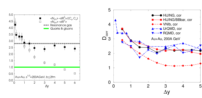
Figure 2: Left: Charge fluctuations for different rapidity windows as obtained in the URQMD model. Open symbols: without correction for global charge conservation. Full symbols: With correction for global charge conservation. Right: Results for different transport model including the parton cascade [63]. These results are corrected for charge conservation.

For large $\Delta y$ the results have to be corrected for charge conservation effects; if all charges are accepted, global charge conservation leads to vanishing fluctuations (open symbols in Fig.2). This can be corrected for as explained in the previous section (for details see [15]). The resulting values for $D$ are shown as full symbols in Fig.2. They agree nicely with the prediction for the resonance gas, as they should, since the URQMD model does not contain any partonic degrees of freedom. For small $\Delta y$ the correlations imposed by the resonances are lost, because only one of the decay products is accepted. As a result we see an increase of $D$. The right figure shows a comparison of several transport models, including the Parton Cascade model [29]. This model starts with partons in the initial state, but has some model for hadronization included. If the general ideas about the reduced charge fluctuations are correct, this model should lead to smaller values of $D$, and it does.

For very small $\Delta y$, when $\left\langle N\right\rangle\simeq 1$, the ratio $D$ is not well defined for events with $N_{-}=0$, and, therefore, cannot serve as a observable. Alternative observables, measuring the same quantity have been proposed and studied in [49].

4 Kaon Fluctuations

As discussed in section 2 at low energy the strangeness conservation has to be treated explicitly. This can be utilized to determine the degree of equilibration reached in these collisions [36]. By measuring the ratio

$$F_{2}=\frac{\left\langle N_{K}(N_{K}-1)\right\rangle}{\left\langle N_{K}\right\rangle^{2}}$$ (174)

of the number of kaon pairs over the square of the inclusive number of kaons a factor two sensitivity on the degree of equilibrium can be obtained. From transport models (see e.g. [17]) it is known, that most of the kaons are produced in secondary collisions, i.e. during the evolution of the fireball. Transport calculations also find that the equilibration time of kaons is of the order of $500\rm fm/c$, which is about ten time the lifetime of the system. Hence these models would not predict equilibration of the kaons. However, observed particle ratios including kaons are also consistent with a thermal model description (for a review see [18]). The measurement of $F_{2}$ can resolve this issue and point to new physics such as multi-particle processes, in medium effects etc., if indeed it is found to be consistent with equilibrium. This is demonstrated in Fig.3 where the time evolution of $F_{2}$ for several initial kaon numbers is shown. In all cases, $F_{2}$ quickly rises close to $F_{2}\simeq 1$ before it settles at the final equilibrium value of $F_{2}^{\rm eq.}\simeq 1/2$.

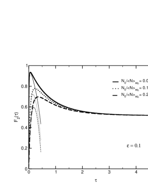
Figure 3: Time evolution of $F_{2}$ for various initial kaon numbers. The thin lines are analytical results for early times.

Thus, by measuring $F_{2}$ one can directly determine how close to chemical equilibrium the system has developed, before it freezes out. If the predictions of the transport models are correct, then a value of $F_{2}\simeq 1$ should be found. If, on the other hand, equilibrium is indeed reached in these collisions, then $F_{2}\simeq\frac{1}{2}$. In principle a similar measurement can also be done at higher energies for charmed mesons. To which extent this is technically feasible is another question.

Let us conclude the section by mentioning other observables. In the context of so called DCC production [50], the fluctuations of the fraction of neutral pions is considered a useful signal. Also the fluctuations of the elliptic flow has be proposed as an useful observable [47], which may reveal new configurations such as sphalerons, which could be created in heavy ion collisions.

6 Experimental Situation

1 Fluctuation in elementary collisions

By now, it is clear that Quantum Chromodynamics is the right theory of strong interaction. However, essential non-perturbative nature of the strong interaction still remains a difficulty. In heavy ion collisions, this is more manifest in the sense that even the hard part of the spectrum is strongly influenced by the surrounding soft medium through multiple scatterings. Therefore, before we begin to consider the experimental results from heavy ion collisions, it is crucial that we understand elementary collision results such as proton-proton collision results since these elementary collision results can provide unbiased baseline.

A large amount of data for $pp$ collisions at various beam energies were taken from Fermi Lab in the 1970’s [19, 39, 38, 40] (see also Ref.[61]). Among them, data at the beam energy of $205\,\hbox{\,GeV}$ were most thoroughly analyzed by Kafka et.al.[38, 39]. First, let us consider the ‘charge fluctuation study’. In the case of $pp$ collisions, the definition of ‘charge fluctuation’, however, differs from ours. Let us define the charge transfer

$$u(y)={1\over 2}\left[Q_{f}(y)-Q_{b}(y)\right]$$ (175)

where $Q_{f}(y)$ is the sum of the charges of the particles with rapidity larger than $y$ and $Q_{b}(y)$ is the sum of the charges of the particles with rapidity smaller than than $y$. We then define the charge transfer fluctuation

$$\left\langle\delta u(y)^{2}\right\rangle_{\rm ebe}=\left\langle u^{2}(y)\right\rangle_{\rm ebe}-\left\langle u(y)\right\rangle_{\rm ebe}^{2}$$ (176)

This quantity is usually referred to as ‘charge fluctuation’ in literature dealing with proton-proton collisions. This charge transfer fluctuation is certainly not the same as what we have been discussing so far which is the charge fluctuation within a given phase space window $\Delta\eta$. However, as we will show shortly, $\left\langle\delta u(y)^{2}\right\rangle$ is intimately related to the charge correlation functions. By considering the charge transfer fluctuation, we can then put a constraint on possible forms of the correlation functions.

To do so, consider again our simple model defined by Eq.(81). As before, we impose the conditions $M_{+}-M_{-}=Q_{c}=0$, $f_{+}=f_{-}=f$ and $h_{+}=h_{-}=h$. After straightforward but tedious algebra, we obtain

$$\left\langle\delta u(y)^{2}\right\rangle_{\rm ebe} = \left(\left\langle M_{+}\right\rangle+\left\langle M_{-}\right\rangle\right)\int_{y}^{\infty}dy^{\prime}\,f(y^{\prime})\int^{y}_{-\infty}dy^{\prime\prime}\,f(y^{\prime\prime})$$ (177)

$${}+2\left\langle M_{0}\right\rangle\int_{y}^{\infty}dy_{+}\int_{-\infty}^{y}dy_{-}f_{0}(y_{+},y_{-})$$

using the rapidity $y$ as the phase space variable.

In Ref.[38], it is shown that the data satisfies

$$\left\langle\delta u(y)^{2}\right\rangle_{\rm ebe}\approx 0.62{dN_{\rm ch}\over dy}$$ (178)

at the beam energy of $205\,\hbox{\,GeV}$ and the shape of $dN_{\rm ch}/dy$ is very well represented by a Gaussian with $\sigma^{2}_{y}\approx\log(\sqrt{s}/2m_{N})\approx 2.2$. This result puts a condition on possible forms of $f$ and $f_{0}$. In our model, the rapidity distribution of the charged particle is

$${dN_{\rm ch}\over dy}=\left(\left\langle M_{+}\right\rangle+\left\langle M_{-}\right\rangle\right)f(y)+2\left\langle M_{0}\right\rangle h(y)$$ (179)

First, let us see if charge particles alone can satisfy Eq.(178). For this to be possible we must have $\int_{y}^{\infty}dy^{\prime}\,f(y^{\prime})\int^{y}_{-\infty}dy^{\prime\prime}\,f(y^{\prime\prime})\propto f(y)$ and $\int f=1$. These conditions are satisfied by

$$f(y)={1\over 2\tilde{y}}\,{\rm sech}^{2}(y/\tilde{y})$$ (180)

where $\tilde{y}$ is a constant specifying the width of the distribution. This form of $f(y)$ is however, too sharply peaked to be consistent with the data. On the other hand a Gaussian with the above $\sigma_{y}^{2}$ can approximately satisfy the condition $\int_{y}^{\infty}dy^{\prime}\,f(y^{\prime})\int^{y}_{-\infty}dy^{\prime\prime}\,f(y^{\prime\prime})\propto f(y)$. But in this case, the proportionality constant at $y=0$ is close to 1. All this indicates that we need the correlation term involving $f_{0}(y_{+},y_{-})$.

The condition (178) can be approximately satisfied if $f_{0}$ has the following form

$$f_{0}(y_{1},y_{2})=q(y_{1}-y_{2})g((y_{1}+y_{2})/2)$$ (182)

where $q(y)$ is a sharply peaked function at $y=0$ with a small width $\Delta$, and $g(y)\approx({1/\left\langle N\right\rangle})dN/dy$. Then it can be also shown that $h(y)\approx g(y)$ and

$$\int_{y}^{\infty}dy^{\prime}\int^{y}_{-\infty}dy^{\prime\prime}f_{0}(y^{\prime},y^{\prime\prime})\approx C\,\Delta\,h(y)$$ (183)

with some constant $C<1$. In fact the authors of Ref.[38] argued that their proton-proton result is consistent with having only the neutral clusters. In our language, that corresponds to $\left\langle M_{\pm}\right\rangle=0$.

What the above consideration implies for our charge fluctuation is somewhat unclear. To the authors’ knowledge, direct measurement of charge fluctuation in the sense defined in the previous sections has not been carried out in proton-proton experiments. What have been measured are the $C_{\alpha\beta}$ functions defined in Eq.(69). In Ref[39], the maximum height at $y_{1}=y_{2}=0$ are given as

$$C_{++}(0,0)\approx 0.36$$

$$C_{--}(0,0)\approx 0.25$$

$$C_{+-}(0,0)\approx 0.5$$ (184)

Using also the overall shape given in the same reference and the fact[38] that $\left\langle N_{\rm ch}\right\rangle\approx 6$ at this energy one can then infer that

$${\left\langle\delta Q^{2}\right\rangle_{\Delta\eta}\over\left\langle N_{\rm ch}\right\rangle_{\Delta\eta}}\approx 0.5\sim 0.6$$ (185)

within $-1<y<1$ without any charge conservation corrections. Correcting for charge conservation is a difficult task to perform. If as asserted in Ref.[38] all particles are produced via neutral clusters, then there is no correction to perform. If however, some charged particles are emitted independently, then this is the lower bound. A more thorough analysis of the available data can undoubtedly yield more accurate estimate of the charge fluctuation. However, that is clearly beyond the scope of this review. We just make a remark here that our estimate of the charge fluctuation in QGP scenario ${\left\langle\delta Q^{2}\right\rangle_{\Delta\eta}/\left\langle N_{\rm ch}\right\rangle_{\Delta\eta}}\approx 0.25\sim 0.3$, seems to be still substantially smaller than the above proton-proton collision result.

2 Fluctuations in Heavy Ion Reactions

Unfortunately at the time of the writing of this review, very few published data on fluctuations in heavy ion collisions are available. Quite a few preliminary results are being discussed at conferences, which we will briefly mention. But we feel that an in depth discussion of these results prior to publication is not appropriate. The pioneering event-by-event studies have been carried out by the NA49 collaboration. They have analyzed the fluctuations of the mean transverse momentum [5] and the kaon to pion ratio [4]. Both measurements have been carried out at at the CERN SPS at slightly forward rapidities. In Fig. 4 the resulting distributions are shown together with that from mixed events (histograms). In both cases the mixed event can essentially account for the observed signal, leaving little room for genuine dynamical fluctuations. Specifically, NA49 gives $\Phi_{p_{t}}=0.6\pm 1.0\,\rm MeV$ for the transverse momentum fluctuations, which is compatible with zero. For the kaon to pion ratio they extract a width due to non-statistical fluctuations of $\sigma_{non_{s}tat}=2.8\%\pm 0.5\%$, which would be compatible form the expectations of resonance decays [34].

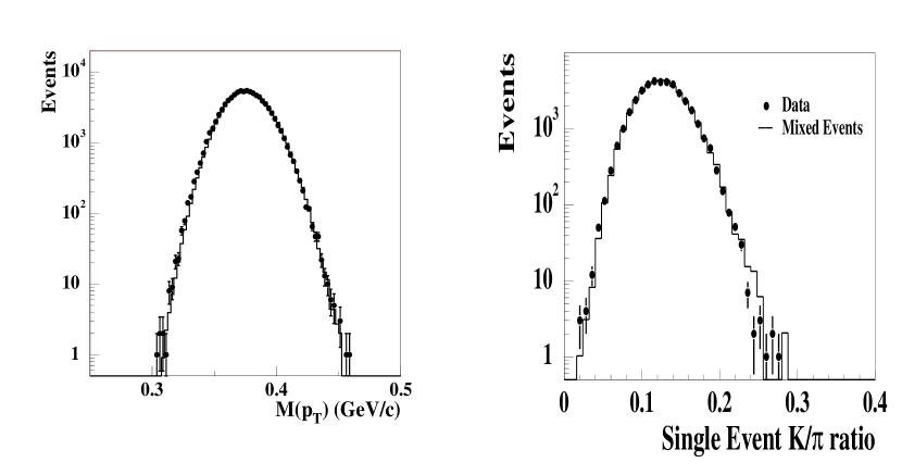
Figure 4: Results for the fluctuations of the mean transverse momentum (left) and kaon to pion ratio (right). Both results are from the NA49 collaboration.

The PHENIX collaboration recently also reported their results on mean transverse momentum and energy fluctuations at RHIC energies [2]. Similar to NA49, their result is compatible with the statistical fluctuations only, leaving no room for significant dynamical fluctuations. Their measurement was around mid-rapidity with a small azimuthal acceptance of $\Delta\Phi=58^{\circ}$

In contrast to that preliminary results by both the CERES collaboration [21] at the CERN SPS, as well as the STAR collaboration [51] at RHIC report significant dynamical fluctuations of the mean transverse momentum. Both measure at mid-rapidity. It remains to be seen if these difference in measurements can be attributed simply to the different acceptance regions covered.

As far as the charge fluctuations are concerned, first results have been reported. PHENIX [3] at RHIC which measures with a small rapidity acceptance, finds charge fluctuations consistent with a resonance gas. CERES [21] and NA49 [16], which both measure at SPS energies, report preliminary results on charge fluctuations, which are consistent with a pure pion gas. However, at the SPS the overall rapidity distribution is rather narrow, so that the correlation effect of the resonance gets lost when correcting for charge conservation [62]. But certainly, non of the measurements is even close to the prediction for the QGP. These findings have prompted ideas, that possibly a constituent quark plasma, without gluons, has been produced [11]. However, the measurement of additional observables would be needed in order to distinguish this from a hadronic gas.

But maybe the present range of $\Delta y$ is so small, that the charge fluctuations have time to assume the value of the resonance gas. As shown in Fig. 2, the results for the parton cascade arrive at the predicted value for the QGP only for $\Delta y\geq 3$. None of the present experiments has such a coverage yet and thus a detailed analysis of $D$ as a function of $\Delta y$ is needed, before any firm conclusions can be drawn.

The Balance function measurement at $\sqrt{s}=130\,\hbox{\,GeV}$ has been reported by STAR collaboration[24]. Going from peripheral to central collisions, the width of balance function steadily decreases. The trend is what one would expect if more of the system is filled with a QGP as the collision becomes more central. However, since the reduction is only about 20 % going from most perpheral to most central, it is not yet clear whether this signals the presence of a QGP or more mundane effect such as the strong flow.

7 Conclusions and Outlook

In this review we discussed several aspects of the emerging field of event-by-event fluctuations in heavy ion collisions. We have briefly reviewed the basics concepts of fluctuations in a thermal system, and we have discussed the possible connection between a idealized thermal system and a “real world” heavy ion collision. Furthermore we have introduced the variables used in order to present fluctuations and discussed the relation between them. Finally we have present the presently published data, which are rather limited. But this is soon going to change.

Crucial for the understanding of fluctuations is the connections to correlation functions. While the concept of fluctuations might be more intuitive and thus might lead us to new insights and approaches, the relevant information is encoded in the correlation functions. For example, consider the charge fluctuations, which we have discussed in some detail. It is true that like-sign and unlike-sign correlation functions encode all the necessary information on the charge fluctuations. However the physical meanings of those encoded information can be made clear only through considering charge fluctuations in and out of QGP and its connection to the relevant features of the correlation functions. But certainly from the observational point of view, the information to be extracted are the correlation functions between all possible quanta. Once they are available, the relevant observables can be readily obtained by folding the correlation functions with the appropriate variables

On important aspect relevant to heavy ion collisions is the finiteness of the system. Thus approximations which are valid for a large system, such as the grand-canonical ensemble. Appropriate corrections have to be applied to either theory or data in order to extract the properties of the bulk matter. While this is not new to heavy ion physics, for the case of fluctuations these methods still require more refinement.

Since the study of fluctuations is a new and developing area of heavy ion physics, this review can only be some kind of snapshot at a “hopefully” fast developing field. By no means can it be comprehensive. Most of the experimental data are available, if at all, only in preliminary form. Furthermore analysis methods and possible new observable based on fluctuations are being developed as we write the review. Therefore our idea was to present the basic concepts as well as some of the necessary formalism in a consistent and understandable way. To which extent we have succeeded is beyond our judgment.

Acknowledgments

The authors thank S. Voloshin, L. Ray, C. Gale, C. Pruneau and S. Gavin for suggestions and discussions. V.K. was supported by the Director, Office of Science, Office of High Energy and Nuclear Physics, Division of Nuclear Physics, and by the Office of Basic Energy Sciences, Division of Nuclear Sciences, of the U.S. Department of Energy under Contract No. DE-AC03-76SF00098. S.J. thanks RIKEN BNL Center and U.S. Department of Energy [DE-AC02-98CH10886] for providing facilities essential for the completion of this work. S.J. is also supported in part by the Natural Sciences and Engineering Research Council of Canada.

References

- [1] ”e.g. COBE web page at” ”http://space.gsfc.nasa.gov/astro/cobe/cobe_home.html”.
- [2] K. Adcox et al. Event-by-event fluctuations in mean p(t) and mean e(t) in s(nn)**(1/2) = 130-gev au + au collisions. Phys. Rev., C66:024901, 2002.
- [3] K. Adcox et al. Net charge fluctuations in au + au interactions at s(nn)**(1/2) = 130-gev. Phys. Rev. Lett., 89:082301, 2002.
- [4] S. V. Afanasev et al. Event-by-event fluctuations of the kaon to pion ratio in central pb + pb collisions at 158-gev per nucleon. Phys. Rev. Lett., 86:1965–1969, 2001.
- [5] H. Appelshauser et al. Event-by-event fluctuations of average transverse momentum in central pb + pb collisions at 158-gev per nucleon. Phys. Lett., B459:679–686, 1999.
- [6] Masayuki Asakawa, Ulrich W. Heinz, and Berndt Muller. Fluctuation probes of quark deconfinement. Phys. Rev. Lett., 85:2072–2075, 2000.
- [7] Gordon Baym, B. Blattel, L. L. Frankfurt, H. Heiselberg, and M. Strikman. Correlations and fluctuations in high-energy nuclear collisions. Phys. Rev., C52:1604–1617, 1995.
- [8] Gordon Baym and Henning Heiselberg. Event-by-event fluctuations in ultrarelativistic heavy-ion collisions. Phys. Lett., B469:7–11, 1999.
- [9] Boris Berdnikov and Krishna Rajagopal. Slowing out of equilibrium near the qcd critical point. Phys. Rev., D61:105017, 2000.
- [10] George F. Bertsch. Meson phase space density from interferometry. Phys. Rev. Lett., 72:2349–2350, 1994.
- [11] A. Bialas. Charge fluctuations in a quark antiquark system. Phys. Lett., B532:249–251, 2002.
- [12] A. Bialas and V. Koch. Event by event fluctuations and inclusive distributions. Phys. Lett., B456:1–4, 1999.
- [13] J. P. Blaizot, E. Iancu, and A. Rebhan. Comparing different hard-thermal-loop approaches to quark number susceptibilities. 2002.
- [14] J. P. Blaizot, Edmond Iancu, and A. Rebhan. Quark number susceptibilities from htl-resummed thermodynamics. Phys. Lett., B523:143–150, 2001.
- [15] M. Bleicher, S. Jeon, and V. Koch. Event-by-event fluctuations of the charged particle ratio from non-equilibrium transport theory. Phys. Rev., C62:061902, 2000.
- [16] C. Blume et al. Results on correlations and fluctuations from na49. 2002.
- [17] E. L. Bratkovskaya, W. Cassing, and U. Mosel. Analysis of kaon production at sis energies. Nucl. Phys., A622:593–604, 1997.
- [18] P Braun-Munzinger, K Redlich, and J Stachel. this review volume.
- [19] C. M. Bromberg et al. Pion production in p p collisions at 102-gev/c. Phys. Rev., D9:1864–1871, 1974.
- [20] J. Cleymans, K. Redlich, and E. Suhonen. Canonical description of strangeness conservation and particle production. Z. Phys., C51:137–141, 1991.
- [21] CERES collaboration. to be published, 2002. prelimnary results, private communication.
- [22] M. Doering and V. Koch. Event-by-event fluctuations in heavy ion collisions. Acta Phys. Polon., B33:1495–1504, 2002.
- [23] V. L. Eletsky, J. I. Kapusta, and R. Venugopalan. Screening mass from chiral perturbation theory, virial expansion and the lattice. Phys. Rev., D48:4398–4407, 1993.
- [24] J.Adams et.al. Narrowing of the balance function with centrality in au + au collisions s(nn)**(1/2) = 130-gev. 2003.
- [25] Z. Fodor and S. D. Katz. Lattice determination of the critical point of qcd at finite t and mu. JHEP, 03:014, 2002.
- [26] Rajiv V. Gavai and Sourendu Gupta. The continuum limit of quark number susceptibilities. Phys. Rev., D65:094515, 2002.
- [27] M. Gazdzicki and S. Mrowczynski. A method to study ’equilibration’ in nucleus-nucleus collisions. Z. Phys., C54:127–132, 1992.
- [28] Marek Gazdzicki. A method to study chemical equilibration in nucleus nucleus collisions. Eur. Phys. J., C8:131–133, 1999.
- [29] Klaus Geiger and Berndt Muller. Dynamics of parton cascades in highly relativistic nuclear collisions. Nucl. Phys., B369:600–654, 1992.
- [30] S. Gottlieb et al. Thermodynamics of lattice qcd with two light quark flavours on a 16**3 x 8 lattice. ii. Phys. Rev., D55:6852–6860, 1997.
- [31] Ulrich W. Heinz and Barbara V. Jacak. Two-particle correlations in relativistic heavy-ion collisions. Ann. Rev. Nucl. Part. Sci., 49:529–579, 1999.
- [32] H. Heiselberg and A. D. Jackson. Anomalous multiplicity fluctuations from phase transitions in heavy ion collisions. Phys. Rev., C63:064904, 2001.
- [33] Henning Heiselberg. Event-by-event physics in relativistic heavy-ion collisions. Phys. Rept., 351:161–194, 2001.
- [34] S. Jeon and V. Koch. Fluctuations of particle ratios and the abundance of hadronic resonances. Phys. Rev. Lett., 83:5435–5438, 1999.
- [35] S. Jeon and V. Koch. Charged particle ratio fluctuation as a signal for qgp. Phys. Rev. Lett., 85:2076–2079, 2000.
- [36] S. Jeon, V. Koch, K. Redlich, and X. N. Wang. Fluctuations of rare particles as a measure of chemical equilibration. Nucl. Phys., A697:546–562, 2002.
- [37] Sang-yong Jeon and Scott Pratt. Balance functions, correlations, charge fluctuations and interferometry. Phys. Rev., C65:044902, 2002.
- [38] T. Kafka et al. Charge and multiplicity fluctuations in 205-gev/c p p interactions. Phys. Rev. Lett., 34:687–690, 1975.
- [39] T. Kafka et al. One, two, and three particle distributions in p p collisions at 205-gev/c. Phys. Rev., D16:1261, 1977.
- [40] T. Kafka et al. Correlations between neutral and charged pions produced in 300-gev/c p p collisions. Phys. Rev., D19:76, 1979.
- [41] J. Kapusta. Finite Temperature Field Theory. Cambridge University Press, 1989.
- [42] C. M. Ko et al. Kinetic equation with exact charge conservation. Phys. Rev. Lett., 86:5438–5441, 2001.
- [43] V. Koch, M. Bleicher, and S. Jeon. Event-by-event fluctuations and the qgp. Nucl. Phys., A698:261–268, 2002.
- [44] L Landau and L.M. Lifshitz. Statistical Physics. Pergamon Press, New York, 1980.
- [45] Zi-wei Lin and C. M. Ko. Baryon number fluctuation and the quark gluon plasma. Phys. Rev., C64:041901, 2001.
- [46] Stanislaw Mrowczynski. Transverse momentum and energy correlations in the equilibrium system from high-energy nuclear collisions. Phys. Lett., B439:6–11, 1998.
- [47] Stanislaw Mrowczynski and Edward V. Shuryak. Elliptic flow fluctuations. 2002.
- [48] Madappa Prakash, Ralf Rapp, Jochen Wambach, and Ismail Zahed. Isospin fluctuations in qcd and relativistic heavy-ion collisions. Phys. Rev., C65:034906, 2002.
- [49] C. Pruneau, S. Gavin, and S. Voloshin. Methods for the study of particle production fluctuations. 2002.
- [50] Krishna Rajagopal. The chiral phase transition in qcd: Critical phenomena and long wavelength pion oscillations. 1995.
- [51] R. L. Ray. Correlations, fluctuations, and flow measurements from the star experiment. 2002. Proceedings Quark Matter 2002, Nantes, France, July 2002.
- [52] F. Reif. Fundamentals of Statistical and Thermal Physics. McGraw-Hill, 1984.
- [53] Edward V. Shuryak. Event-per-event analysis of heavy ion collisions and thermodynamical fluctuations. Phys. Lett., B423:9–14, 1998.
- [54] Edward V. Shuryak and Misha A. Stephanov. When can long range charge fluctuations serve as a qgp signal? Phys. Rev., C63:064903, 2001.
- [55] Misha A. Stephanov, K. Rajagopal, and Edward V. Shuryak. Signatures of the tricritical point in QCD. Phys. Rev. Lett., 81:4816–4819, 1998.
- [56] Misha A. Stephanov, K. Rajagopal, and Edward V. Shuryak. Event-by-event fluctuations in heavy ion collisions and the QCD critical point. Phys. Rev., D60:114028, 1999.
- [57] L. Stodolsky. Temperature fluctuations in multiparticle production. Phys. Rev. Lett., 75:1044–1045, 1995.
- [58] C. Sturm et al. Kaon and antikaon production in dense nuclear matter. J. Phys., G28:1895–1902, 2002.
- [59] M. J. Tannenbaum. The distribution function of the event-by-event average p(t) for statistically independent emission. Phys. Lett., B498:29–34, 2001.
- [60] S Voloshin, V Koch, and H.G. Ritter. Event-by-event fluctuations in collective quantities. Phys. Rev., C60:0224901, 1999.
- [61] J. Whitmore. Multiparticle production in the fermilab bubble chambers. Phys. Rept., 27:187–273, 1976.
- [62] Jacek Zaranek. Measures of charge fluctuations in nuclear collisions. Phys. Rev., C66:024905, 2002.
- [63] Q. H. Zhang, V. Topor Pop, S. Jeon, and C. Gale. Charged particle ratio fluctuations and microscopic models of nuclear collisions. Phys. Rev., C66:014909, 2002.