1 Introduction

If supersymmetry (SUSY) as the most attractive extension of the Standard Model is realized at low energies, the next generation of high energy physics experiments at Tevatron, LHC and a future $e^{+}e^{-}$ linear collider will discover supersymmetric particles. Particularly at a linear collider, it will be possible to perform measurements with high precision [1, 2] which allows to test the underlying SUSY model. For instance, at TESLA [1] the precision of the mass determination of charginos and neutralinos, the supersymmetric partners of the gauge and Higgs bosons, will be $\Delta m_{\tilde{\chi}^{\pm,0}}=0.1-1$ GeV. To match this accuracy it is indispensable to include higher order radiative corrections.
One goal of all analyses based on precise measurements of cross sections, decay branching ratios, masses of supersymmetric particles, etc. will be the reconstruction of the fundamental parameters of the underlying supersymmetric model. In particular, this is needed for extrapolating the parameters to the GUT point to check the unification of the supersymmetry breaking parameters [3, 4].
In the Minimal Supersymmetric Standard Model (MSSM) the chargino and neutralino system depends on the parameters $M$, $M^{\prime}$, $\mu$ and $\tan\beta$. $M$ and $M^{\prime}$ are the SU(2) and U(1) gauge mass parameter, $\mu$ is the higgsino mass parameter and $\tan\beta=\frac{v_{2}}{v_{1}}$ with $v_{1,2}$ the vacuum expectation values of the two neutral Higgs doublet fields. At lowest order, it was shown in [5, 6] that these parameters can be extracted from the masses and production cross sections in $e^{+}e^{-}$ collisions with polarized electron beams. At higher order, this extraction of the parameters is, however, not trivial. It depends on the definition of the mass matrices (at higher order) and on the renormalization scheme. This is the subject of this paper.
In the (scale dependent) $\overline{\rm DR}$ scheme the one–loop corrections to the chargino/neutralino mass matrix were calculated in [7, 8]. In [9] effective chargino mixing matrices were introduced, which are independent of the renormalization scale. For the on–shell renormalization of the chargino and neutralino system which we adopt here, two methods were proposed [10, 11]. They differ by different counter terms to the parameters $M^{\prime}$, $M$ and $\mu$. Although both schemes are equivalent in the sense that the observables (masses, cross sections, branching ratios, etc.) are the same, the meaning of the parameters $M$, $M^{\prime}$, $\mu$ extracted are different. In the following we want to analyze in detail the determination of the parameters of the chargino/neutralino mass matrices at one–loop level in the scheme [11]. We will point out that at one–loop level the values of the on–shell parameters $M$ and $\mu$ depend on whether they are determined from the chargino or neutralino system. Another interesting issue is how the GUT relation $M^{\prime}=c\,M$ ($c=\frac{5}{3}\tan^{2}\theta_{W}$ in SU(5), $c=11\tan^{2}\theta_{W}$ in AMSB) valid in the $\overline{\rm DR}$ scheme can be tested if the on–shell values of $M^{\prime}$ and $M$ are extracted from experiment. The one–loop corrections will also change the gaugino and higgsino nature of the charginos and neutralinos, in particular also of the lightest neutralino. This is important for the dark matter search [12, 13, 14]. The whole analysis is based on a full one–loop calculation within the MSSM. The corresponding formulae are given in the Appendix.

2 The chargino–neutralino sector

In the CP conserving MSSM the chargino mass matrix has at tree–level the form

$$\tilde{X}=\left(\begin{array}[]{cc}M&\sqrt{2}\,m_{W}\sin\beta\\ \sqrt{2}\,m_{W}\cos\beta&\mu\end{array}\right)\,,$$ (1)

where we take $M$, $\mu$, $m_{W}$ and $\tan\beta$ as on–shell parameters. $M$ and $\mu$ are taken real. With the real rotation matrices $U$ and $V$

$$U=\left(\begin{array}[]{cc}\cos\Phi_{L}&\sin\Phi_{L}\\ -\sin\Phi_{L}&\cos\Phi_{L}\end{array}\right)\,,\quad V=\left(\begin{array}[]{cc}\cos\Phi_{R}&\sin\Phi_{R}\\ -\sin\Phi_{R}&\cos\Phi_{R}\end{array}\right)$$ (2)

it can be diagonalized,

$$U\,\tilde{X}\,V^{T}=\mbox{diag}(\varepsilon_{1}\,\tilde{m}_{{\tilde{\chi}^{+}}_{1}},\ \varepsilon_{2}\,\tilde{m}_{{\tilde{\chi}^{+}}_{2}})\,,$$ (3)

with $\varepsilon_{i}=\pm 1$ and the tree–level masses $\tilde{m}_{{\tilde{\chi}^{+}}_{1}}<\tilde{m}_{{\tilde{\chi}^{+}}_{2}}$. The solutions of eq. (3) are

$$\tan 2\Phi_{L}=\frac{2\sqrt{2}m_{W}(M\cos\beta+\mu\,\sin\beta)}{M^{2}-\mu^{2}-2m_{W}^{2}\cos 2\beta}\,,\quad\tan 2\Phi_{R}=\frac{2\sqrt{2}m_{W}(\mu\,\cos\beta+M\sin\beta)}{M^{2}-\mu^{2}+2m_{W}^{2}\cos 2\beta}\,,$$ (4)

and

$$\tilde{m}_{{\tilde{\chi}^{+}}_{1,2}}^{2}=\frac{1}{2}\left(M^{2}+\mu^{2}+2m_{W}^{2}\mp\sqrt{(M^{2}+\mu^{2}+2m_{W}^{2})^{2}-4(M\mu-m_{W}^{2}\sin 2\beta)^{2}}\right)\,.$$ (5)

As shown in [11], the on–shell mass matrix $X$ at one–loop level can be written as a sum of the tree–level mass matrix $\tilde{X}$ in terms of the on–shell parameters as in (1) and the ultraviolet finite shifts $\Delta X$

$$X=\tilde{X}+\Delta X\,.$$ (6)

This implies corrections in the mass eigenvalues, $\Delta m_{{\tilde{\chi}^{+}}_{i}}$, and in the rotation angles of the coupling matrices, $\Delta\Phi_{L}$ and $\Delta\Phi_{R}$.
In the neutralino sector, we have the symmetric tree–level mass matrix

$$\tilde{Y}=\left(\begin{array}[]{cccc}M^{\prime}&0&-m_{Z}\sin\theta_{W}\cos\beta&m_{Z}\sin\theta_{W}\sin\beta\\ 0&M&m_{Z}\cos\theta_{W}\cos\beta&-m_{Z}\cos\theta_{W}\sin\beta\\ -m_{Z}\sin\theta_{W}\cos\beta&m_{Z}\cos\theta_{W}\cos\beta&0&-\mu\\ m_{Z}\sin\theta_{W}\sin\beta&-m_{Z}\cos\theta_{W}\sin\beta&-\mu&0\end{array}\right)\,.$$ (7)

Using the real matrix $Z$, we can rotate from the gauge eigenstate basis of the neutral gauginos and higgsinos $\psi_{j}^{0}=(-i\lambda^{\prime},-i\lambda^{3},\psi_{H_{1}}^{1},\psi_{H_{2}}^{2})$ to the mass eigenstate basis of the neutralinos ${\tilde{\chi}^{0}}_{i}=Z_{ij}\psi_{j}$,

$$Z\,\tilde{Y}\,Z^{T}=\mbox{diag}(\varepsilon_{1}\,\tilde{m}_{\tilde{\chi}_{1}^{0}},\,\varepsilon_{2}\,\tilde{m}_{\tilde{\chi}_{2}^{0}},\,\varepsilon_{3}\,\tilde{m}_{\tilde{\chi}_{3}^{0}},\,\varepsilon_{4}\,\tilde{m}_{\tilde{\chi}_{4}^{0}})\,.$$ (8)

Taking the one–loop terms into account

$$Y=\tilde{Y}+\Delta Y\,,$$ (9)

we again obtain corrections in the masses, $\Delta m_{{\tilde{\chi}^{0}}_{i}}$, and in the coupling matrix $Z=\tilde{Z}+\Delta Z$.

3 Parameter fixing

In supersymmetry one has several mass matrices due to the mixing of interaction states. We define the on–shell mass matrix such that all elements which are non–zero at tree–level have formally the tree–level form but give the physical masses and rotation matrices. We always start with a certain set of on-shell input parameters. For these we need fixing conditions. All other on-shell entries in the mass matrices can then be calculated.
The Standard Model input parameters are the pole masses $m_{W}=80.423$ GeV and $m_{Z}=91.1876$ GeV. The Weinberg angle $\theta_{W}$ is fixed by $\cos\theta_{W}=m_{W}/m_{Z}$ [15]. The SUSY parameter $\tan\beta$ is fixed by the condition that there is no transition from the physical CP odd Higgs particle $A^{0}$ to the vector boson $Z^{0}$ [16], $\textrm{Im}\,\hat{\Pi}_{A^{0}Z^{0}}(m_{A}^{2})\,=0$ which gives the counter term $\delta\tan{\beta}={\textrm{Im}\,}{\Pi}_{A^{0}Z^{0}}(m_{A}^{2})/(2m_{Z}\cos^{2}\beta)$. $\hat{\Pi}_{A^{0}Z^{0}}$ is the renormalized self–energy for the mixing of $A^{0}$ and $Z^{0}$. In this study, the physical input for calculating our input on-shell parameters $M$, $\mu$, and $M^{\prime}$ are the two chargino masses and one neutralino mass. For the other SUSY parameters we use the simplifications $A_{t}=A_{b}=A_{\tau}=A$ for the trilinear couplings and $M_{\tilde{Q}_{1,2}}=M_{\tilde{U}_{1,2}}=M_{\tilde{D}_{1,2}}=M_{\tilde{L}_{1,2}}=M_{\tilde{E}_{1,2}}$, $M_{\tilde{Q}_{3}}=\frac{10}{9}M_{\tilde{U}_{3}}=\frac{10}{11}M_{\tilde{D}_{3}}=M_{\tilde{L}_{3}}=M_{\tilde{E}_{3}}=M_{\tilde{Q}}$ for the soft breaking sfermion mass parameters.
In the $\overline{\rm DR}$ scheme (at a scale $Q$) the parameters $\hat{M}$ and $\hat{\mu}$ are the same in the chargino and neutralino sector. However, the on–shell parameters $M$ and $\mu$ get different one–loop corrections and thus have different on–shell values due to different thresholds:

$$\hat{M}(Q)=M+\delta M(Q)=M^{{\tilde{\chi}^{+}}}+\delta X_{11}=M^{{\tilde{\chi}^{0}}}+\delta Y_{22}\,,$$ (10)

$$\hat{\mu}(Q)=\mu+\delta\mu(Q)=\mu^{{\tilde{\chi}^{+}}}+\delta X_{22}=\mu^{{\tilde{\chi}^{0}}}-\delta Y_{34}\,.$$ (11)

$\delta X_{ij}$, $\delta Y_{ij}$ are the counter terms to the elements $X_{ij}$, $Y_{ij}$ of the chargino and neutralino mass matrix. The corresponding expressions are given in the Appendix. The finite difference can be expressed in terms of the chargino and neutralino mass matrix counter terms

$$\Delta M \equiv M^{\tilde{\chi}^{+}}-M^{\tilde{\chi}^{0}}=\ \ \ \ \delta Y_{22}-\delta X_{11}\,,$$ (12)

$$\Delta\mu\ \equiv \mu^{\tilde{\chi}^{+}}\ -\ \mu^{\tilde{\chi}^{0}}\ =-(\delta Y_{34}+\delta X_{22})\,.$$ (13)

Therefore, we have the freedom to define the input on–shell parameters $M$ and $\mu$ in the chargino sector, i.e. $M\equiv M^{\tilde{\chi}^{+}}=X_{11}$, $\mu\equiv\mu^{\tilde{\chi}^{+}}=X_{22}$, and obtain corrections in the neutralino sector, or fix $M$ and $\mu$ in the neutralino sector, i.e. $M\equiv M^{\tilde{\chi}^{0}}=Y_{22}$, $\mu\equiv\mu^{\tilde{\chi}^{0}}=-Y_{34}$, and get corrections in the chargino mass matrix. For a particular physical situation the elements of the one–loop mass matrices $X$ and $Y$ (with on–shell parameters plus corrections) are given by the measured neutralino, chargino masses and other observables, e.g. cross sections.
If $M$ and $M^{\prime}$ are independent parameters it is convenient to use for the on-shell $M^{\prime}$ the definition $Y_{11}\equiv M^{\prime}=\tilde{Y}_{11}$. If the SU(5) GUT relation, $\hat{M}^{\prime}=\frac{5}{3}\tan^{2}\hat{\theta}_{W}\,\hat{M}$, holds for the $\overline{\rm DR}$ parameters $\hat{M}$ and $\hat{M}^{\prime}$, we obtain a finite shift for the on–shell parameters. Thus we can write $Y_{11}\equiv M^{\prime}=\frac{5}{3}\tan^{2}\theta_{W}\,M+\Delta Y_{11}$, with

$$\Delta Y_{11}\;=\;\bigg{(}\frac{2}{\cos^{2}{\theta_{W}}}\,\frac{\delta\sin\theta_{W}}{\sin\theta_{W}}\,+\,\frac{\delta M}{M}\bigg{)}\,Y_{11}\;-\;\delta Y_{11}\,.$$ (14)

The correction $\Delta Y_{11}$ is due to the same effect and of the same order as $\Delta M$ and $\Delta\mu$, eq.(12) and (13). Therefore we include it in our calculations in the cases where gauge unification is explicitly assumed. Because $M$ depends on the fixing this is also the case for $\Delta Y_{11}$. Let $\Delta Y_{11}^{{\tilde{\chi}^{+}}}$ be the correction in the case, where $M$ is fixed in the chargino sector, and $\Delta Y_{11}^{{\tilde{\chi}^{0}}}$ the case, where $M$ is fixed in the neutralino sector, it follows

$$\Delta Y_{11}^{{\tilde{\chi}^{+}}}-\Delta Y_{11}^{{\tilde{\chi}^{0}}}=\frac{5}{3}\tan^{2}\theta_{W}\,\Delta M\,.$$ (15)

In Fig. 1 the mass corrections for the lightest neutralino and chargino assuming gauge unification are shown as a function of $M$. If $M$ and $\mu$ are fixed in the neutralino sector (dashed lines) we have $Y_{22}\equiv M^{{\tilde{\chi}^{0}}}=M$, $X_{11}\equiv M^{{\tilde{\chi}^{+}}}=M+\Delta M$, $Y_{34}\equiv-\mu^{\tilde{\chi}^{0}}=-\mu$, $X_{22}\equiv\mu^{\tilde{\chi}^{+}}=\mu+\Delta\mu$ and $Y_{11}=\frac{5}{3}\tan^{2}\theta_{W}M+\Delta Y_{11}^{\tilde{\chi}^{0}}$. If $M$ and $\mu$ are fixed in the chargino sector (full lines) we get $Y_{22}\equiv M^{{\tilde{\chi}^{0}}}=M-\Delta M$, $X_{11}\equiv M^{{\tilde{\chi}^{+}}}=M$, $Y_{34}\equiv-\mu^{\tilde{\chi}^{0}}=-(\mu-\Delta\mu)$, $X_{22}\equiv\mu^{\tilde{\chi}^{+}}=\mu$ and $Y_{11}=\frac{5}{3}\tan^{2}\theta_{W}M+\Delta Y_{11}^{\tilde{\chi}^{+}}$. The differences between the full and the dashed line are due to $\Delta M$ and $\Delta\mu$, eqs. (12), (13) and (15).

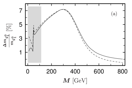
Figure 1: Relative corrections to the ${\tilde{\chi}^{0}}_{1}$ and ${\tilde{\chi}^{+}}_{1}$ masses with gauge unification, fixing $M$ and $\mu$ in the chargino (full lines) and neutralino (dashed lines) sector. The parameters are {$m_{A^{0}}$, $\tan\beta$, $M_{\tilde{Q}_{1}}$, $M_{\tilde{Q}}$, $A$, $\mu$} = {500, 40, 300, 300, -400, -220} GeV. The grey areas are excluded by the bound $m_{{\tilde{\chi}^{+}}_{1}}\geq 100$ GeV.

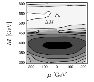
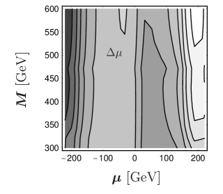
Figure 2: The corrections $\Delta M$ and $\Delta\mu$ as a function of $M$ and $\mu$ (fixed in the chargino sector) with the parameters {$m_{A^{0}}$, $\tan\beta$, $M_{\tilde{Q}_{1}}$, $M_{\tilde{Q}}$, $A$} = {500, 7, 300, 300, -500} GeV. $M^{\prime}$ fulfills the GUT relation.

In Fig. 2 the corrections $\Delta M$ and $\Delta\mu$ are given as a function of $M$ and $\mu$. For $\Delta M$ the corrections are in the range of $\Delta M=-0.2$ GeV (white) and $\Delta M=+0.6$ GeV (black). The corrections $\Delta\mu$ are between $\Delta\mu=-0.4$ GeV (white) and $\Delta\mu=+0.5$ GeV (dark grey). The difference between two lines are $0.1$ GeV.

4 Coupling corrections

With the one–loop corrections to the rotation matrices $U$, $V$ and $Z$, the gaugino and higgsino characters of the individual chargino and neutralino states change. This can have large effects on decay widths of processes where these particles are involved [17]. The character of the LSP neutralino plays a key role in dark matter theories [12, 13, 14]. In Fig. 3 the correction in the gaugino (higgsino) components of the neutralino ${\tilde{\chi}^{0}}_{i}$, $G_{i}=|Z_{i1}|^{2}+|Z_{i2}|^{2}$ ($H_{i}=|Z_{i3}|^{2}+|Z_{i4}|^{2}=1-G_{i}$), is presented. In Fig. 3a we show that the correction for the lightest neutralino is in the range of 5% (full line). In the case of gauge unification (dashed line) the additional large correction to $Y_{11}$ (approx. +10.8% at $\mu=370$ GeV) leads to a change in the gaugino component up to 30%. In Fig. 3b the corrections for all four neutralinos is given for the same parameter set. In the range between $\mu=370$ GeV and $\mu=400$ GeV, ${\tilde{\chi}^{0}}_{2}$ and ${\tilde{\chi}^{0}}_{3}$ are nearly mass–degenerated at tree–level. At one–loop the mass order and – as a consequence – the numbering changes. This is just a small effect in the mass spectrum, but the interchanging of the gaugino and higgsino components is in the range of $\pm$30%.

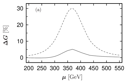
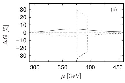
Figure 3: Corrections $\Delta G=\tilde{G}-G$ in the gaugino components as a function of $\mu$, with the parameters {$m_{A^{0}}$, $\tan\beta$, $M_{\tilde{Q}_{1}}$, $M_{\tilde{Q}}$, $A$, $M$} = {500, 20, 300, 300, -500, 700} GeV. In (a) the correction of the ${\tilde{\chi}^{0}}_{1}$ character is presented assuming the SU(5) GUT relation for the on–shell (full line) or $\overline{\rm DR}$ (dashed line) parameters $M$ and $M^{\prime}$. In (b) the corrections for all four neutralinos {${\tilde{\chi}^{0}}_{1}$, ${\tilde{\chi}^{0}}_{2}$, ${\tilde{\chi}^{0}}_{3}$, ${\tilde{\chi}^{0}}_{4}$} = {full, dashed, dotted, dash–dotted} are given (no gauge unification assumed).

5 Parameter analysis

The chargino masses $m_{{\tilde{\chi}^{+}}_{1,2}}$ and production cross sections can be measured very precisely at a future $e^{+}e^{-}$ linear collider [1, 2]. From these observables the mixing angles $\cos\Phi_{L,R}$ and by inverting the relations (4) and (5) the fundamental SUSY parameters $M$, $\mu$ and $\tan\beta$ can be obtained in lowest order [5, 6]. If a neutralino mass is known, one can also obtain $M^{\prime}$ at tree–level. However, high precision experiments will make it necessary to take into account one–loop corrections. In the following, we will compare the tree–level approximations and the full one–loop corrected fundamental SUSY parameters.
We use as input the two chargino masses, the mass of the lightest neutralino and assume the on–shell $\tan\beta$ is known from the Higgs sector [16]. Calculating the SUSY parameters $M$ and $\mu$ from the tree–level mass matrices as given in (1) and (7) leads to a four–fold ambiguity. For comparison we choose the same branch as in [10]. Because we use as input the physical masses this set of tree–level mass matrices $X^{\rm tree}$, $Y^{\rm tree}$ is different from $\tilde{X}$ and $\tilde{Y}$, which give the true tree–level mass eigenvalues. On the other hand, $X^{\rm tree}$ and $Y^{\rm tree}$ are defined to give the right physical (on–shell) chargino masses and one neutralino mass. To calculate the one–loop corrections, values for the other SUSY parameters ($A$, $M_{\tilde{Q}}$, $M_{\tilde{Q}_{1}}$, $m_{A^{0}}$) are needed. The following example, calculated for the same set of parameters as in Fig. 4 but $m_{{\tilde{\chi}^{+}}_{2}}=350$ GeV, shows the chargino and neutralino mass matrices in tree–level approximation plus the one–loop corrections,

$$Y=Y^{\rm tree}+\Delta Y^{\rm tree}=\left(\begin{array}[]{cccc}203.7&0&-2.1&42.9\\ 0&325.9&4.0&-80.3\\ -2.1&4.0&0&-147.0\\ 42.9&-80.3&-147.0&0\\ \end{array}\right)\;+\;\left(\begin{array}[]{cccc}-5.1&-0.2&-0.2&1.3\\ -0.2&1.5&-0.5&1.8\\ -0.2&-0.5&-0.1&1.0\\ 1.3&1.8&1.0&3.7\\ \end{array}\right)\,,$$

$$X=X^{\rm tree}+\Delta X^{\rm tree}=\left(\begin{array}[]{cccc}325.9&113.6\\ 5.7&147.0\\ \end{array}\right)\;+\;\left(\begin{array}[]{cccc}1.6&-3.1\\ -0.9&-1.1\\ \end{array}\right)\,.$$

Note that both $X^{\rm tree}$ ($Y^{\rm tree}$) and $X$ ($Y$) have the same physical mass eigenvalues of ${\tilde{\chi}^{+}}_{1,2}$ and ${\tilde{\chi}^{0}}_{1}$. We call the parameters used in $X^{\rm tree}$ and $Y^{\rm tree}$ effective parameters $M^{\rm eff}$, $\mu^{\rm eff}$ and $M^{\prime\rm eff}$ corresponding to the parameters used in [10]. With $Y=\tilde{Y}+\Delta Y=Y^{\rm tree}+\Delta Y^{\rm tree}$ (and the corresponding relation for the chargino mass matrix) the fundamental on–shell parameters can be determined. For instance, $M^{\prime}\equiv Y_{11}=M^{\prime\rm eff}+\Delta Y_{11}^{\rm tree}=203.7-5.1$. With $M$ fixed in the chargino system we get $M\equiv X_{11}=M^{\rm eff}+\Delta X_{11}^{\rm tree}=325.9+1.6$.
In Fig. 4 and 5a the differences between the effective parameters in $Y^{\rm tree}$, $X^{\rm tree}$ and the properly defined one–loop on–shell parameters are shown. The effective parameters are obtained applying tree–level relations on the measured masses, while the on–shell parameters are defined by the elements of the one–loop corrected mass matrices. As the effective tree–level and the one–loop corrected chargino mass matrix have the same eigenvalues, this may imply sizeable corrections in the rotation angles $\Delta\Phi_{L,R}=\Phi_{L,R}^{\rm eff}-\Phi_{L,R}$. This can be seen in Fig. 5b

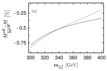
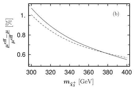
Figure 4: The relative differences between the effective and on–shell $M$ (a) and $\mu$ (b), fixing the on–shell parameters in the chargino (full line) and the neutralino (dashed line) sector with {$m_{{\tilde{\chi}^{+}}_{1}}$, $m_{{\tilde{\chi}^{0}}_{1}}$, $\tan\beta$, $m_{A^{0}}$, $M_{\tilde{Q}_{1}}$, $M_{\tilde{Q}}$, $A$} = {135, 120, 20, 600, 350, 350, 500} GeV.

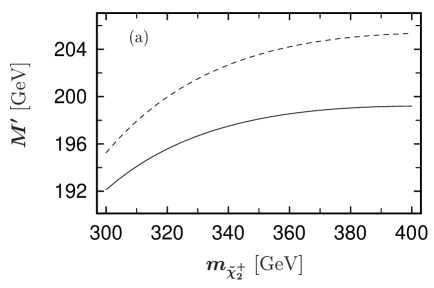
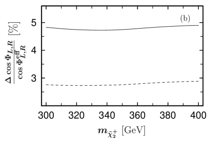
Figure 5: Fig. (a) shows the effective (dashed line) and on–shell (full line) $M^{\prime}$. In Fig. (b) there are the relative corrections to $\cos\Phi_{L}$ (full line) and $\cos\Phi_{R}$ (dashed line). The parameters are the same as in Fig. 4

If the two chargino masses are known from experiment the complete neutralino mass spectrum can be predicted by assuming the relation $\hat{M}^{\prime}=c\tan^{2}\hat{\theta}_{W}\,\hat{M}$ for the $\overline{\rm DR}$ parameters or – in the tree–level approximation – for the effective parameters. In Fig. 6 and 7 there are two different cases shown: For a SU(5) GUT ($c=\frac{5}{3}$) and an AMSB model ($c=11$). We get large corrections for the bino–like neutralino due to the correction in $Y_{11}$. This is for ${\tilde{\chi}^{0}}_{1}$ or ${\tilde{\chi}^{0}}_{3}$ (depending on $m_{{\tilde{\chi}^{+}}_{2}}$) in the SU(5) GUT scenario and ${\tilde{\chi}^{0}}_{4}$ in the AMSB model.

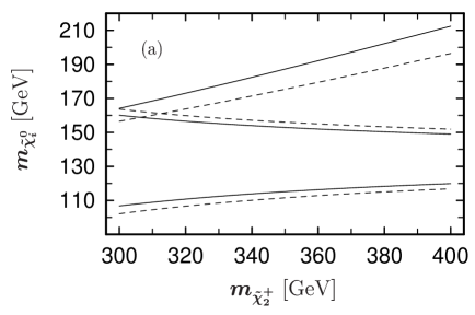
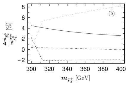
Figure 6: The neutralino mass spectrum (a) at one–loop (full) and tree–level (dashed) and the relative corrections (b) for the parameters {$m_{{\tilde{\chi}^{+}}_{1}}$, $\tan\beta$, $m_{A^{0}}$, $M_{\tilde{Q}_{1}}$, $M_{\tilde{Q}}$, $A$} = {135, 20, 600, 350, 350, 500} GeV for a SU(5) GUT model. For the mass of the ${\tilde{\chi}^{0}}_{4}$ (not shown) one has $m_{{\tilde{\chi}^{0}}_{4}}\simeq m^{\rm tree}_{{\tilde{\chi}^{0}}_{4}}\simeq m_{{\tilde{\chi}^{+}}_{2}}$. In (b) the {full, dashed, dotted, dash–dotted} line corresponds to {${\tilde{\chi}^{0}}_{1}$, ${\tilde{\chi}^{0}}_{2}$, ${\tilde{\chi}^{0}}_{3}$, ${\tilde{\chi}^{0}}_{4}$}.

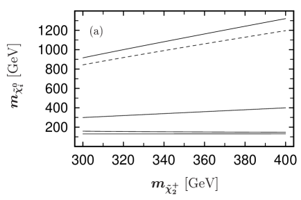
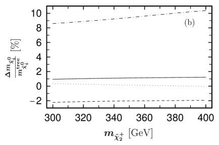
Figure 7: An AMSB model neutralino mass spectrum for the same parameters as in Fig. 6. In (a) only the tree–level approximation for the bino–like $m_{{\tilde{\chi}^{0}}_{4}}$ is shown. In (b) the {full, dashed, dotted, dash–dotted} line corresponds to {${\tilde{\chi}^{0}}_{1}$, ${\tilde{\chi}^{0}}_{2}$, ${\tilde{\chi}^{0}}_{3}$, ${\tilde{\chi}^{0}}_{4}$}.

The GUT relation can be tested by calculating the $\overline{\rm DR}$ parameters $\hat{M}(Q)=M+\delta M(Q)$, $\hat{M}^{\prime}(Q)=M^{\prime}+\delta M^{\prime}(Q)$ and $\tan\hat{\theta}_{W}(Q)=\tan\theta_{W}+\delta\tan\theta_{W}(Q)$ at a scale $Q$. Assuming such a relation for the on–shell or effective parameters is an inaccurate approximation, as shown in Fig. 8. For the given set of input parameters the ratio $\frac{\hat{M}^{\prime}}{\hat{M}\,}$ (full line) fulfills the SU(5) GUT relation at $m_{{\tilde{\chi}^{+}}_{2}}\simeq 402$ GeV. Using the effective $M^{\rm eff}$, $M^{\prime\rm eff}$ (dotted line) and the on–shell $\tan\theta_{W}$ the calculation leads to $m_{{\tilde{\chi}^{+}}_{2}}\simeq 450$ GeV. Even for the on–shell $M$ and $M^{\prime}$ the GUT point lies at $m_{{\tilde{\chi}^{+}}_{2}}\simeq 437$ GeV.

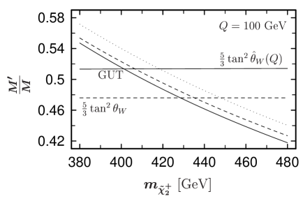
Figure 8: The ratio $\frac{M^{\prime}}{M\,}$ as a function of $m_{{\tilde{\chi}^{+}}_{2}}$. The full, dashed and dotted line corresponds to the $\overline{\rm DR}$, on–shell and effective parameters. The input parameters are the same as in Fig. 4.

6 Conclusions

We have presented a detailed discussion of the chargino and neutralino mass parameters at one–loop level. The on–shell parameters $M$, $\mu$ and $M^{\prime}$ are properly defined by the on–shell mass matrix elements. We have shown that at one–loop level the values $M$ and $\mu$ depend on whether they are determined from the chargino or neutralino system. We discussed the difference between the on–shell and the so–called effective parameters, which are obtained from observables, e.g. on–shell masses, inserted into tree–level relations. The corrections to the tree–level mass matrices in terms of the on–shell and effective parameters are discussed in different scenarios. The numerical analysis based on a complete one–loop calculation has shown that the corrections to the chargino and neutralino masses can go up to 10% and the change in the gaugino and higgsino components can be in the range of 30%. In addition, we have presented how a possible GUT relation for the parameters $M$ and $M^{\prime}$ can be tested at one–loop level.

Appendix

In the following we present the explicit formulas of all non–(s)fermionic self–energies for the neutralinos, charginos, $W$ and $Z$ bosons and the $A^{0}Z^{0}$–graphs in the MSSM. The (s)fermionic part can be found in the appendix of [11]. The two–point functions $A_{0}$, $B_{0}$, $B_{1}$ and $B_{00}$ [18] are given in the convention [19]. The neutralino and chargino mass matrix counter terms are [11]:

$$\delta X_{ij} = \frac{1}{2}\sum_{l,n=1}^{2}U_{li}V_{nj}\,{\rm Re}\left[m_{{\tilde{\chi}^{+}}_{l}}\Pi^{L}_{nl}(m_{{\tilde{\chi}^{+}}_{l}}^{2})+m_{{\tilde{\chi}^{+}}_{n}}\Pi^{R}_{ln}(m_{{\tilde{\chi}^{+}}_{n}}^{2})+\Pi^{S,R}_{nl}(m_{{\tilde{\chi}^{+}}_{l}}^{2})+\Pi^{S,L}_{ln}(m_{{\tilde{\chi}^{+}}_{n}}^{2})\right]\,,$$

$$\delta Y_{ij} = \frac{1}{2}\sum_{l,n=1}^{4}Z_{li}Z_{nj}\,{\rm Re}\left[m_{{\tilde{\chi}^{0}}_{l}}\Pi^{L}_{nl}(m_{{\tilde{\chi}^{0}}_{l}}^{2})+m_{{\tilde{\chi}^{0}}_{n}}\Pi^{R}_{ln}(m_{{\tilde{\chi}^{0}}_{n}}^{2})+\Pi^{S,R}_{nl}(m_{{\tilde{\chi}^{0}}_{l}}^{2})+\Pi^{S,L}_{ln}(m_{{\tilde{\chi}^{0}}_{n}}^{2})\right]\,,$$

with the convention

$$\Pi_{ij}(k^{2})={k/}\Big{(}P_{L}\Pi^{L}_{ij}(k^{2})+P_{R}\Pi^{R}_{ij}(k^{2})\Big{)}\,+\,P_{L}\Pi^{S,L}_{ij}(k^{2})\,+\,P_{R}\Pi^{S,R}_{ij}(k^{2})\,.$$ (A.2)

Neutralino self–energies

$$\Pi_{ij}^{H_{k}^{0}}(k)\ \ = \!\!\frac{g^{2}}{(4\pi)^{2}}\sum_{n=1}^{4}\sum_{k=1}^{2}\left[F_{nik}^{0}F_{jnk}^{0}\left(m_{\tilde{\chi}_{n}^{0}}B_{0}(k^{2},m_{\tilde{\chi}_{n}^{0}}^{2},m_{H_{k}^{0}}^{2})-{k/}B_{1}(k^{2},m_{\tilde{\chi}_{n}^{0}}^{2},m_{H_{k}^{0}}^{2})\right)\right],\hskip 22.76228pt$$ (A.3)

$$\Pi_{ij}^{A_{l}^{0}}(k)\ \ = \!\!\frac{-g^{2}}{(4\pi)^{2}}\sum_{n=1}^{4}\sum_{l=3}^{4}\left[F_{nil}^{0}F_{jnl}^{0}\left(m_{\tilde{\chi}_{n}^{0}}B_{0}(k^{2},m_{\tilde{\chi}_{n}^{0}}^{2},m_{A_{l}^{0}}^{2})+{k/}B_{1}(k^{2},m_{\tilde{\chi}_{n}^{0}}^{2},m_{A_{l}^{0}}^{2})\right)\right],$$ (A.4)

$$\Pi_{ij}^{H_{k}^{+}}(k)\hskip 2.84544pt = \sum_{n=1}^{2}\sum_{k=1}^{2}\left[\left(F_{nik}^{R}F_{njk}^{L}+F_{nik}^{L}F_{njk}^{R}\right)m_{\tilde{\chi}_{n}^{+}}B_{0}(k^{2},m_{\tilde{\chi}_{n}^{+}}^{2},m_{H_{k}^{+}}^{2})-\right.$$ (A.5)

$$\hskip 99.58464pt\left.\left(F_{nik}^{R}F_{njk}^{R}+F_{nik}^{L}F_{njk}^{L}\right){k/}B_{1}(k^{2},m_{\tilde{\chi}_{n}^{+}}^{2},m_{H_{k}^{+}}^{2})\right]\,.$$

$$\Pi_{ij}^{Z}(k)\hskip 8.5359pt = \frac{2g_{Z}^{2}}{(4\pi)^{2}}\sum_{n=1}^{4}O_{ni}^{{}^{\prime\prime}L}O_{jn}^{{}^{\prime\prime}L}\left[2m_{\tilde{\chi}_{n}^{0}}B_{0}(k^{2},m_{\tilde{\chi}_{n}^{0}}^{2},m_{Z}^{2})-{k/}B_{1}(k^{2},m_{\tilde{\chi}_{n}^{0}}^{2},m_{Z}^{2})\right]\,,$$ (A.6)

$$\Pi_{ij}^{W}(k)\hskip 5.69046pt = \frac{-2g^{2}}{(4\pi)^{2}}\sum_{n=1}^{2}\left[2\left(O_{in}^{R}O_{jn}^{L}+O_{in}^{L}O_{jn}^{R}\right)m_{\tilde{\chi}_{n}^{+}}B_{0}(k^{2},m_{\tilde{\chi}_{n}^{+}}^{2},m_{W}^{2})+\right.$$ (A.7)

$$\hskip 99.58464pt\left.\left(O_{in}^{L}O_{jn}^{L}+O_{in}^{R}O_{jn}^{R}\right){k/}B_{1}(k^{2},m_{\tilde{\chi}_{n}^{+}}^{2},m_{W}^{2})\right]\,.$$

Chargino self–energies

$$\Pi_{ij}^{H_{k}^{0}}(k) = -\frac{g^{2}}{(4\pi)^{2}}\sum_{n=1}^{2}\sum_{k=1}^{2}\left[{k/}\left(F_{nik}^{+}F_{njk}^{+}P_{R}+F_{ink}^{+}F_{jnk}^{+}P_{L}\right)B_{1}(k^{2},m_{\tilde{\chi}_{n}^{+}}^{2},m_{H_{k}^{0}}^{2})-\right.$$ (A.8)

$$\hskip 56.9055pt\left.m_{\tilde{\chi}_{n}^{+}}\left(F_{nik}^{+}F_{jnk}^{+}P_{R}+F_{ink}^{+}F_{njk}^{+}P_{L}\right)B_{0}(k^{2},m_{\tilde{\chi}_{n}^{+}}^{2},m_{H_{k}^{0}}^{2})\right]\,,$$

$$\Pi_{ij}^{A_{l}^{0}}(k) = -\frac{g^{2}}{(4\pi)^{2}}\sum_{n=1}^{2}\sum_{l=3}^{4}\left[{k/}\left(F_{nil}^{+}F_{njl}^{+}P_{R}+F_{inl}^{+}F_{jnl}^{+}P_{L}\right)B_{1}(k^{2},m_{\tilde{\chi}_{n}^{+}}^{2},m_{A_{l}^{0}}^{2})+\right.$$ (A.9)

$$\hskip 56.9055pt\left.m_{\tilde{\chi}_{n}^{+}}\left(F_{nil}^{+}F_{jnl}^{+}P_{R}+F_{inl}^{+}F_{njl}^{+}P_{L}\right)B_{0}(k^{2},m_{\tilde{\chi}_{n}^{+}}^{2},m_{A_{l}^{0}}^{2})\right]\,,$$

$$\Pi_{ij}^{H_{k}^{+}}(k) = -\frac{g^{2}}{(4\pi)^{2}}\sum_{n=1}^{4}\sum_{k=1}^{2}\left[{k/}\left(F_{ink}^{L}F_{jnk}^{L}P_{R}+F_{ink}^{R}F_{jnk}^{R}P_{L}\right)B_{1}(k^{2},m_{\tilde{\chi}_{n}^{0}}^{2},m_{H_{k}^{+}}^{2})-\right.$$ (A.10)

$$\hskip 56.9055pt\left.m_{\tilde{\chi}_{n}^{0}}\left(F_{ink}^{L}F_{jnk}^{R}P_{R}+F_{ink}^{R}F_{jnk}^{L}P_{L}\right)B_{0}(k^{2},m_{\tilde{\chi}_{n}^{0}}^{2},m_{H_{k}^{+}}^{2})\right]\,,$$

$$\Pi_{ij}^{\gamma}(k) = -\frac{2e^{2}}{(4\pi)^{2}}\delta_{ij}\left[{k/}B_{1}(k^{2},m_{\tilde{\chi}_{i}^{+}}^{2},0)+2m_{\tilde{\chi}_{i}^{+}}B_{0}(k^{2},m_{\tilde{\chi}_{i}^{+}}^{2},0)\right]\,,$$ (A.11)

$$\Pi_{ij}^{Z}(k) = -\frac{2g_{Z}^{2}}{(4\pi)^{2}}\sum_{n=1}^{2}\left[{k/}\left(O_{ni}^{{}^{\prime}R}O_{jn}^{{}^{\prime}R}P_{R}+O_{ni}^{{}^{\prime}L}O_{jn}^{{}^{\prime}L}P_{L}\right)B_{1}(k^{2},m_{\tilde{\chi}_{n}^{+}}^{2},m_{Z}^{2})+\right.$$ (A.12)

$$\hskip 56.9055pt\left.2m_{\tilde{\chi}_{n}^{+}}\left(O_{ni}^{{}^{\prime}R}O_{jn}^{{}^{\prime}L}P_{R}+O_{ni}^{{}^{\prime}L}O_{jn}^{{}^{\prime}R}P_{L}\right)B_{0}(k^{2},m_{\tilde{\chi}_{n}^{+}}^{2},m_{Z}^{2})\right]\,,$$

$$\Pi_{ij}^{W}(k) = -\frac{2g^{2}}{(4\pi)^{2}}\sum_{n=1}^{4}\left[{k/}\left(O_{ni}^{R}O_{nj}^{R}P_{R}+O_{ni}^{L}O_{nj}^{L}P_{L}\right)B_{1}(k^{2},m_{\tilde{\chi}_{n}^{0}}^{2},m_{W}^{2})+\right.$$ (A.13)

$$\hskip 56.9055pt\left.2m_{\tilde{\chi}_{n}^{0}}\left(O_{ni}^{R}O_{nj}^{L}P_{R}+O_{ni}^{L}O_{nj}^{R}P_{L}\right)B_{0}(k^{2},m_{\tilde{\chi}_{n}^{0}}^{2},m_{W}^{2})\right]\,.$$

$Z$ self–energies

$$\Pi_{T}^{\tilde{\chi}^{0}\tilde{\chi}^{0}}(k^{2}) = -\frac{g_{Z}^{2}}{(4\pi)^{2}}\sum_{i,j=1}^{4}(O_{ij}^{{}^{\prime\prime}L})^{2}\left[\left(m_{\tilde{\chi}^{0}_{i}}^{2}+m_{\tilde{\chi}^{0}_{j}}^{2}+2m_{\tilde{\chi}^{0}_{i}}m_{\tilde{\chi}^{0}_{j}}-k^{2}\right)B_{0}(k^{2},m_{\tilde{\chi}^{0}_{i}}^{2},m_{\tilde{\chi}^{0}_{j}}^{2})\right.$$ (A.14)

$$\hskip 113.81102pt\left.+2A_{0}(m_{\tilde{\chi}^{0}_{i}}^{2})-4B_{00}(k^{2},m_{\tilde{\chi}^{0}_{i}}^{2},m_{\tilde{\chi}^{0}_{j}}^{2})\right]\,,$$

$$\Pi_{T}^{\tilde{\chi}^{+}\tilde{\chi}^{+}}(k^{2}) = -\frac{g_{Z}^{2}}{(4\pi)^{2}}\sum_{i,j=1}^{2}\left[\left((m_{\tilde{\chi}^{+}_{i}}^{2}+m_{\tilde{\chi}^{+}_{j}}^{2}-k^{2})((O_{ij}^{{}^{\prime}L})^{2}+(O_{ij}^{{}^{\prime}R})^{2})-4O_{ij}^{{}^{\prime}L}O_{ij}^{{}^{\prime}R}m_{\tilde{\chi}^{+}_{i}}m_{\tilde{\chi}^{+}_{j}}\right)\right.$$ (A.15)

$$\left.B_{0}(k^{2},m_{\tilde{\chi}^{+}_{i}}^{2},m_{\tilde{\chi}^{+}_{j}}^{2})+((O_{ij}^{{}^{\prime}L})^{2}+(O_{ij}^{{}^{\prime}R})^{2})\left(2A_{0}(m_{\tilde{\chi}^{+}_{i}}^{2})-4B_{00}(k^{2},m_{\tilde{\chi}^{+}_{i}}^{2},m_{\tilde{\chi}^{+}_{j}}^{2})\right)\right]\,,$$

$$\Pi_{T}^{H_{k}^{0}A_{l}^{0}}(k^{2}) = -\frac{g_{Z}^{2}}{(4\pi)^{2}}\sum_{k,l=1}^{2}c_{kl}^{2}B_{00}(k^{2},m_{A_{l}^{0}}^{2},m_{H_{k}^{0}}^{2})\,,$$ (A.16)

$$\Pi_{T}^{H_{k}^{+}H_{k}^{+}}(k^{2}) = -\frac{g_{Z}^{2}}{(4\pi)^{2}}(1-2s_{W}^{2})^{2}\sum_{k=1}^{2}B_{00}(k^{2},m_{H_{k}^{+}}^{2},m_{H_{k}^{+}}^{2})\,,$$ (A.17)

$$\Pi_{T}^{H_{k}^{0}/A_{k}^{0}/H_{k}^{+}} = \frac{g_{Z}^{2}}{4(4\pi)^{2}}\sum_{k=1}^{2}\left(A_{0}(m_{H_{k}^{0}}^{2})+A_{0}(m_{A_{k}^{0}}^{2})+2(1-2s_{W}^{2})^{2}A_{0}(m_{H_{k}^{+}}^{2})\right)\,,$$ (A.18)

$$\Pi_{T}^{ZH_{k}^{0}}(k^{2}) = \frac{g_{Z}^{2}}{(4\pi)^{2}}m_{Z}^{2}\left(s^{2}_{\alpha\beta}B_{0}(k^{2},m_{h^{0}}^{2},m_{Z}^{2})+c^{2}_{\alpha\beta}B_{0}(k^{2},m_{H^{0}}^{2},m_{Z}^{2})\right)\,,$$ (A.19)

$$\Pi_{T}^{WG^{+}}(k^{2}) = 2\frac{g_{Z}^{2}}{(4\pi)^{2}}m_{W}^{2}s_{W}^{4}B_{0}(k^{2},m_{G^{+}}^{2},m_{W}^{2})\,,$$ (A.20)

$$\Pi_{T}^{WW}(k^{2}) = -\frac{g_{Z}^{2}}{(4\pi)^{2}}\left[10B_{00}(k^{2},m_{W}^{2},m_{W}^{2})+(5k^{2}+2m_{W}^{2})B_{0}(k^{2},m_{W}^{2},m_{W}^{2})\right.$$ (A.21)

$$\hskip 113.81102pt\left.+2k^{2}B_{1}(k^{2},m_{W}^{2},m_{W}^{2})+2A_{0}(m_{W}^{2})\right]\,,$$

$$\Pi_{T}^{W/\omega}(k^{2}) = \frac{3g^{2}}{8\pi^{2}}c_{W}^{2}A_{0}(m_{W}^{2})+2\frac{g^{2}}{(4\pi)^{2}}c_{W}^{2}B_{00}(k^{2},m_{\omega^{+}}^{2},m_{\omega^{+}}^{2})\,.$$ (A.22)

$W$ self–energies

$$\Pi_{T}^{\tilde{\chi}^{0}\tilde{\chi}^{+}}(k^{2}) = \!\!\frac{-g^{2}}{(4\pi)^{2}}\sum_{i,j=1}^{4,2}\left[\left((m_{\tilde{\chi}^{0}_{i}}^{2}+m_{\tilde{\chi}^{+}_{j}}^{2}-k^{2})((O_{ij}^{L})^{2}+(O_{ij}^{R})^{2})-4O_{ij}^{L}O_{ij}^{R}m_{\tilde{\chi}^{0}_{i}}m_{\tilde{\chi}^{+}_{j}}\right)\right.$$

$$\left.B_{0}(k^{2},m_{\tilde{\chi}^{0}_{i}}^{2},m_{\tilde{\chi}^{+}_{j}}^{2})+((O_{ij}^{L})^{2}+(O_{ij}^{R})^{2})\left(A_{0}(m_{\tilde{\chi}^{0}_{i}}^{2})+A_{0}(m_{\tilde{\chi}^{+}_{j}}^{2})-4B_{00}(k^{2},m_{\tilde{\chi}^{0}_{i}}^{2},m_{\tilde{\chi}^{+}_{j}}^{2})\right)\right]\,,$$

$$\Pi_{T}^{HH}(k^{2}) = -\frac{g^{2}}{(4\pi)^{2}}\left(\sum_{k,l=1}^{2}c_{kl}^{2}B_{00}(k^{2},m_{H_{l}^{+}}^{2},m_{H_{k}^{0}}^{2})+\sum_{k=1}^{2}B_{00}(k^{2},m_{H_{k}^{+}}^{2},m_{A_{k}^{0}}^{2})\right)\,,$$ (A.24)

$$\Pi_{T}^{H} = \frac{1}{(4\pi)^{2}}\frac{g^{2}}{2}\sum_{k=1}^{2}\left[\frac{1}{2}A_{0}(m_{H_{k}^{0}}^{2})+\frac{1}{2}A_{0}(m_{A_{k}^{0}}^{2})+A_{0}(m_{H_{k}^{+}}^{2})\right]\,,$$ (A.25)

$$\Pi_{T}^{H_{k}^{0}W}(k^{2}) = \frac{1}{(4\pi)^{2}}g^{2}m_{W}^{2}\left(c^{2}_{\alpha\beta}B_{0}(k^{2},m_{H^{0}}^{2},m_{W}^{2})+s^{2}_{\alpha\beta}B_{0}(k^{2},m_{h^{0}}^{2},m_{W}^{2})\right)\,,$$ (A.26)

$$\Pi_{T}^{ZG^{+}}(k^{2}) = \frac{1}{(4\pi)^{2}}m_{W}^{2}\left[g_{Z}^{2}s_{W}^{4}B_{0}(k^{2},m_{G^{+}}^{2},m_{Z}^{2})+e^{2}B_{0}(k^{2},m_{G^{+}}^{2},0)\right]\,,$$ (A.27)

$$\Pi_{T}^{WZ}(k^{2}) = -\frac{1}{(4\pi)^{2}}g^{2}c_{W}^{2}\left[10B_{00}(k^{2},m_{Z}^{2},m_{W}^{2})+(5k^{2}+2m_{Z}^{2})B_{0}(k^{2},m_{Z}^{2},m_{W}^{2})\right.$$ (A.28)

$$\hskip 113.81102pt\left.+2k^{2}B_{1}(k^{2},m_{Z}^{2},m_{W}^{2})+2A_{0}(m_{W}^{2})\right]\,,$$

$$\Pi_{T}^{W\gamma}(k^{2}) = -\frac{1}{(4\pi)^{2}}g^{2}s_{W}^{2}\left[10B_{00}(k^{2},0,m_{W}^{2})+5k^{2}B_{0}(k^{2},0,m_{W}^{2})\right.$$ (A.29)

$$\hskip 113.81102pt\left.+2k^{2}B_{1}(k^{2},0,m_{W}^{2})+2A_{0}(m_{W}^{2})\right]\,,$$

$$\Pi_{T}^{Z/\gamma/W} = \frac{3g^{2}}{(4\pi)^{2}}\left[c_{W}^{2}A_{0}(m_{Z}^{2})+s_{W}^{2}A_{0}(0)+A_{0}(m_{W}^{2})\right]\,,$$ (A.30)

$$\Pi_{T}^{\omega}(k^{2}) = 2\frac{g^{2}}{(4\pi)^{2}}\left[c_{W}^{2}B_{00}(k^{2},m_{\omega_{Z}}^{2},m_{\omega_{+}}^{2})+s_{W}^{2}B_{00}(k^{2},m_{\omega_{\gamma}}^{2},m_{\omega_{+}}^{2})\right]\,.$$ (A.31)

$A^{0}Z^{0}$ mixing

$$\Pi_{AZ}^{\tilde{\chi}^{0}\tilde{\chi}^{0}}(k^{2}) = \frac{igg_{Z}}{8\pi^{2}}\sum_{i,j=1}^{4}F_{ji3}^{0}O_{ij}^{{}^{\prime\prime}L}\left(m_{\tilde{\chi}^{0}_{i}}B_{0}(k^{2},m_{\tilde{\chi}^{0}_{i}}^{2},m_{\tilde{\chi}^{0}_{j}}^{2})+(m_{\tilde{\chi}^{0}_{i}}-m_{\tilde{\chi}^{0}_{j}})B_{1}(k^{2},m_{\tilde{\chi}^{0}_{i}}^{2},m_{\tilde{\chi}^{0}_{j}}^{2})\right)\,,$$

$$\Pi_{AZ}^{\tilde{\chi}^{+}\tilde{\chi}^{+}}(k^{2}) = \frac{igg_{Z}}{8\pi^{2}}\sum_{i,j=1}^{2}\left[(F_{ji3}^{+}O_{ij}^{{}^{\prime}L}-F_{ij3}^{+}O_{ij}^{{}^{\prime}R})m_{\tilde{\chi}^{+}_{i}}B_{0}(k^{2},m_{\tilde{\chi}^{+}_{i}}^{2},m_{\tilde{\chi}^{+}_{j}}^{2})+\right.$$ (A.33)

$$\left.\left((F_{ji3}^{+}O_{ij}^{{}^{\prime}L}-F_{ij3}^{+}O_{ij}^{{}^{\prime}R})m_{\tilde{\chi}^{+}_{i}}+(F_{ji3}^{+}O_{ij}^{{}^{\prime}R}-F_{ij3}^{+}O_{ij}^{{}^{\prime}L})m_{\tilde{\chi}^{+}_{j}}\right)B_{1}(k^{2},m_{\tilde{\chi}^{+}_{i}}^{2},m_{\tilde{\chi}^{+}_{j}}^{2})\right]\,,$$

$$\Pi_{AZ}^{H}(k^{2}) = \frac{ig_{Z}^{2}m_{Z}}{4(4\pi)^{2}}\sum_{l,k=1}^{2}c_{kl}c_{kl}^{\prime}\left[B_{0}(k^{2},m_{A_{l}^{0}}^{2},m_{H_{k}^{0}}^{2})+2B_{1}(k^{2},m_{A_{l}^{0}}^{2},m_{H_{k}^{0}}^{2})\right]\,,$$ (A.34)

$$\Pi_{AZ}^{ZH}(k^{2}) = \frac{ig_{Z}^{2}m_{Z}}{2(4\pi)^{2}}c_{\alpha\beta}s_{\alpha\beta}\sum_{k=1}^{2}\left[(-1)^{k}(2B_{0}+B_{1})(k^{2},m_{Z}^{2},m_{H_{k}^{0}}^{2})\right]\,.$$ (A.35)

Couplings

We used the abbreviations $c_{W}\equiv\cos\theta_{W}$, $s_{W}\equiv\sin\theta_{W}$, $g_{Z}\equiv g/c_{W}$, $c_{\alpha\beta}\equiv\cos(\alpha-\beta)$, $s_{\alpha\beta}\equiv\sin(\alpha-\beta)$, with $\alpha$ the mixing angle in the {$h^{0}$, $H^{0}$} system, and for the Higgs–fields $H_{k}^{0}\equiv\{h^{0},H^{0}\}_{k}$, $H^{\pm}_{k}\equiv\{H^{\pm},G^{\pm}\}_{k}$, $A_{l}^{0}\equiv\{A^{0},G^{0}\}_{l}$. The coupling matrices are:

$$F_{lmk}^{0} = \hphantom{+}\frac{e_{k}}{2}\Big{[}Z_{l3}Z_{m2}+Z_{m3}Z_{l2}-\tan\theta_{W}\left(Z_{l3}Z_{m1}+Z_{m3}Z_{l1}\right)\Big{]}$$ (A.36)

$$+\frac{d_{k}}{2}\Big{[}Z_{l4}Z_{m2}+Z_{m4}Z_{l2}-\tan\theta_{W}\left(Z_{l4}Z_{m1}+Z_{m4}Z_{l1}\right)\Big{]}\ =\ F_{mlk}^{0}$$

and

$$F_{ijk}^{+} = \frac{1}{\sqrt{2}}\left(e_{k}V_{i1}U_{j2}-d_{k}V_{i2}U_{j1}\right)\,,$$ (A.37)

$$F_{ilk}^{R} = d_{k+2}\left[V_{i1}Z_{l4}+\frac{1}{\sqrt{2}}(Z_{l2}+Z_{l1}\tan\theta_{W})V_{i2}\right]\,,$$ (A.38)

$$F_{ilk}^{L} = -e_{k+2}\left[U_{i1}Z_{l3}-\frac{1}{\sqrt{2}}(Z_{l2}+Z_{l1}\tan\theta_{W})U_{i2}\right]\,.$$ (A.39)

$d_{k}$ and $e_{k}$ take the values

$$d_{k}\ =\ \{-\cos\alpha,-\sin\alpha,\cos\beta,\sin\beta\}_{k},\quad e_{k}\ =\ \{-\sin\alpha,\cos\alpha,-\sin\beta,\cos\beta\}_{k}\,.$$ (A.40)

The other used couplings are

$$O_{ij}^{L}=Z_{i2}V_{j1}-\frac{1}{\sqrt{2}}Z_{i4}V_{j2}\,,\quad O_{ij}^{R}=Z_{i2}U_{j1}+\frac{1}{\sqrt{2}}Z_{i3}U_{j2}\,,$$ (A.41)

$$O_{ij}^{{}^{\prime}L}=-V_{i1}V_{j1}-\frac{1}{2}V_{i2}V_{j2}+\delta_{ij}\sin^{2}\theta_{W}=O_{ij}^{{}^{\prime}R}(U\leftrightarrow V)\,,$$ (A.42)

$$O_{ij}^{{}^{\prime\prime}L}=-\frac{1}{2}Z_{i3}Z_{j3}+\frac{1}{2}Z_{i4}Z_{j4}=-O_{ij}^{{}^{\prime\prime}R}\,,$$ (A.43)

$$c_{kl}:\,c_{11}=c_{22}=c_{\alpha\beta}\,,\ c_{21}=-c_{12}=s_{\alpha\beta}\,,$$ (A.44)

$$c_{kl}^{\prime}=\left(\begin{array}[]{cc}-\cos 2\beta\sin(\alpha+\beta)&-\sin 2\beta\sin(\alpha+\beta)\\ \cos 2\beta\cos(\alpha+\beta)&\sin 2\beta\cos(\alpha+\beta)\end{array}\right)\,.$$ (A.45)

References

- [1] TESLA Technical Design Report, Part III, Eds.: R. D. Heuer, D. Miller, F. Richard, and P. M. Zerwas, DESY 2001-011.
- [2] C. Adolphsen, et al., International Study Group Collaboration, International study group progress report on linear collider development, SLAC-R-559 and KEK-REPORT-2000-7.
- [3] T. Tsukamoto, K. Fujii, H. Murayama, M. Yamaguchi, and Y. Okada, Phys. Rev. D 51 (1995) 3153-3171.
- [4] G. A. Blair, W. Porod, P. M. Zerwas, hep-ph/0007107; Phys. Rev. D 63 (2001) 017703.
- [5] S.Y. Choi, A. Djouadi, M. Guchait, J. Kalinowski, H.S. Song, P.M. Zerwas, hep-ph/0002033; Eur.Phys.J. C 14 (2000) 535-546.
- [6] S.Y. Choi, J. Kalinowski, G. Moortgat–Pick, P.M. Zerwas, hep-ph/0108117; Eur.Phys.J. C 22 (2001) 563-579.
- [7] D. Pierce and A. Papadopoulos, Phys. Rev. D 50 (1994) 565; Nucl. Phys. B 430 (1994) 278; D. Pierce et al., Nucl. Phys. B 491 (1997) 3.
- [8] A. B. Lahanas, K. Tamvakis, and N. D. Tracas, Phys. Lett. B 324 (1994) 387.
- [9] S. Kiyoura, M. M. Nojiri, D. M. Pierce, and Y. Yamada, Phys. Rev. D 58 (1998) 075002.
- [10] T. Fritzsche, W. Hollik, hep-ph/0203159; Eur. Phys. J. C 24 (2002) 619.
- [11] H. Eberl, M. Kincel, W. Majerotto, Y. Yamada, hep-ph/0104109; Phys. Rev. D 64 (2001) 115013.
- [12] A. Djouadi, M. Drees, P. Fileviez Perez, and M. Mühlleitner, hep-ph/0109283; Phys. Rev. D 65 (2002) 075016.
- [13] M. Drees and M. M. Nojiri, Phys Rev. D 47, 4226 (1993); 48, 3483 (1993).
- [14] G. Jungman, M. Kamionkowski, and K. Griest, Phys. Rep. 267, 195 (1996); A. B. Lahanas, D. V. Nanopoulos, and V. C. Spanos, Mod. Phys. Lett. A 16, 1229 (2001); Phys. Lett. B 518, 94 (2001); M. Drees, Y. G. Kim, T. Kobayashi, and M. M. Nojiri, Phys. Rev. D 63, 115009 (2001).
- [15] A. Sirlin, Phys. Rev. D 22 (1980) 971; W. J. Marciano and A. Sirlin, Phys. Rev. D 22 (1980) 2695; A. Sirlin and W. J. Marciano, Nucl. Phys. B 189 (1981) 442.
- [16] P. H. Chankowski, S. Pokorski, J. Rosiek, Phys. Lett. B 274 (1992) 191; Nucl. Phys. B 423 (1994) 437; 497; A. Dabelstein, Z. Phys. C 67 (1995) 495; Nucl. Phys. B 456 (1995) 25.
- [17] H. Eberl, M. Kincel, W. Majerotto, Y. Yamada, hep-ph/0111303; Nucl.Phys. B 625 (2002) 372-388.
- [18] G. ’t Hooft and M. Veltman, Nucl. Phys. B 153 (1979) 365; G. Passarino and M. Veltman, Nucl. Phys. B 160 (1979) 151.
- [19] A. Denner, Fortschr. Phys. 41 (1993) 4.