hep-ph/0303258

Gauge Unification and Quark Masses in a Pati-Salam Model from Branes
A. Prikas, N.D. Tracas
Physics Department, National Technical University,
Athens 157 73, Greece

1 Introduction

The last few years, there has been considerable work in trying to derive a low energy theory of fundamental interactions through a D-brane construction[1, 2, 3, 4, 5, 6, 7, 8, 9, 10, 11, 12, 13] Recent investigations have shown that there is a variety of possibilities, concerning the group structure of the theory as well as the magnitude of the string scale and the nature of the particle spectrum.

A particularly interesting possibility in this context, is the case of models with low scale unification of gauge and gravitational interactions. This is indeed a very appealing framework for solving the hierarchy problem as one dispenses with the use of supersymmetry. There are a number of phenomenological questions however that should be answered in this case, including the smallness of neutrino mass.

Another interesting possibility which could solve a number of puzzles (as the neutrino mass problem mentioned previously), is the intermediate scale scenario. A variety of models admit an intermediate unification scale, however supersymmetry is needed in this case to solve the hierarchy problem.

In this letter we concentrate on phenomenogical issues of the Pati-Salam[14] gauge symmetry proposed as a D-brane alternative[11] to the traditional grand unified version. In particular we investigate the gauge coupling relations in two cases: for a non-supersymmetric version and for a supersymmetric one. In both cases, in order to achieve a low string scale, we relax the idea of strict gauge coupling unification. However, this should not be considered as a drawback. Indeed, the various gauge group factors are associated with different stacks of branes and therefore it is natural that gauge couplings may differ at the string scale. In the non-supersymmetric case the string scale could be as small as a few TeVs. On the other hand, the absence of a large mass scale puts the see-saw type mechanism (usually responsible for giving neutrino masses in the experimentally acceptable region) in trouble. In the supersymmetric case, the string scale is of the order of $10^{3}$TeV and a sufficiently suppressed neutrino mass may be obtained.

2 The Model

We assume here a class of models which incorporate the Pati-Salam symmetry[14], having representations that can be derived within a D-brane construction. In these models, gauge interactions are described by open strings with ends attached on various stacks of D-brane configurations and therefore fermions are constrained to be in representations smaller than the adjoint. A novelty of these constructions is the appearance of additional anomalous $U(1)$ factors. At most, one linear combination of these $U(1)$’s is anomaly free and may remain unbroken in low energies. As we will see, the role of this extra $U(1)$ is important since when it is included in the hypercharge definition allows the possibility of a low string scale.

We start with a brief review of the model[11]. The embedding of the Pati-Salam (PS) model in the brane context leads to a $SU(4)_{C}\times SU(2)_{L}\times SU(2)_{R}\times U(1)_{C}\times U(1)_{L}\times U(1)_{R}$ gauge symmetry. Open strings with ends on two different branes carry quantum numbers of the corresponding groups. The Standard Model particles appear under the following multiplets of the PS group:

$$\begin{split}F_{L}&=(\mathbf{4},\mathbf{2},\mathbf{1};1,1,0)\rightarrow Q(\mathbf{3},\mathbf{2},\frac{1}{6})+L(\mathbf{1},\mathbf{2},-\frac{1}{2})\\ \bar{F}_{R}&=(\mathbf{\bar{4}},\mathbf{1},\mathbf{2};-1,0,1)\rightarrow u^{c}(\mathbf{\bar{3}},\mathbf{1},-\frac{2}{3})+d^{c}(\mathbf{\bar{3}},\mathbf{1},\frac{1}{3})+e^{c}(\mathbf{1},\mathbf{1},1)+\nu^{c}(\mathbf{1},\mathbf{1},0)\\ h&=(\mathbf{1},\mathbf{2},\mathrm{2};0,-1,-1)\rightarrow H_{u}(\mathbf{1},\mathbf{2},\frac{1}{2})+H_{d}(\mathbf{1},\mathbf{2}-\frac{1}{2})\end{split}$$ (1)

where we have also shown the quantum numbers under the three $U(1)$’s and the breaking to the SM group. The Higgs which breaks the PS down to the SM is:

$$\bar{H}=(\mathbf{\bar{4}},1,2;-1,0,\delta)\rightarrow u_{H}^{c}(\mathbf{\bar{3}},\mathbf{1},-\frac{2}{3})+d_{H}^{c}(\mathbf{\bar{3}},\mathbf{1},\frac{1}{3})+e_{H}^{c}(\mathbf{1},\mathbf{1},1)+\nu_{H}^{c}(\mathbf{1},\mathbf{1},0)$$ (2)

The $U(1)$-charge parameter $\delta$ can take two values $\delta=\pm 1$. Each one of them is associated with a different symmetry breaking pattern. The down-quark like triplets are the only remnants after the PS breaking while one Higgs $\bar{H}$ (and its complex conjugate) is enough to achieve this breaking. Additional states, such as:

$$\begin{split}D(\mathbf{6},\mathbf{1},\mathbf{1};2,0,0)&\rightarrow\tilde{d}^{c}(\mathbf{\bar{3}},\mathbf{1},\frac{1}{3})+\tilde{d}(\mathbf{3},\mathbf{1},-\frac{1}{3})\\ \eta(\mathbf{1},\mathbf{1},\mathbf{1};0,0,2)&\\ h_{R}(\mathbf{1},\mathbf{1},\mathbf{2};0,0,1)&\end{split}$$ (3)

can arise which could provide masses to the PS breaking remnants (colored triplets with down-type quark charges $d_{H},d_{H}^{c}$) or break an additional abelian symmetry (by a non-vanishing vev of $\eta$ and/or $h_{R}$).

While all three of the $U(1)$’s that come with the PS group are anomalous, there exists only one combination which is anomaly free (even from gravitational anomalies):

$$Y_{\mathcal{H}}=Y_{C}-Y_{L}+Y_{R}$$ (4)

where $Y_{X},\,X={C,L,R}$ corresponds to the quantum number under the $U(1)_{X}$. None of the SM fermions and Higgs bidoublet (providing the SM higgses) are charged under this $U(1)_{\mathcal{H}}$. To this end, we assume that all anomalous abelian combinations break and we are left with a gauge symmetry $SU(4)_{C}\times SU(2)_{L}\times SU(2)_{R}\times U(1)_{\mathcal{H}}$. The SM hypercharge is given by the usual PS generators plus a contribution from the $U(1)_{\mathcal{H}}$:

$$Y=\frac{1}{2}Y_{B-L}+\frac{1}{2}T_{3R}+cY_{\mathcal{H}}$$ (5)

The interesting case is when $c$ differs from zero. Indeed, there exists a breaking pattern where $c=1/2$ and the parameter $\delta$ determining the $\bar{H}$ charge under the $U(1)_{\mathcal{H}}$ (namely $\delta-1$), takes the value $\delta=-1$[11]. We are interested in that case and we shall develop the RGE for gauge and Yukawa couplings running.

3 Setting the RGE’s

Three different scales appear in our approach: the string scale $M_{U}$, the Pati-Salam breaking scale $M_{R}$ and the low energy scale $M_{Z}$. In principle, since the various groups leave in different stacks of branes, the corresponding gauge couplings may differ as well. However, in order not to loose predictability at the unification scale $M_{U}$, we require a“petit” unification, namely $\alpha_{4}=\alpha_{R}\neq\alpha_{L}$ (see[11] for discussion). For further convenience we introduce the parameter $\xi=\alpha_{L}(M_{U})/\alpha_{4}(M_{U})$ ($\alpha_{4}$, $\alpha_{L}$ and $\alpha_{R}$ correspond to the three groups of the model: $SU(4)$, $SU(2)_{L}$ and $SU(2)_{R}$). The value of $\alpha_{\mathcal{H}}$ at $M_{U}$ is given by the following relation:

$$\frac{1}{\alpha_{\mathcal{H}}}=\frac{8}{\alpha_{4}}+\frac{4}{\alpha_{R}}+\frac{4}{\alpha_{L}}$$ (6)

At $M_{R}$ we have the following relations due to the Pati-Salam group breaking:

$$\alpha_{3}=\alpha_{2},\quad\quad\alpha_{2}=\alpha_{L},\quad\quad\frac{1}{\alpha_{Y}}=\frac{2/3}{\alpha_{4}}+\frac{1}{\alpha_{R}}+\frac{c^{2}}{\alpha_{\mathcal{H}}}$$ (7)

where $\alpha_{3}$, $\alpha_{2}$ and $\alpha_{Y}$ correspond to the three groups of the SM.

As has been mentioned above, the parameter $c$ can take two acceptable values. The value $c=0$ corresponds to the standard definition of the hypercharge. Assuming petit unification, we find[11] $M_{U}\geq 10^{10}$GeV. The $c=1/2$ introduces a component of the extra $U(1)_{{\cal H}}$ in $Y$ without affecting the SM charge assignment. This case allows the possibility of low unification in the TeV range. For the rest of the paper we will work with $c=1/2$. Now for completeness we give the $\beta$-functions for all groups:

$$\begin{split}M_{U}>M>M_{R}\\ \beta_{4}&=-\frac{44}{3}+\frac{4}{3}n_{g}+\frac{1}{3}n_{H}+\frac{1}{3}n_{D}\\ \beta_{L}&=-\frac{22}{3}+\frac{4}{3}n_{g}+\frac{1}{3}n_{h}\\ \beta_{R}&=-\frac{22}{3}+\frac{4}{3}n_{g}+\frac{1}{3}n_{h}+\frac{2}{3}n_{H}+\frac{1}{6}n_{h_{R}}\\ \beta_{\mathcal{H}}&=\frac{32}{3}n_{H}+8n_{D}+\frac{4}{3}n_{\eta}+\frac{2}{3}n_{h_{R}}\\ M_{Z}>M>M_{R}\\ \beta_{3}&=-11+\frac{4}{3}n_{g}+\frac{1}{6}n_{d^{c}_{H}}+\frac{1}{6}(n_{\tilde{d}^{c}}+n_{\tilde{d}})\\ \beta_{2}&=-\frac{22}{3}+\frac{4}{3}n_{g}+\frac{1}{6}(n_{H_{u}}+n_{H_{d}})\\ \beta_{Y}&=\frac{20}{9}n_{g}+\frac{1}{9}n_{d^{c}_{H}}+\frac{1}{6}(n_{H_{u}}+n_{H_{d}})+\frac{1}{9}(n_{\tilde{d}^{c}}+n_{\tilde{d}})\end{split}$$ (8)

where $n_{g}$ is the number of families ($n_{g}=3$) while all other notation is in accordance with that of Eqs.(1, 2, 3).

First we would like to set the range for the parameter $\xi=\alpha_{L}/\alpha_{2}$ in order to achieve a low energy $M_{U}$, while keeping $M_{R}<M_{U}$ as an upper limit and $M_{R}>1$TeV as a lower limit. We use the following low energy ($M_{Z}$) experimental values: $sin^{2}\theta_{W}=.23151$, $\alpha_{em}=1/128.9$ and $\alpha_{3}=0.119\pm 0.003$. Our particle content is the following:

$$\begin{split}&n_{g}=3,\quad\quad n_{H}=1,\quad\quad n_{D}=0,\quad\quad n_{h}=1,\quad\quad n_{\eta}=1,\quad\quad n_{h_{R}}=0\\ &n_{H_{u}}=n_{H_{d}}=1,\quad\quad n_{d^{c}_{H}}=0\mbox{ or }1,\quad\quad n_{\tilde{d}}=n_{\tilde{d}^{c}}=0\end{split}$$

and we use one-loop RGE equations.

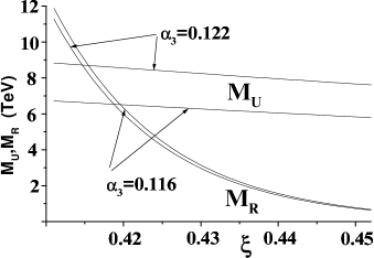
Figure 1: The scales $M_{U}$ and $M_{R}$ vs the parameter $\xi$. The requirements 1TeV$<M_{R}<M_{U}$ sets the range for $\xi$. The particle content has $n_{d^{c}_{H}}=0$ (see text).

In Fig.(1) we plot $M_{U}$ and $M_{R}$ vs $\xi$. The upper line for $M_{U}$ and the lower line for $M_{R}$ correspond to the highest acceptable value for $\alpha_{3}$ (with the other lines corresponding to the lowest value). The maximum range for the gauge coupling ratio $\xi$ at $M_{U}$ is $\xi\sim(0.413,0.445)$. At the lowest value both scales are of the order of 9.3TeV while at the highest $M_{U}\sim 8$TeV. In the case of absence of non-standard particles, the region of $\xi$ is $(0.415,0.445)$ and the corresponding values for the scales are 8.7 TeV and 7.8 TeV. We have also checked that the gauge couplings stay well in the perturbative region.

We further observe that the $M_{R}$ and $M_{U}$ scales merge for the lower $\xi$ values. Since consistency of the scale hierarchy demands $M_{R}\leq M_{U}$, this implies that there is a lower acceptable value of $\xi$ or a higher $M_{U}$ scale as Fig.(1) shows. On the other hand, experimental bounds on right handed bosons imply $M_{R}\gtrsim 1$TeV, this sets the upper bound on $\xi$ or equivalently, the lower bound on $M_{U}$.

4 The Supersymmetric Model

In this section we repeat the above analysis for the supersymmetric version of the model, where we need the extra Higgs representation

$$H=(\mathbf{4},1,2;1,0,\gamma)\rightarrow u_{H}(\mathbf{3},\mathbf{1},\frac{2}{3})+d_{H}(\mathbf{\bar{3}},\mathbf{1},-\frac{1}{3})+e_{H}(\mathbf{1},\mathbf{1},-1)+\nu_{H}(\mathbf{1},\mathbf{1},0)$$ (9)

The charge $\gamma$ is not fully constrained (as opposed to the case of $\bar{H}$) and, in principle, can take two values $\gamma=\pm 1$. However, if supersymmetry is assumed, as the corresponding charge of the field $\bar{H}$ has been determined to $\delta=-1$, the value of $\gamma$ should be fixed to $\gamma=1$. Further, the following exotic representations could appear

$$\begin{split}\bar{D}(\mathbf{6},\mathbf{1},\mathbf{1};-2,0,0)\\ h_{L}(\mathbf{1},\mathbf{1},\mathbf{2};0,1,0)\\ \bar{h}_{L}(\mathbf{1},\mathbf{1},\mathbf{2};0,-1,0)\\ \bar{h}_{R}(\mathbf{1},\mathbf{1},\mathbf{2};0,0,-1)\end{split}$$ (10)

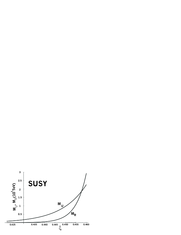
Figure 2: The scales $M_{U}$ and $M_{R}$ vs the parameter $\xi$ for the supersymmetric model, ($\gamma=1$, $\delta=-1$). The requirements for the scales are as in Fig.(1). The particle content is the minimum one (see text).

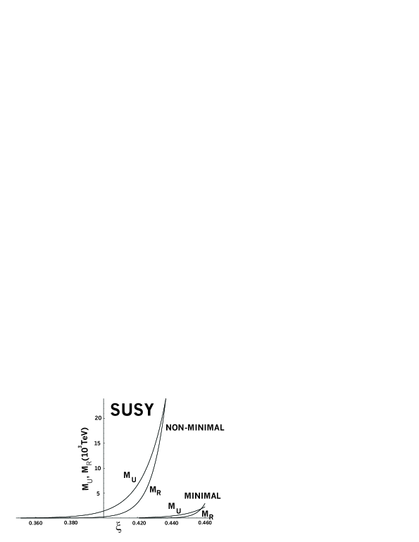
Figure 3: The scales $M_{U}$ and $M_{R}$ vs the parameter $\xi$ for the supersymmetric model for the minimal and a non minimal content.

Keeping the same conditions as in the non-supersymmetric case, Eqs(6,7) and fixing again the value of $c$ to $1/2$, we plot $M_{U}$ and $M_{R}$ vs $\xi$ in Fig.(2). The content is the minimum possible, i.e.

$$\begin{split}&n_{g}=3,\quad\quad n_{H}=1,\quad\quad n_{\bar{H}}=1,\quad\quad n_{h}=1,\quad\quad n_{D}=0,\quad\quad\\ &n_{\eta}=0,\quad\quad n_{h_{L}}=0\quad\quad n_{h_{R}}=0\\ &n_{H_{u}}=n_{H_{d}}=1,\quad\quad n_{d^{c}_{H}}=0,\quad\quad n_{\tilde{d}}=n_{\tilde{d}^{c}}=0\end{split}$$

We observe that, in contrast to the non-supersymmetric case examined in the previous section, here the limiting case $M_{R}=M_{U}$ is realized at the highest $\xi$ value, while the lower $\xi$ is correlated to the lower acceptable $M_{R}$ value ($\sim 1$ TeV). The energy scale of $M_{U}$ and $M_{R}$ now is three orders of magnitude higher than the corresponding non-supersymmetric case.

In Fig.(3) we show the same graph for the minimal and a non minimal content for the supersymmetric case ($\gamma=1$ and $\delta=-1$). The non minimal content drives the $\xi$ parameter to lower values but expands the acceptable region of the scales by almost one order of magnitude.

5 Yukawa Coupling Running for Top and Bottom

In the PS model with the minimal Higgs content, the Yukawa couplings for the top and the bottom quarks are equal at $M_{R}$, i.e. $h_{t}=h_{b}$. In this section we check whether such a constraint is compatible with the bottom and top quark masses as they are measured by the experiments. If $v_{1}$ and $v_{2}$ are the two v.e.v.’s that correspond to $H_{d}$ and $H_{u}$, we have of course:

$$m_{t}(m_{t})=h_{t}(m_{t})v_{2},\quad\quad m_{b}(m_{b})=h_{b}(m_{t})v_{1}\eta$$

where the factor $\eta=1.4$ takes care for the QCD renormalisation effects from the scale $m_{t}$ down to the mass of the bottom quark. Since we have two v.e.v.’s (although we do not have supersymmetry), the relation with $M_{Z}$ is:

$$M_{Z}=\frac{1}{2}\sqrt{g^{2}_{2}+g_{Y}^{2}}\,(v_{1}^{2}+v_{2}^{2})=\frac{1}{2}\sqrt{g^{2}_{2}+g_{Y}^{2}}\,v$$

while we insert, as usual, the parameter $\tan\beta=v_{2}/v_{1}$. The RGE for the two couplings are:

$$\begin{split}16\pi^{2}\frac{dh_{t}}{dt}&=h_{t}\left[\frac{3}{2}h_{t}^{2}-\frac{3}{2}h_{b}^{2}-4\pi\left(\frac{17}{12}\alpha_{Y}+\frac{9}{4}\alpha_{2}+8\alpha_{3}\right)\right]\\ 16\pi^{2}\frac{dh_{b}}{dt}&=h_{b}\left[\frac{3}{2}h_{b}^{2}-\frac{3}{2}h_{t}^{2}-4\pi\left(\frac{5}{12}\alpha_{Y}+\frac{9}{4}\alpha_{2}+8\alpha_{3}\right)\right]\\ \end{split}$$ (11)

where we have ignored all other Yukawa couplings. We run the equations from $M_{R}$ down to scale $M$ where $h_{t}(M)v_{2}=M$, which is the top mass $m_{t}$.

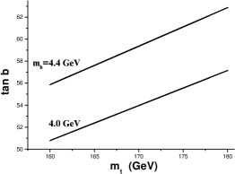
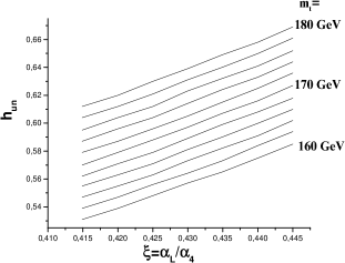
(a)	(b)

Figure 4: (a) The top mass vs $\tan b$ giving $m_{b}$ in the experimental range $(4.0-4.4)$GeV and (b) the parameter $\xi=\alpha_{L}/\alpha_{4}$ vs $h(M_{R})$ for several values of $m_{t}$.

In Fig(4a) we plot $m_{t}$ vs $\tan\beta$ in order to have $m_{b}$ in the acceptable experimental region (4.0-4.4)GeV. The choice of $\xi$ (in the acceptable region defined above) makes a very small effect which shows itself in the thickness of the lines. Since we require unification of the two Yukawa couplings at $M_{R}$, the large difference in the mass of the two quarks can only be provided by a large angle, therefore the large values of $\tan\beta$ were expected. Moreover, being in the large $\tan\beta$ regime, $m_{t}$ changes by a negligible amount as $\tan\beta$ changes to comply with the upper and lower limits of the bottom mass (remember that $v_{2}=v\sin b$ while $v_{1}=v\cos b$).

The form of the Eq.(11) also shows that the two couplings run almost “parallel” to each other and actually the main contribution to the running comes from the gauge couplings (as we can see in the next figure, the value of the Yukawas at $M_{R}$ are small). The corresponding figure with $n_{d^{c}_{H}}=2$ does not show any significant difference.

In Fig.(4b) we plot the parameter $\xi$ versus the unified value of the Yukawa coupling at $M_{R}$, for different values of $m_{t}$. The dependence is almost linear with higher value of $m_{t}$ requiring higher values of the unified Yukawa coupling $h$. The absolute value of the Yukawa coupling justifies our previous claim that the running of $h_{b}$ and $h_{t}$ is governed by the gauge coupling contributions to the RGE equations.

The last figure, Fig.(5), correspond to the supersymmetric case. The $\tan\beta$ vs $m_{t}$ figure does not show any significant difference from the corresponding non-supersymmetric case. On the contrary, the $h(M_{R})$ vs $\xi$ is different. Lower $\xi$ values corresponds to higher $h(M_{R})$ ones while the range of the acceptable $h(M_{R})$ values is a bit broader.

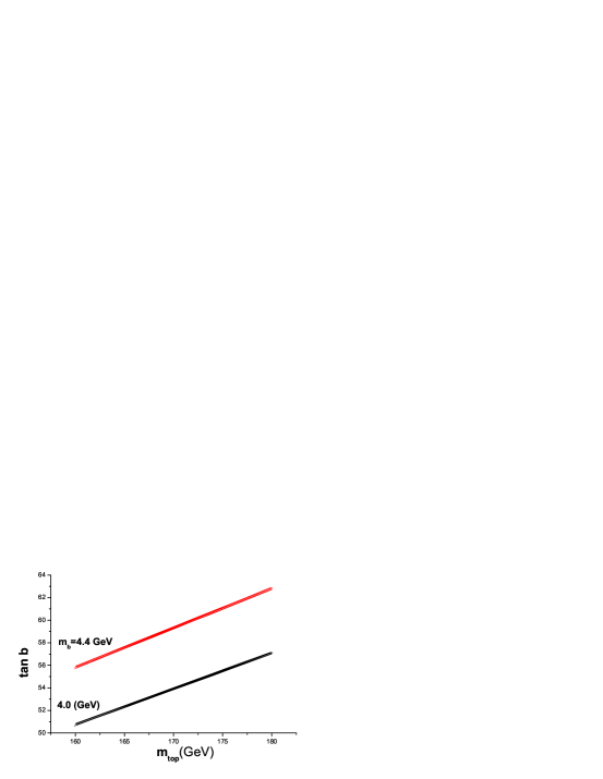
(a)	(b)

Figure 5: The SUSY case: (a) The top mass vs $\tan\beta$ giving $m_{b}$ in the experimental range $(4.0-4.4)$GeV and (b) The parameter $\xi=\alpha_{L}/\alpha_{4}$ vs $h(M_{R})$.

Finally, in figure (5 we plot the unified value of the Yukawa coupling $h_{u}$ versus the $\xi$ parameter. We note that, -in contrast to the non-supersymmetric case which is exhibited in figure (5)- here higher $h_{u}$ values are obtained for lower ratios $\xi$.

6 Conclusions

In the present work, we have examined the gauge and $bottom-top$ Yukawa coupling evolution in models with Pati-Salam symmetry obtained in the context of brane scenarios. In the case of ‘petit’ unification of gauge couplings, i.e., $a_{4}=a_{R}\neq a_{L}$, it turns out that in the non-supersymmetric version of the above model one may have a string scale at a few TeV. Further, assuming $h_{b}-h_{t}$ Yukawa unification at the string scale, one finds that the correct $m_{b,t}$ quark masses are obtained for a $a_{4}$ approximately twice as big as $a_{L}$. A similar analysis for the supersymmetric case shows that the string scale raises up to $10^{7}TeV$ while $h_{b}-h_{t}$ unification reproduces also the right mass relations $m_{b},m_{t}$.

We would like to thank G. Leontaris for valuable discussions and useful remarks and J. Rizos for helpful discussions.

References

- [1] I. Antoniadis, Phys. Lett. B 246 (1990) 377.
- [2] N. Arkani-Hamed, S. Dimopoulos and G. R. Dvali, Phys. Lett. B 429 (1998) 263 [arXiv:hep-ph/9803315].
- [3] I. Antoniadis, N. Arkani-Hamed, S. Dimopoulos and G. R. Dvali, Phys. Lett. B 436 (1998) 257 [arXiv:hep-ph/9804398].
- [4] J. D. Lykken, Phys. Rev. D 54 (1996) 3693 [arXiv:hep-th/9603133].
- [5] M. Berkooz, M. R. Douglas and R. G. Leigh, Nucl. Phys. B 480 (1996) 265 [arXiv:hep-th/9606139].
- [6] V. Balasubramanian and R. G. Leigh, Phys. Rev. D 55 (1997) 6415 [arXiv:hep-th/9611165].
- [7] G. Aldazabal, L. E. Ibanez and F. Quevedo, JHEP 0002 (2000) 015 [arXiv:hep-ph/0001083].
- [8] I. Antoniadis, E. Kiritsis and T. Tomaras, Fortsch. Phys. 49 (2001) 573 [arXiv:hep-th/0111269].
- [9] I. Antoniadis, E. Kiritsis and T. N. Tomaras, Phys. Lett. B 486 (2000) 186 [hep-ph/0004214].
- [10] I. Antoniadis, E. Kiritsis, J. Rizos and T. N. Tomaras, [arXiv:hep-th/0210263].
- [11] G. K. Leontaris and J. Rizos, Phys. Lett. B 510 (2001) 295 [arXiv:hep-ph/0012255].
- [12] C. Kokorelis, JHEP 0208 (2002) 036 [arXiv:hep-th/0206108].
- [13] I. Antoniadis, E. Kiritsis and J. Rizos, Nucl. Phys. B 637 (2002) 92 [arXiv:hep-th/0204153].
- [14] J. C. Pati and A. Salam, Phys. Rev. D 10 (1974) 275.
- [15] H. Dreiner, G.K. Leontaris, S. Lola, G.G. Ross and C. Scheich, Nucl. Phys. B436 (1995) 461 [arXiv:hep-ph/9409369].
- [16] M. K. Parida and A. Usmani, Phys. Rev. D 54 (1996) 3663.