Nonfactorizable corrections to $B\rightarrow J/\psi K$

Abstract

We apply the method of QCD light-cone sum rules to calculate nonfactorizable contributions to the $B\rightarrow J/\psi K$ decay and estimate soft nonfactorizable corrections to the $a_{2}$ parameter. The corrections appear to be positive, favoring the positive sign of $a_{2}$, in agreement with recent theoretical considerations and experimental data. Our result also confirms expectations that in the color-suppressed decay nonfactorizable corrections are sizable.

I Introduction

In nonleptonic decays of a $B$ meson one can study effects of hadronization, perturbative as well as nonperturbative dynamics, final state interaction effects and CP violation. Measurements of exclusive nonleptonic $B$ decays have reached sufficient precision to challenge our theoretical knowledge on such decays. It became clear that calculations have to reduce their theoretical uncertainties in order to make real use of data. Nowadays there exist several approaches which shed more light on the dynamical background of exclusive nonleptonic decays. The most exploited ones are QCD factorization BBNS and PQCD approach KLS . The PQCD model assumes that the two-body nonleptonic amplitude is perturbatively calculable if the Sudakov suppression is implemented to the calculation. In QCD factorization one can show the factorization of the weak decay amplitude at the leading order $1/m_{b}$ level and can consider systematically perturbatively calculable nonleading terms of $1/m_{b}$ expansion. None of these approaches can take nonperturbative ${\cal O}(1/m_{b})$ terms into account, but there is no evidence that such terms are negligible.

The $B\rightarrow J/\psi K$ decay is interesting because of the several reasons. There is a large discrepancy between the experiment and the (naive) factorization prediction. The naive factorization is based on the assumption that the nonleptonic amplitude (obtained in terms of matrix elements of four-quark operators by using the effective weak Hamiltonian) can be expressed as a product of matrix elements of two hadronic (bilinear) currents. It also predicts vanishing matrix elements of four-quark operators with the mismatch of the color indices. The naive factorization hypothesis has been confirmed experimentally only for class-I $B\to D^{(*)}M$ $(M=\pi,\rho,a_{1},D_{s},D_{s}^{*})$ decays. On the other hand, $B\rightarrow J/\psi K$ is the color-suppressed (class-II) decay and therefore a significant impact of nonfactorizable contributions is expected.

Effects of a violation of the factorization hypothesis in the $B\rightarrow J/\psi K$ mode have been, up to now, calculated by using different theoretical methods, resulting in the sign ambiguity of the decay amplitude i.e. $a_{2}$ parameter ($a_{2}$ parameter is the effective coefficient of four-quark operators in the weak Hamiltonian; it is defined below by eqs. (14) and (15)). The QCD sum rule approach KR2 predicted a negative value for $a_{2}$, while the PQCD hard scattering approach LY and the calculation done in QCD factorization Cheng gave the positive value for the $a_{2}$ parameter. Moreover, a detailed analysis of the experimentally determined $B$ meson branching ratios, although by assuming the universality of the $a_{2}$ parameter, gives conclusive evidence that generally the $a_{2}$ parameter should be positive NS . On the contrary, the negative value of $a_{2}$ would indicate that the $1/N_{c}$ term and the nonfactorizable part in the amplitude tend to cancel and would therefore confirm the large $N_{c}$ hypothesis BGR . The validity of this hypothesis was established in two-body $D$ meson decays, while, up to now, different attempts failed to prove this assumption for $B$ decays (see i.e discussion in KR1 ). However, the sign ambiguity of $a_{2}$ cannot be solved experimentally by considering the $B\rightarrow J/\psi K$ decay alone. One of the possibilities is to consider the interference between the short- and long-distance contributions to $B\rightarrow Kl^{+}l^{-}$ Soares .

Nonfactorizable corrections due to the exchange of hard gluons were calculated at $O(\alpha_{s})$ in QCD factorization. In this paper we concentrate on the LCSR estimation of soft nonfactorizable contributions in the $B\rightarrow J/\psi K$ decay coming from the exchange of soft gluons between the $J/\psi$ and the kaon. The calculation is based on the light-cone sum rules (LCSR) method Khodja . This method enables a consistent calculation of nonperturbative corrections of hadronic amplitudes inside the same framework reducing therefore the model uncertainties.

The paper is structured as follows. First, we discuss the results of the (naive) factorization method in Section II. The LCSR for the $B\rightarrow J/\psi K$ decay is derived in Section III. Next, to show the consistency of the method, we prove the factorization of the leading order contribution in Section IV. In Section V, the calculation of the soft nonfactorizable corrections is done by including twist-3 and twist-4 contributions. Section VI assembles the numerical results. In Section VII, using the results of calculation, we discuss impact of the nonfactorizable term on the factorization assumption and the implications of the results. A conclusion is given in Section VIII.

II Factorization hypothesis and nonfactorizable contributions

The part of the effective weak Hamiltonian relevant for the $B\rightarrow J/\psi K$ decay can be written in the form

$$H_{W}=\frac{G_{F}}{\sqrt{2}}V_{cb}V_{cs}^{*}\left[C_{1}(\mu){\cal O}_{1}+C_{2}(\mu){\cal O}_{2}\right]\,,$$ (1)

which can be further expressed as

$$H_{W}=\frac{G_{F}}{\sqrt{2}}V_{cb}V_{cs}^{*}\left[\left(C_{2}(\mu)+\frac{C_{1}(\mu)}{3}\right){\cal O}_{2}+2C_{1}(\mu){\cal\tilde{O}}_{2}\right]\,$$ (2)

where

$${\cal O}_{2}=(\overline{c}\Gamma_{\mu}c)(\overline{s}\Gamma^{\mu}b)\;\;,{\cal\tilde{O}}_{2}=(\overline{c}\Gamma_{\mu}\frac{\lambda_{a}}{2}c)(\overline{s}\Gamma^{\mu}\frac{\lambda_{a}}{2}b)\,.$$ (3)

Here $\Gamma_{\mu}=\gamma_{\mu}(1-\gamma_{5})$, $V_{ij}$’s are CKM matrix elements and $\lambda^{a}$’s are $SU(3)$ color matrices. $C_{1}(\mu)$ and $C_{2}(\mu)$ are short-distance Wilson coefficients computed at the renormalization scale $\mu\sim O(m_{b})$. The ${\cal\tilde{O}}_{2}$ operator appears after the projection of the color-mismatched quark fields in ${\cal{O}}_{1}=(\overline{c}\Gamma_{\mu}b)(\overline{s}\Gamma^{\mu}c)$ to a color singlet state:

$${\cal{O}}_{1}=\frac{1}{N_{c}}{\cal{O}}_{2}+2{\cal\tilde{O}}_{2}\,.$$ (4)

The $1/N_{c}$ term is the origin of the factor $1/3$ in (2).

Under the assumption that the matrix element for the $B\rightarrow J/\psi K$ decay factorizes, the matrix element of the ${\cal\tilde{O}}_{2}$ operator vanishes because of the color conservation and the rest can written as

$$\langle J/\psi K|H_{W}|B\rangle = \frac{G_{F}}{\sqrt{2}}V_{cb}V_{cs}^{*}\left[C_{2}(\mu)+\frac{C_{1}(\mu)}{3}\right]$$ (5)

$$\times\langle J/\psi K|{\cal O}_{2}|B\rangle^{fact}\left[1+O(\alpha_{s})+O\left(\frac{\Lambda_{QCD}}{m_{b}}\right)\right]\,,$$

where the second and the third term represent hard and soft corrections to the factorizable amplitude, respectively.

The factorized matrix element of the operator ${\cal O}_{2}$ is given by

$$\langle J/\psi(p)K(q)|{\cal O}_{2}|B(p+q)\rangle^{fact} = \langle J/\psi(p)|\overline{c}\Gamma_{\mu}c|0\rangle\langle K(q)|\overline{s}\Gamma^{\mu}b|B(p+q)\rangle$$ (6)

$$= 2\epsilon\cdot q\,m_{J/\psi}f_{J/\psi}F^{+}_{BK}(m_{J/\psi}^{2})\,$$

where meson momenta are explicitly specified and $p^{2}=m_{J/\psi}^{2}$. The $J/\psi$ decay constant is defined by the relation

$$\langle J/\psi(p)|\overline{c}\gamma_{\mu}c|0\rangle=f_{J/\psi}m_{J/\psi}\,\epsilon_{\mu}$$ (7)

with $\epsilon_{\mu}$ being the $J/\psi$ polarization vector which satisfies the condition $\epsilon\cdot p=0$. The $f_{J/\psi}$ denotes the $J/\psi$ decay constant determined by the experimental leptonic width $\Gamma(J/\psi\rightarrow l^{+}l^{-})=5.26\pm 0.37\;{\rm keV}$ by using the leading order calculation:

$$f_{J/\psi}=405\pm 14\,{\rm MeV}\,.$$ (8)

The $F_{BK}^{+}$ form factor is defined through the decomposition

$$\langle K(q)|\overline{s}\gamma_{\mu}b|B(p+q)\rangle=(2q+p)_{\mu}F^{+}_{BK}(p^{2})+\frac{m_{B}^{2}-m_{K}^{2}}{q^{2}}p_{\mu}(-F^{+}_{BK}(p^{2})+F^{0}_{BK}(p^{2}))$$ (9)

and estimated from the light-cone sum rules BKR ; KRWWY has the value

$$F^{+}_{BK}(m_{J/\psi}^{2})=0.55\pm 0.05\,.$$ (10)

By neglecting corrections in (5), the (naive) factorization expression for the $B\rightarrow J/\psi K$ decay emerges. Taking into account the NLO Wilson coefficients calculated in the NDR scheme BBL for $\mu=\overline{m_{b}}(m_{b})=4.40{\rm\,GeV}$ and $\Lambda_{\overline{\rm MS}}^{(5)}=225\,{\rm MeV}$,

$$C_{1}(\overline{m_{b}}(m_{b}))=1.082\,\qquad C_{2}(\overline{m_{b}}(m_{b}))=-0.185$$ (11)

and using the $B$ meson lifetime $\tau(B^{\pm})=1.653\pm 0.28\,ps$, we obtain for the branching ratio in the naive factorization

$${\cal B}(B\rightarrow J/\psi K)^{fact}=3.3\cdot 10^{-4}\,,$$ (12)

with the uncertainties in the order of $30\%$. This has to be compared with the recent measurements exp

$${\cal B}(B^{+}\rightarrow J/\psi K^{+}) = (10.1\pm 0.3\pm 0.5)\cdot 10^{-4}\,,$$

$${\cal B}(B^{0}\rightarrow J/\psi K^{0}) = (8.3\pm 0.4\pm 0.5)\cdot 10^{-4}\,.$$ (13)

Obviously there is a large discrepancy between the naive factorization prediction (12) and the experiment.

Returning to the expression for the $B\rightarrow J/\psi K$ amplitude (5), the corrections are given as an expansion in $1/m_{b}$ and $\alpha_{s}$. Apart from the $O(\alpha_{s})$ corrections to the factorizable part, there are also nonfactorizable corrections, which can be, either due to a hard gluon exchange or due to a soft gluon exchange (denoted in (5) as O($\alpha_{s}$) or $O(\Lambda_{QCD}/m_{b})$ corrections, respectively) between $J/\psi$ and the $B-K$ system.

To be able to discuss the impact of the nonfactorizable terms, it is usual to parameterize the $\langle J/\psi K|H_{W}|B\rangle$ amplitude in terms of the $a_{2}$ parameter as NS ; KR1

$$\langle J/\psi K|H_{W}|B\rangle=\sqrt{2}\,G_{F}\,V_{cb}V_{cs}^{*}\,\epsilon\cdot q\,m_{J/\psi}f_{J/\psi}F_{BK}^{+}(m_{J/\psi}^{2})\,a_{2}\,.$$ (14)

The effective parameter $a_{2}$ is defined by

$$a_{2}=C_{2}(\mu)+\frac{C_{1}(\mu)}{3}+2C_{1}(\mu)\frac{\tilde{F}_{BK}^{+}(\mu)}{F_{BK}^{+}(m_{J/\psi}^{2})}\,.$$ (15)

The part proportional to the $\tilde{F}_{BK}^{+}$ represents the nonfactorizable contribution from the ${\cal\tilde{O}}_{2}$ operator

$$\langle J/\psi K|{\cal\tilde{O}}_{2}(\mu)|B\rangle=2\epsilon\cdot q\,m_{J/\psi}f_{J/\psi}\tilde{F}_{BK}^{+}(\mu^{2})$$ (16)

and $\tilde{F}_{BK}^{+}=0$ corresponds to the naive factorization result, Eq. (6).

Because there is no explicit $\mu$ dependence of matrix element (6), the $\mu$ dependence of $a_{2}$ needs to be canceled by the nonfactorizable term. The nonvanishing nonfactorizable part is also required in order to suppress the strong renormalization scheme dependence of the effective parameter $a_{2}$ Buras .

Using the parameterization (14) we can extract the $a_{2}$ coefficient from the experiment. From the measurements (13) one obtains

$$|a_{2}^{exp}|=0.29\pm 0.03\,,$$ (17)

with the undetermined sign of $a_{2}$.

On the other hand, with the NLO Wilson coefficients from (11), the naive factorization yields

$$a_{2,\,NLO}^{fact}=C_{2}(m_{b})+\frac{C_{1}(m_{b})}{3}=0.176\,,$$ (18)

which is significantly below the value extracted from the experiment.

Following KR1 , in Fig.1 we show the partial width for $B\rightarrow J/\psi K$ as a function of the nonfactorizable amplitude $\tilde{F}_{BK}$.

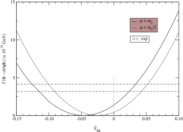
Figure 1: The partial width $\Gamma(B\rightarrow J/\psi K)$ as a function of the nonfactorizable amplitude $\tilde{F}_{BK}$.

The zero value of $\tilde{F}_{BK}$ corresponds to the factorizable prediction. There exist two ways to satisfy the experimental demands on the $\tilde{F}_{BK}$. According to the large $1/N_{c}$ rule assumption BGR , one can argue that there is a cancellation between $1/N_{c}$ piece of the factorizable part and the nonfactorizable contribution, (15). That would demand relatively small and negative value of $\tilde{F}_{BK}$. The other possibility is to have even smaller, but positive values for $\tilde{F}_{BK}$, which then compensate the overall smallness of the factorizable part and bring the theoretical estimation of $a_{2}$ in agreement with experiment.

One can note significant $\mu$ dependence of the theoretical expectation for the partial width in Fig.1, which brings an uncertainty in the prediction for $\tilde{F}_{BK}(\mu)$ of the order of $30\%$. This uncertainty is even more pronounced for the positive solutions of $\tilde{F}_{BK}(\mu)$. The values for $\tilde{F}_{BK}^{+}$ extracted from experiments

$$\tilde{F}_{BK}^{+}(m_{b}) = 0.028\qquad{\rm or}\qquad\tilde{F}_{BK}^{+}(m_{b})=-0.120\,,$$

$$\tilde{F}_{BK}^{+}(m_{b}/2) = 0.046\qquad{\rm or}\qquad\tilde{F}_{BK}^{+}(m_{b}/2)=-0.095\,.$$ (19)

clearly illustrate the $\mu$ sensitivity of the nonfactorizable part.

In the following we will calculate the nonfactorizable contribution $\tilde{F}_{BK}^{+}$, which appears due to the exchange of soft gluons, by using the QCD light-cone sum rule method.

III Light-cone sum rule for $\langle J/\psi K|{\cal O}|B\rangle$

III.1 The correlator

To estimate the soft-gluon exchange contributions to $B\rightarrow J/\psi K$ we use the method developed in Khodja for the $B\rightarrow\pi\pi$ case. In this approach one considers the correlation function:

$$F_{\nu}(p,q,k)=i^{2}\,\int d^{4}xe^{-i(p+q)x}\int d^{4}ye^{i(p-k)y}\langle K(q)|T\{j_{\nu}^{J/\psi}(y){\cal O}(0)j_{5}^{B}(x)\}|0\rangle\,,$$ (20)

where $j_{\nu}^{J/\psi}=\overline{c}\gamma_{\nu}c$ and $j_{5}^{B}=m_{b}\overline{b}i\gamma_{5}u$ are currents interpolating the $J/\psi$ and $B^{-}$ meson fields, respectively.

Figure 2: $B\rightarrow J/\psi K$ decay in LCSR. The shaded oval region denotes nonperturbative input, the $K$ meson light-cone distribution amplitude. $J/\psi$ and the $B$ meson are represented by the currents $j^{J/\psi}(p-k)$ and $j^{B}(p+q)$, respectively. The square stands for the ${\cal O}_{i}$ four-quark weak operators.

The correlator is a function of three independent momenta, chosen by convenience to be $q$, $p-k$ and $k$. Diagrammatically the correlator is shown in Fig.2.

Here, it is important to emphasize the role of the unphysical $k$ momentum in the weak vertex. It was introduced in order to avoid that the $B$ meson four-momenta before ($p_{B}$) and after the decay ($P$) are the same, Fig.2. In such a way, one avoids a continuum of light contributions in the dispersion relation in the $B$-channel. These contributions, like $D\overline{D}^{*}_{s}$ or $D^{*}\overline{D}_{s}$, have masses much smaller than the ground state $B$ meson mass and spoil the extraction of the physical $B$ state. Also, they are not exponentially suppressed by the Borel transformation (see for example the discussion in BS ).

The correlator (20) for nonvanishing $k$ is a function of 6 independent kinematical invariants. Four of them are taken to be the external momenta squared: $(p+q)^{2}$, $(p-k)^{2}$, $q^{2}$ and $k^{2}$, and additionally we take $P^{2}=(p-k+q)^{2}$ and $p^{2}$. We neglect the small corrections of the order $O(m_{K}^{2}/m_{B}^{2})$ and take $q^{2}=m_{K}^{2}=0$. Also, we set $k^{2}=0$. The $p^{2}$ momentum is for the moment kept undefined, in order to be able to make unrestricted derivation of the sum rules. Its value is going to be set later, by considering the twist-2 calculation of the factorizable part, Section IV, and will be chosen $p^{2}=m_{J/\psi}^{2}$ in order to reproduce the factorization result, (6). Furthermore, we take $(p-k)^{2}$, $(p+q)^{2}$ and $P^{2}$ spacelike and large in order to stay away from the hadronic thresholds in both, the $J/\psi$ and the $B$ channel. All together we have

$$q^{2}=k^{2}=0,\;p^{2}=m_{J/\psi}^{2},\;|(p-k)|^{2}\gg\Lambda_{QCD},|(p+q)|^{2}\gg\Lambda_{QCD},|P|^{2}\gg\Lambda_{QCD}\,.$$ (21)

III.2 Derivation

The first step is the derivation of the dispersion relation from the correlator (20). Inserting a complete set of hadronic states with the $J/\psi$ quantum numbers between the $J/\psi$ current and the weak operator in (20) gives us the following:

$$F_{\nu} = \frac{m_{J/\psi}f_{J/\psi}}{m_{J/\psi}^{2}-(p-k)^{2}}\sum_{\lambda}\epsilon_{\nu}^{\ast(\lambda)}\Pi((p+q)^{2},P^{2},p^{2},\epsilon^{(\lambda)}\cdot q_{i})$$ (22)

$$+ \int_{s_{0}^{h(J/\psi)}}^{\infty}ds\frac{\rho_{h\,,\nu}^{J/\psi}(s,(p+q)^{2},P^{2},p^{2})}{s-(p-k)^{2}}\,,$$

where $q_{i}=p,q,k$ and $\epsilon^{(\lambda)}\cdot(p-k)=0$. The sum runs over the polarizations of $J/\psi$. The lowest state contribution satisfies

$$\langle 0|\overline{c}\gamma_{\nu}c|J/\psi(p-k,\epsilon^{(\lambda)})\rangle=m_{J/\psi}f_{J/\psi}\epsilon^{\ast(\lambda)}_{\nu}$$ (23)

and $(p-k)^{2}=m_{J/\psi}^{2}$. In (22), $\rho_{h\,,\nu}^{J/\psi}$ and $s_{0}^{h(J/\psi)}$ are the spectral density and the threshold mass squared of the lowest excited resonances and continuum states of the $J/\psi$ channel, respectively.

The hadronic matrix element of interest is denoted by

$$\Pi((p+q)^{2},P^{2},p^{2},\epsilon^{(\lambda)}\cdot q_{i})=i\int d^{4}xe^{-i(p+q)x}\langle J/\psi(p-k,\epsilon^{(\lambda)})K(q)|T\{{\cal O}(0)j_{5}^{B}(x)\}|0\rangle\,.$$ (24)

On the other hand, for spacelike $(p-k)^{2}\ll m_{J/\psi}^{2}$ far away from the poles associated with the resonances and continuum states, the correlator $F_{\nu}$ can be calculated in QCD in terms of the quark and gluon degrees of freedom and written in a form of a dispersion relation as:

$${\cal F}_{\nu}=\frac{1}{\pi}\int_{4m_{c}^{2}}^{\infty}ds\frac{{\rm Im}_{s}{\cal F}_{\nu}(s,(p+q)^{2},P^{2},p^{2})}{s-(p-k)^{2}}\,,$$ (25)

with the kinematical decomposition

$${\cal F}_{\nu}=(p-k)_{\nu}F^{(p-k)}+k_{\nu}F^{(k)}+q_{\nu}F^{(q)}+\epsilon_{\nu\alpha\beta\gamma}(p-k)^{\alpha}k^{\beta}q^{\gamma}F^{(\epsilon)}\,.$$ (26)

By assuming quark-hadron duality one substitutes the hadronic spectral density $\rho_{h,\nu}^{J/\psi}$ in (22) with the one calculable in QCD and replaces $s_{0}^{h{(J/\psi)}}$ with the effective threshold of the perturbative continuum, $s_{0}^{J/\psi}$, i.e :

$$\rho_{h\,,\nu}^{J/\psi}(s,(p+q)^{2},P^{2},p^{2})\Theta(s-s_{0}^{h{(J/\psi)}})=\frac{1}{\pi}{\rm Im}_{s}{\cal F}_{\nu}(s,(p+q)^{2},P^{2},p^{2})\Theta(s-s_{0}^{J/\psi})\,.$$ (27)

By matching the hadronic relation (22) with the QCD calculation (25) one obtains the sum rule expression

$$\frac{m_{J/\psi}f_{J/\psi}}{m_{J/\psi}^{2}-(p-k)^{2}}\sum_{\lambda}\epsilon_{\nu}^{\ast(\lambda)}\Pi((p+q)^{2},P^{2},p^{2},\epsilon^{(\lambda)}\cdot q_{i}) =$$ (28)

$$\frac{1}{\pi}\int_{4m_{c}^{2}}^{s_{0}^{J/\psi}}ds\frac{{\rm Im}_{s}{\cal F}_{\nu}(s,(p+q)^{2},P^{2},p^{2})}{s-(p-k)^{2}}\,.$$

In order to reduce the impact of the approximation (27) and to suppress contributions from excited and continuum states, as usually done for quarkonium systems one performs $n$ derivations in the momentum $(p-k)^{2}$ and receives $n$-moment sum rule for the correlator $\Pi((p+q)^{2},P^{2},p^{2},\epsilon^{(\lambda)}\cdot q_{i})$ of the form

$$\sum_{\lambda}\epsilon_{\nu}^{\ast(\lambda)}\Pi((p+q)^{2},P^{2},p^{2},\epsilon^{(\lambda)}\cdot q_{i}) =$$ (29)

$$\frac{1}{\pi\,m_{J/\psi}f_{J/\psi}}\int_{4m_{c}^{2}}^{s_{0}^{J/\psi}}ds\frac{(m_{J/\psi}^{2}+Q_{0}^{2})^{n+1}}{(s+Q_{0}^{2})^{n+1}}{\rm Im}_{s}{\cal F}_{\nu}(s,(p+q)^{2},P^{2},p^{2})\,,$$

where $Q_{0}$ is the sum rule parameter that role will be discussed later, in Section VI.

We proceed by using the analytical properties of the $\Pi((p+q)^{2},P^{2},p^{2},\epsilon^{(\lambda)}\cdot q_{i})$ amplitude in the $(p+q)^{2}$ variable of the $B$-channel and insert in (24) the complete set of hadronic states with the $B$ meson quantum numbers which yields

$$\sum_{\lambda}\epsilon_{\nu}^{\ast(\lambda)}\Pi((p+q)^{2},P^{2},p^{2},\epsilon^{(\lambda)}\cdot q_{i}) =$$

$$\frac{m_{B}^{2}f_{B}}{m_{B}^{2}-(p+q)^{2}}\sum_{\lambda}\epsilon_{\nu}^{\ast(\lambda)}\langle J/\psi(p-k,\epsilon^{(\lambda)})K(q)|{\cal O}(0)|B(p+q)\rangle+\int_{s_{0}^{h(B)}}^{\infty}ds^{\prime}\frac{\rho_{h,\nu}^{B}(s^{\prime},P^{2},p^{2})}{s^{\prime}-(p+q)^{2}}\,.$$

In above, as before, it is assumed that in the last term the polarization sum is already done.

The QCD part, given by the r.h.s of the eq.(29) and rewritten in a form of the dispersion relation, now in the $(p+q)^{2}$ variable, exposes the form of the double dispersion relation as

$$\frac{1}{\pi}\int_{4m_{c}^{2}}^{s_{0}^{J/\psi}}ds\frac{(m_{J/\psi}^{2}+Q_{0}^{2})^{n+1}}{(s+Q_{0}^{2})^{n+1}}{\rm Im}_{s}{\cal F}_{\nu}(s,(p+q)^{2},P^{2},p^{2}) =$$ (31)

$$\frac{1}{\pi^{2}}\int_{4m_{c}^{2}}^{s_{0}^{J/\psi}}ds\frac{(m_{J/\psi}^{2}+Q_{0}^{2})^{n+1}}{(s+Q_{0}^{2})^{n+1}}\int_{m_{b}^{2}}^{f_{1}(s,P^{2},p^{2})}\frac{ds^{\prime}}{s^{\prime}-(p+q)^{2}}{\rm Im}_{s^{\prime}}{\rm Im}_{s}{\cal F}_{\nu}(s,s^{\prime},P^{2},p^{2})$$

From the Maldestam representation of the kinetic variables one can see that the integration limit of $s^{\prime}$ variable is going in general to depend on $s$, $P^{2}$ and $p^{2}$ and we denoted these dependence by $f_{1}(s,P^{2},p^{2})$. In the following, those terms which disappear after taking moments in $J/\psi$ channel and after making the Borel transform in the $B$-channel are neglected.

In order to subtract the continuum of $B$ states, we exchange the order of the integration in (31) and use quark-hadron duality in $B$ channel in a sense that the spectral density $\rho_{h}^{B}$ is approximated by the $s^{\prime}\geq s_{0}^{B}$ part of the double dispersion integral (31), where $s_{0}^{B}$ is the effective threshold of the perturbative continuum in the $B$ channel. Therefore,

$$\frac{m_{B}^{2}f_{B}}{m_{B}^{2}-(p+q)^{2}}\sum_{\lambda}\epsilon_{\nu}^{\ast(\lambda)}\langle J/\psi(p-k,\epsilon^{(\lambda)})K(q)|{\cal O}(0)|B(p+q)\rangle = \frac{1}{\pi^{2}\,m_{J/\psi}f_{J/\psi}}$$ (32)

$$\times\int_{4m_{c}^{2}}^{s_{0}^{J/\psi}}ds\frac{(m_{J/\psi}^{2}+Q_{0}^{2})^{n+1}}{(s+Q_{0}^{2})^{n+1}}\int_{m_{b}^{2}}^{f_{2}(s,s_{0}^{B},P^{2},p^{2})}\frac{ds^{\prime}}{s^{\prime}-(p+q)^{2}}{\rm Im}_{s^{\prime}}{\rm Im}_{s}{\cal F}_{\nu}(s,s^{\prime},P^{2},p^{2})$$

and after the Borel transformation in $(p+q)^{2}$ variable, we can further write

$$\sum_{\lambda}\epsilon_{\nu}^{\ast(\lambda)}\langle J/\psi(p-k,\epsilon^{(\lambda)})K(q)|{\cal O}(0)|B(p+q)\rangle = \frac{1}{\pi^{2}\,m_{J/\psi}f_{J/\psi}m_{B}^{2}f_{B}}$$ (33)

$$\times\int_{4m_{c}^{2}}^{s_{0}^{J/\psi}}ds\frac{(m_{J/\psi}^{2}+Q_{0}^{2})^{n+1}}{(s+Q_{0}^{2})^{n+1}}\int_{m_{b}^{2}}^{f_{2}(s,s_{0}^{B},P^{2},p^{2})}ds^{\prime}e^{(m_{B}^{2}-s^{\prime})/M^{2}}{\rm Im}_{s^{\prime}}{\rm Im}_{s}{\cal F}_{\nu}(s,s^{\prime},P^{2},p^{2})\,,$$

In above, $M$ is the Borel parameter and the function $f_{2}$ is the upper limit of the $s$ integral after subtraction of continuum of $B$ channel.

Further, to extract the kinematical structure of interests, we decompose the matrix element $\langle J/\psi(p-k,\epsilon^{(\lambda)})K(q)|{\cal O}(0)|B(p+q)\rangle$ as

$$\langle J/\psi(p-k,\epsilon^{(\lambda)})K(q)|{\cal O}(0)|B(p+q)\rangle = \epsilon\cdot q\,A^{(q)}+\epsilon\cdot k\,A^{(k)}$$ (34)

$$+\epsilon_{\alpha}\epsilon^{\alpha\rho\sigma\xi}(p-k)^{\rho}k^{\sigma}q^{\xi}\,A^{(\epsilon)}$$

By inserting this expansion in the expression (33), after the summation of the polarization vectors

$$\sum_{\lambda}\epsilon_{\nu}^{\ast(\lambda)}\epsilon_{\alpha}^{(\lambda)}=\left(-g_{\nu\alpha}+\frac{(p-k)_{\nu}(p-k)_{\alpha}}{(p-k)^{2}}\right)$$ (35)

one obtains the sum rule for different kinematical structures:

$$-k_{\nu}\;A^{(k)}-q_{\nu}\;A^{(q)}-\epsilon_{\nu\rho\sigma\xi}(p-k)^{\rho}q^{\sigma}k^{\xi}\;A^{(\epsilon)}$$

$$\hskip 14.22636pt+(p-k)_{\nu}\left(\frac{(p-k)\cdot k}{(p-k)^{2}}\;A^{(k)}+\frac{(p-k)\cdot q}{(p-k)^{2}}\;A^{(q)}\right)=$$

$$\hskip 8.5359pt=\frac{1}{\pi^{2}\,m_{J/\psi}f_{J/\psi}m_{B}^{2}f_{B}}\int_{4m_{c}^{2}}^{s_{0}^{J/\psi}}ds\frac{(m_{J/\psi}^{2}+Q_{0}^{2})^{n+1}}{(s+Q_{0}^{2})^{n+1}}\int_{m_{b}^{2}}^{f_{2}(s,s_{0}^{B},P^{2},p^{2})}ds^{\prime}e^{(m_{B}^{2}-s^{\prime})/M^{2}}$$

$$\hskip 19.91684pt\times{\rm Im}_{s^{\prime}}{\rm Im}_{s}\left[k_{\nu}\;F^{(k)}+q_{\nu}\;F^{(q)}+(p-k)_{\nu}F^{(p-k)}+\epsilon_{\nu\rho\sigma\xi}(p-k)^{\rho}q^{\sigma}k^{\xi}\;F^{(\epsilon)}\right]$$

$$\,.$$ (36)

The coefficient function in front of $(p-k)_{\nu}$ looks like

$$A^{(p-k)}=\left(\frac{(p-k)\cdot k}{(p-k)^{2}}\;A^{(k)}+\frac{(p-k)\cdot q}{(p-k)^{2}}\;A^{(q)}\right)\,,$$ (37)

which is a consequence of the conserved $J/\psi$ current. The sum rule expression for the $A^{(p-k)}$ part reads

$$A^{(p-k)} = \frac{1}{\pi^{2}\,m_{J/\psi}f_{J/\psi}m_{B}^{2}f_{B}}$$

$$\times\int_{4m_{c}^{2}}^{s_{0}^{J/\psi}}ds\frac{(m_{J/\psi}^{2}+Q_{0}^{2})^{n+1}}{(s+Q_{0}^{2})^{n+1}}\int_{m_{b}^{2}}^{f_{2}(s,s_{0}^{B},P^{2},p^{2})}ds^{\prime}e^{(m_{B}^{2}-s^{\prime})/M^{2}}{\rm Im}_{s^{\prime}}{\rm Im}_{s}\;F^{(p-k)}(s,s^{\prime},P^{2},p^{2})\,.$$

At the end we analytically continue $P^{2}$ to $P^{2}\geq 0$, and choose $P^{2}=m_{B}^{2}$. This enables the extraction of the physical matrix element, because the unphysical momentum $k$ disappears from the ground state contribution, due to the simultaneous conditions applied, $P^{2}=m_{B}^{2}$ and $(p+q)^{2}=m_{B}^{2}$. From (34) and (37) follows

$$\langle J/\psi(p,\epsilon^{(\lambda)})K(q)|{\cal O}(0)|B(p+q)\rangle=\epsilon\cdot q\,A^{(q)}(P^{2}=m_{B}^{2})=\epsilon\cdot q\frac{2p^{2}}{m_{B}^{2}-p^{2}}A^{(p-k)}(P^{2}=m_{B}^{2})$$ (39)

and the final sum rule relation for the physical matrix element $\langle J/\psi(p,\epsilon^{(\lambda)})K(q)|{\cal O}(0)|B(p+q)\rangle$ takes the form

$$\langle J/\psi(p,\epsilon^{(\lambda)})K(q)|{\cal O}(0)|B(p+q)\rangle =$$ (40)

$$=2\epsilon\cdot qm_{J/\psi}f_{J/\psi}\Bigg{\{}\frac{1}{\pi^{2}f_{J/\psi}^{2}}\int_{4m_{c}^{2}}^{s_{0}^{J/\psi}}ds\frac{(m_{J/\psi}^{2}+Q_{0}^{2})^{n+1}}{(s+Q_{0}^{2})^{n+1}}\frac{1}{m_{B}^{2}f_{B}}\int_{m_{b}^{2}}^{f_{2}(s,s_{0}^{B},m_{B}^{2},p^{2})}ds^{\prime}e^{(m_{B}^{2}-s^{\prime})/M^{2}}$$

$$\times\left[\frac{p^{2}}{\displaystyle m_{J/\psi}^{2}(m_{B}^{2}-p^{2})}\,{\rm Im}_{s^{\prime}}{\rm Im}_{s}F^{(p-k)}(s,s^{\prime},m_{B}^{2},p^{2})\right]\Bigg{\}}\,.$$

Some comments are in order. The $B\rightarrow J/\psi K$ case seems to be much more complicated than the decay of a $B$ meson to two light pions discussed in Khodja . The complication does not appear only due to the massive $c$ quarks, or the vector structure of the $J/\psi$ current, but mainly due to the local duality assumption in $J/\psi$ channel, which is expected to work much worse than in the pion channel in the $B\rightarrow\pi\pi$ decay. Although it is possible to stay away from the the excited and resonant hadronic states in the $J/\psi$ channel, one can still expect that there will be an influence of the $\psi^{\prime}$ resonance, which, in a more precise calculation has to be taken into account explicitly. The technical difficulties which are induced by the fact that the value of $P^{2}$ parameter is close to the hadronic threshold of $J/\psi$ are left for the discussion in Section V.

IV Factorization in the light-cone sum rule approach

We first consider the contribution of the ${\cal O}_{2}$ operator. As we have shown in the introduction, this operator contributes to the factorizable part of the matrix element $\langle J/\psi(p,\epsilon^{(\lambda)})K(q)|H_{W}|B(p+q)\rangle$.

The main contribution comes from the diagram shown in Fig.2, where for ${\cal O}={\cal O}_{2}$ there is no interaction between the charm loop and the $B-K$ system at the leading level. Therefore, the calculation of this contribution is rather simple. According to the expression (40), the $(p-k)_{\nu}$ part of the correlation function (20), $F^{(p-k)}$ needs to be calculated and its double imaginary part has to be extracted. The calculation proceeds in several steps. One inserts first explicitly the $J/\psi$ and $B$ currents in (20), and takes the expression (3) for the operator ${\cal O}_{2}$. The $c$-quarks are contracted to a $c\overline{c}$-loop and can be then independently integrated. The contraction of $b$-fields produces a free $b$-quark propagator and the rest of the fields is organized into the leading, twist-2 kaon distribution amplitude $\phi_{K}$. Explicitly, we obtain

$$F^{(p-k)}_{tw2}=\frac{m_{b}^{2}f_{K}}{4\pi^{2}}\int_{4m_{c}^{2}}^{\infty}\frac{ds}{s-(p-k)^{2}}q\cdot(p-k)\left(1+\frac{2m_{c}^{2}}{s}\right)\sqrt{1-\frac{4m_{c}^{2}}{s}}\int_{0}^{1}du\frac{\phi_{K}(u)}{m_{b}^{2}-(p+qu)^{2}}\,,$$ (41)

where $\phi_{K}(u)$ is the kaon twist-2 distribution amplitude defined by

$$\langle K(q)|\overline{s}(0)\gamma_{\mu}\gamma_{5}u(x)|0\rangle=-iq_{\mu}\,f_{K}\int_{0}^{1}due^{iuqx}\phi_{K}(u)\,.$$ (42)

The first integral in (41), apart from the kinematical factor $q\cdot(p-k)$, is nothing else but the charm loop contribution to the vacuum polarization calculated in the sum rule approach Reinders . The second integral, considered in the leading twist approximation, reduces exactly to the light-cone twist-2 expression for the $F_{BK}^{+}$ form factor BKR ; KRWWY . This part, with the substitution $u=(m_{b}^{2}-p^{2})/(s^{\prime}-p^{2})$, can be rewritten in a dispersion form as

$$\int_{0}^{1}du\frac{\phi_{K}(u)}{m_{b}^{2}-(p+qu)^{2}}=\int_{m_{b}^{2}}^{\infty}\frac{ds^{\prime}}{s^{\prime}-(p+q)^{2}}\frac{1}{s^{\prime}-p^{2}}\phi_{K}(u(s^{\prime}))\,.$$ (43)

In such a way the expression (41) receives the needed double dispersion form from which the double imaginary part in $s$ and $s^{\prime}$ variables can be trivially extracted.

The contribution of the ${\cal O}_{2}$ operator to the $B\rightarrow J\psi K$ matrix element then follows from the the sum rule relation (40):

$$\langle J/\psi(p,\epsilon^{(\lambda)})K(q)|{\cal O}_{2}(0)|B(p+q)\rangle_{tw2} =$$ (44)

$$=2\epsilon\cdot q\frac{m_{J/\psi}}{f_{J/\psi}}$$

$$\left[\frac{(m_{J/\psi}^{2}+Q_{0}^{2})^{n+1}}{4\pi^{2}}\int_{4m_{c}^{2}}^{s_{0}^{J/\psi}}\frac{ds}{(s+Q_{0}^{2})^{n+1}}\left(1+\frac{2m_{c}^{2}}{s}\right)\sqrt{1-\frac{4m_{c}^{2}}{s}}\frac{p^{2}}{m_{J/\psi}^{2}}\frac{\displaystyle(1-\frac{s}{m_{B}^{2}})}{\displaystyle(1-\frac{p^{2}}{m_{B}^{2}})}\right]$$

$$\times\left[\frac{f_{K}m_{b}^{2}}{2f_{B}m_{B}^{2}}\int_{m_{b}^{2}}^{s_{0}^{B}}\frac{ds^{\prime}}{s^{\prime}-p^{2}}e^{(m_{B}^{2}-s^{\prime})/M^{2}}\phi_{K}\left(\frac{m_{b}^{2}-p^{2}}{s^{\prime}-p^{2}}\right)\right]$$

$$\simeq 2\epsilon\cdot q\,m_{J/\psi}f_{J/\psi}F_{B\rightarrow K}^{+}(p^{2})\,.$$

Here we see that the amplitude $\langle J/\psi(p,\epsilon^{(\lambda)})K(q)|{\cal O}_{2}(0)|B(p+q)\rangle$ factorizes and in a good approximation the factorizable expression for the
$\langle J/\psi(p,\epsilon^{(\lambda)})K(q)|{\cal O}_{2}(0)|B(p+q)\rangle$ amplitude, given by (6), is recovered for $p^{2}=m_{J/\psi}^{2}$. In the first parenthesis, apart from the small $(1-s/m_{B}^{2})/(1-m_{J/\psi}^{2}/m_{B}^{2})$ correction, there is the leading order expression for the $f_{J/\psi}^{2}$ in the QCD sum rule approach. The correction is the result of calculation with the nonvanishing $k$ momentum. The second parenthesis in (44) gives the twist-2 contribution to $F_{BK}^{+}(p^{2})$ form factor. By reproducing the factorization result for $p^{2}=m_{J/\psi}^{2}$, we fix the value $p^{2}=m_{J/\psi}^{2}$ also in the further calculation.

V Soft nonfactorizable contributions in the LCSR approach

For a discussion of nonfactorizable contributions to the $B\rightarrow J/\psi K$ decay, we need to do a systematic $\alpha_{s}$ and twist expansion of the correlator (20).

After explicit insertion of the interpolating $J/\psi$ and $B$ meson currents and the operator ${\cal O}_{2}$ or $\tilde{\cal O}_{2}$, the correlation function (20) can be written in form:

$$F_{\nu}(p,q,k) = m_{b}\int d^{4}xe^{-i(p+q)x}\int d^{4}ye^{i(p-k)y}A^{jk}A^{lm}$$ (45)

$$\langle K(q)|Tr[\gamma_{\nu}S^{ij}(y,0|m_{c})\Gamma_{\mu}S^{ki}(0,y|m_{c})]\,\overline{s}^{l}\Gamma^{\mu}S^{mn}(0,x|m_{b})\gamma_{5}u^{n}|0\rangle\,,$$

where $i,j,k,l,m,n$ are color indices, $S(x,y|m)$ are quark propagators defined in (46) below and $A^{ij}=\delta^{ij}$ or $A^{ij}=T^{ij}=(\lambda^{a}/2)^{ij}$ for the insertion of ${\cal O}_{2}$ or $\tilde{\cal O}_{2}$ operator, respectively.

The $\alpha_{s}$ and twist expansion is achieved by considering the light-cone expression for quark propagators. Up to terms proportional to $G$, the propagation of a massive quark in the external gluon field in the Fock-Schwinger gauge is given by BK

$$S^{ij}(x_{1},x_{2}|m) \equiv -i\langle 0|T\{q^{i}(x_{1})\,\bar{q}^{j}(x_{2})\}|0\rangle$$ (46)

$$=\int\frac{d^{4}k}{(2\pi)^{4}}e^{-ik(x_{1}-x_{2})}\Bigg{\{}\frac{\not\!k+m}{k^{2}-m^{2}}\delta^{ij}-\int\limits_{0}^{1}dv\,g_{s}\,G^{\mu\nu}_{a}(vx_{1}+(1-v)x_{2})\left(\frac{\lambda^{a}}{2}\right)^{ij}$$

$$\times\Big{[}\frac{1}{2}\frac{\not\!k+m}{(k^{2}-m^{2})^{2}}\sigma_{\mu\nu}-\frac{1}{k^{2}-m^{2}}v(x_{1}-x_{2})_{\mu}\gamma_{\nu}\Big{]}\Bigg{\}}\,.$$

Figure 3: Soft nonfactorizable contributions to the correlation function (20).

From the above, considering the color structure of the ${\cal O}_{2}$ operator, we can easily deduce that the nonfactorizable contribution from this operator appears first at the two-gluon level and is therefore of $O(\alpha_{s}^{2})$. On the contrary, nonfactorizable corrections from the $\tilde{\cal O}_{2}$ operator are already given by the one-gluon exchange. The leading hard nonfactorizable contributions are due to the exchange of a hard gluon between the $c$-quark (antiquark) and the one of the remaining $b$, $\overline{u}$ or $s$ quarks, see Fig.2. These contributions emerge at the two-loop level and although they are calculable in LCSR, their calculation is technically very demanding and will not be discussed in this paper.

Insertion of the gluonic term of the propagator $S^{ij}(y,0,m_{c})$ or $S^{ki}(0,y,m_{c})$ yields the contributions represented in Fig.3. These are the leading soft nonfactorizable contributions. In terms of the light-cone expansion they are of the higher twist and described by the three particle kaon distribution amplitudes defined by the following matrix elements:
- twist-3 distribution amplitude

$$\langle 0|\overline{s}(0)\sigma_{\mu\nu}\gamma_{5}G_{\alpha\beta}(vy)u(x)|K^{+}(q)\rangle = if_{3K}\left[(q_{\alpha}q_{\mu}g_{\beta\nu}-q_{\beta}q_{\mu}g_{\alpha\nu})\right.$$ (47)

$$\left.-(q_{\alpha}q_{\nu}g_{\beta\mu}-q_{\beta}q_{\nu}g_{\alpha\mu})\right]\int{\cal D}\alpha_{i}\phi_{3K}(\alpha_{i},\mu)e^{-iq(x\alpha_{1}+yv\alpha_{3})}$$

- twist-4 distribution amplitudes

$$\langle 0|\overline{s}(0)i\gamma_{\mu}\tilde{G}_{\alpha\beta}(vy)u(x)|K^{+}(q)\rangle=q_{\mu}\frac{q_{\alpha}x_{\beta}-q_{\beta}x_{\alpha}}{qx}f_{K}\int{\cal D}\alpha_{i}\tilde{\phi}_{||}(\alpha_{i},\mu)e^{-iq(x\alpha_{1}+yv\alpha_{3})}$$

$$+(g_{\mu\alpha}^{\perp}q_{\beta}-g_{\mu\beta}^{\perp}q_{\alpha})\int{\cal D}\alpha_{i}\tilde{\phi}_{\perp}(\alpha_{i},\mu)e^{-iq(x\alpha_{1}+yv\alpha_{3})}$$ (48)

$$\langle 0|\overline{s}(0)\gamma_{\mu}\gamma_{5}{G}_{\alpha\beta}(vy)u(x)|K^{+}(q)\rangle=q_{\mu}\frac{q_{\alpha}x_{\beta}-q_{\beta}x_{\alpha}}{qx}f_{K}\int{\cal D}\alpha_{i}{\phi}_{||}(\alpha_{i},\mu)e^{-iq(x\alpha_{1}+yv\alpha_{3})}$$

$$+(g_{\mu\alpha}^{\perp}q_{\beta}-g_{\mu\beta}^{\perp}q_{\alpha})\int{\cal D}\alpha_{i}{\phi}_{\perp}(\alpha_{i},\mu)e^{-iq(x\alpha_{1}+yv\alpha_{3})}\,.$$ (49)

In above, $\tilde{G}_{\alpha\beta}=\frac{1}{2}\epsilon_{\alpha\beta\rho\sigma}G^{\rho\sigma}$, $G^{\rho\sigma}=g_{s}\,\lambda^{a}/2\,G^{\rho\sigma}_{a}$, ${\cal D}\alpha_{i}=d\alpha_{1}d\alpha_{2}d\alpha_{3}\delta(1-\alpha_{1}-\alpha_{2}-\alpha_{3})$, and $g_{\alpha\beta}^{\perp}=g_{\alpha\beta}-(x_{\alpha}q_{\beta}+x_{\beta}q_{\alpha})/qx$. Both twist-3 and twist-4 distribution amplitudes contribute at the same order. They are parameterized by

$$\phi_{3K}(\alpha_{i},\mu) = 360\alpha_{1}\alpha_{2}\alpha_{3}^{2}\left(1+a(\mu)\frac{1}{2}(7\alpha_{3}-3)+b(\mu)(2-4\alpha_{1}\alpha_{2}-8\alpha_{3}(1-\alpha_{3}))\right.$$ (50)

$$+\left.c(\mu)(3\alpha_{1}\alpha_{2}-2\alpha_{3}+3\alpha_{3}^{2})\right)\,,$$

$$\phi_{\perp}(\alpha_{i},\mu) = 30\delta^{2}(\mu)(\alpha_{1}-\alpha_{2})\alpha_{3}^{2}\left[\frac{1}{3}+2\epsilon(\mu)(1-2\alpha_{3})\right]\,,$$ (51)

$$\phi_{||}(\alpha_{i},\mu) = 120\delta^{2}(\mu)\epsilon(\mu)(\alpha_{1}-\alpha_{2})\alpha_{1}\alpha_{2}\alpha_{3}\,,$$ (52)

$$\tilde{\phi}_{\perp}(\alpha_{i},\mu) = 30\delta^{2}(\mu)\alpha_{3}^{2}(1-\alpha_{3})\left[\frac{1}{3}+2\epsilon(\mu)(1-2\alpha_{3})\right]\,,$$ (53)

$$\tilde{\phi}_{||}(\alpha_{i},\mu) = -120\delta^{2}(\mu)\alpha_{1}\alpha_{2}\alpha_{3}\left[\frac{1}{3}+\epsilon(\mu)(1-3\alpha_{3})\right]\,.\$$ (54)

The parameters are estimated from sum rules CZ ; BF and the values are listed in KR2 . In the numerical evaluation we use the asymptotic form of the above expressions where $a(\mu),b(\mu),c(\mu)$ and $\epsilon(\mu)$ dependence is neglected. The asymptotic expressions for twist-3 and twist-4 distribution amplitudes should provide sufficiently reliable estimates of already subleading contributions.

The QCD calculation of two diagrams in Fig.3 at the twist 3 level yields

$$F^{(p-k)}_{tw3} = -\frac{m_{b}f_{3K}}{4\pi^{2}}\int_{0}^{1}dv\int{\cal D}\alpha_{i}\frac{\phi_{3K}(\alpha_{i},\mu)}{m_{b}^{2}-(p+q(1-\alpha_{1}))^{2}}\,\int_{0}^{1}dx\frac{2x^{2}(1-x)}{m_{c}^{2}-\overline{Q}^{2}x(1-x)}$$ (55)

$$\times\,q\cdot(p-k)\Big{[}(2-v)q\cdot k+2(1-v)q\cdot(p-k)\Big{]}\,,$$

where $\overline{Q}=p-k+v\alpha_{3}q$. Comparing the above expression with the one obtained for the $B\rightarrow\pi\pi$ case, (Eq. (26) in Khodja ), we can see that there is an additional, $x$-integral for the massive $c\overline{c}$ loop. Otherwise, the expressions are the same and for $m_{c}\rightarrow 0$ the result form Eq. (26) in Khodja is exactly recovered, up to a sign, which can be traced back to a difference between the pseudoscalar and vector currents interpolating $\pi$ and $J/\psi$, respectively.

By changing the order and variables of integration one can bring the above expression into the following form:

$$F^{(p-k)}_{tw3} = \frac{m_{b}f_{3K}}{16\pi^{2}}\int_{4m_{c}^{2}}^{\infty}\frac{ds}{s-(p-k)^{2}}\int_{0}^{1-\frac{4m_{c}^{2}}{s}}\frac{dy}{2\sqrt{y}}\int_{x(s,y,P^{2})}^{1}\frac{du}{m_{b}^{2}-(p+qu)^{2}}$$ (56)

$$\times\int_{x(s,y,P^{2})}^{u}\frac{dv}{v^{2}}\phi_{3K}(1-u,u-v,v)$$

$$\hskip 28.45274pt\times\Big{[}s-\frac{4m_{c}^{2}}{1-y}+\left((p+q)^{2}-p^{2}\right)(2v-x(s,y,P^{2}))\Big{]}\,,$$

and

$$x(s,y,P^{2})=\frac{s-\frac{\displaystyle 4m_{c}^{2}}{\displaystyle 1-y^{2}}}{s-P^{2}}\,.$$ (57)

It is important to emphasize here that the above expression (56) is defined only for large spacelike momentum $|P^{2}|\sim m_{b}^{2}$. Furthermore, the expression (56) does not have a needed double dispersion form.

In order to proceed we write

$$F^{(p-k)}_{tw3} = \frac{1}{\pi}\int_{4m_{c}^{2}}^{\infty}\frac{ds}{s-(p-k)^{2}}{\rm Im_{s}}\,F_{tw3}^{(p-k)}(s,(p+q)^{2},P^{2},p^{2})\,,$$ (58)

where

$${\rm Im_{s}}\,F_{tw3}^{(p-k)}(s,(p+q)^{2},P^{2},p^{2}) =$$ (59)

$$\frac{m_{b}f_{3K}}{16\pi}\int_{0}^{1-\frac{4m_{c}^{2}}{s}}\frac{dy}{2\sqrt{y}}\int_{x(s,y,P^{2})}^{1}\frac{du}{m_{b}^{2}-(p+qu)^{2}}\int_{x(s,y,P^{2})}^{u}\frac{dv}{v^{2}}\phi_{3K}(1-u,u-v,v)$$

$$\times\Big{[}s-\frac{4m_{c}^{2}}{1-y}+\left((p+q)^{2}-p^{2}\right)(2v-x(s,y,P^{2}))\Big{]}\,.$$

Now, it is possible to use the quark-hadron duality in $J/\psi$ channel and to subtract the $J/\psi$ continuum states by approximating them by (59), which changes the upper limit of $s$ integration in (58) to $s_{0}^{J/\psi}\sim 15\,{\rm GeV^{2}}$. This restriction of the $s$ integration enables the expansion of the imaginary part ${\rm Im}_{s}F_{tw3}$ in the $x(s,y,P^{2})$ variable. To reach the satisfactory precision we expand (59) up to order $O(x^{3})$:

$${\rm Im_{s}}F_{tw3}^{(p-k)}(s,(p+q)^{2},P^{2}) =$$ (60)

$$\frac{m_{b}f_{3K}}{16\pi^{2}}\int_{0}^{1}\frac{du}{m_{b}^{2}-(p+qu)^{2}}\int_{0}^{1-\frac{4m_{c}^{2}}{s}}\frac{dy}{2\sqrt{y}}$$

$$\Bigg{\{}\int_{0}^{u}\frac{dv}{v^{2}}\phi_{3K}(1-u,u-v,v)\left[s-\frac{4m_{c}^{2}}{1-y}+2v((p+q)^{2}-p^{2})\right]$$

$$-\left[\int_{0}^{u}\frac{dv}{v^{2}}\phi_{3K}(1-u,u-v,v)\left((p+q)^{2}-p^{2}\right)\right.$$

$$\left.+\left(s-\frac{4m_{c}^{2}}{1-y}\right)\left(\frac{1}{v^{2}}\phi_{3K}(1-u,u-v,v)\right)_{v=0}\right]x(s,y,P^{2})$$

$$-\left(s-\frac{4m_{c}^{2}}{1-y}\right)\left[\frac{\partial}{\partial v}\left(\frac{1}{v^{2}}\phi_{3K}(1-u,u-v,v)\right)\right]_{v=0}\frac{x^{2}(s,y,P^{2})}{2}\Bigg{\}}+O(x^{3})\,.$$

In the above expression it is important to keep in mind that $s$ receives values in the range $4m_{c}^{2}<s<s_{0}^{J/\psi}$. It has also to be noted that the coefficients in the expansion are $P^{2}$ independent objects. So, although, the above expression was derived for $P^{2}<0$, the complete expression (40) for the physical amplitude $B\rightarrow J/\psi K$ is an analytic function in $P^{2}$ and it can be analytically continued to the positive values of $P^{2}=m_{B}^{2}$. The result is more reliable for smaller $O(s/P^{2})$ corrections. In our case, although the expansion is well converging, the first order correction in $\sim x(s,y,P^{2})$ amounts to $\sim 25\%$, which is significantly larger than the similar correction $\sim s_{0}^{\pi}/P^{2}\sim O(1\,{\rm GeV}/m_{B}^{2})$ in the $B\rightarrow\pi\pi$ case. Therefore, in the calculation of the soft nonfactorizable correction for $B\rightarrow J/\psi K$, the analytical continuation of $P^{2}$ to its positive value embeds an unavoidable theoretical uncertainty. However, $O(x^{2})$ corrections are already at a percent level, and the expansion is well converging.

The same procedure employed for twist-4 contributions gives somewhat more complicated result:

$$F^{(p-k)}_{tw4} = \frac{m_{b}^{2}f_{K}}{8\pi^{2}}\int_{4m_{c}^{2}}^{\infty}\frac{ds}{s-(p-k)^{2}}\int_{0}^{1-\frac{4m_{c}^{2}}{s}}\frac{dy}{2\sqrt{y}}\int_{x(s,y,P^{2})}^{1}\frac{du}{m_{b}^{2}-(p+qu)^{2}}$$ (61)

$$\times\int_{x(s,y,P^{2})}^{u}\frac{dv}{v}\tilde{\phi}_{\perp}(1-u,u-v,v)\left[3-\frac{2}{v}x(s,y,P^{2})\right]$$

$$+\frac{m_{b}^{2}f_{K}}{8\pi^{2}}\int_{4m_{c}^{2}}^{\infty}\frac{ds}{s-(p-k)^{2}}\int_{0}^{1-\frac{4m_{c}^{2}}{s}}\frac{dy}{2\sqrt{y}}\int_{x(s,y,P^{2})}^{1}\frac{du}{\left[(m_{b}^{2}-(p+qu)^{2}\right]^{2}}$$

$$\times\int_{x(s,y,P^{2})}^{u}\frac{dv}{v^{2}}\Phi_{1}(1-u,v)\left[s-\frac{4m_{c}^{2}}{1-y}+((p+q)^{2}-p^{2})(-v+x(s,y,P^{2}))\right]$$

$$-\frac{m_{b}^{2}f_{K}}{8\pi^{2}}\int_{4m_{c}^{2}}^{\infty}\frac{ds}{s-(p-k)^{2}}\int_{0}^{1-\frac{4m_{c}^{2}}{s}}\frac{dy}{2\sqrt{y}}\int_{x(s,y,P^{2})}^{1}\frac{du}{\left[m_{b}^{2}-(p+qu)^{2}\right]^{2}}$$

$$\times\frac{\Phi_{2}(u)}{u^{2}}\left[s-\frac{4m_{c}^{2}}{1-y}+((p+q)^{2}-p^{2})(-u+x(s,y,P^{2})\right]$$

$$-\frac{m_{b}^{2}f_{K}}{8\pi^{2}}\int_{4m_{c}^{2}}^{\infty}\frac{ds}{\left[s-(p-k)^{2}\right]^{2}}\int_{0}^{1-\frac{4m_{c}^{2}}{s}}\frac{dy}{2\sqrt{y}}\frac{1-y}{1-y-\frac{4m_{c}^{2}}{P^{2}}}\int_{x(s,y,P^{2})}^{1}\frac{du}{m_{b}^{2}-(p-qu)^{2}}$$

$$\times\frac{\Phi_{2}(u)}{u^{2}}\left[\frac{x(s,y,P^{2})}{-P^{2}}\left(2\,q\cdot(p-k)\right)^{2}\left(1-\frac{x(s,y,P^{2})}{u}\frac{q\cdot k}{q\cdot p}\right)\right]\,.$$

Here, $q\cdot k=\frac{1}{2}((p-k)^{2}-P^{2}+(p+q)^{2}-p^{2})$ and $q\cdot p=\frac{1}{2}((p+q)^{2}-p^{2}))$.

The twist-4 wave functions appear in combinations

$$\Phi_{1}(u,v) = \int_{0}^{u}d\omega\left(\tilde{\phi}_{\perp}(\omega,1-\omega-v,v)+\tilde{\phi}_{||}(\omega,1-\omega-v,v)\right)$$

$$\Phi_{2}(u) = \int_{0}^{u}d\omega^{\prime}\int_{0}^{1-\omega^{\prime}}d\omega^{\prime\prime}\left(\tilde{\phi}_{\perp}(\omega^{\prime\prime},1-\omega^{\prime\prime}-\omega^{\prime},\omega^{\prime})+\tilde{\phi}_{||}(\omega^{\prime\prime},1-\omega^{\prime\prime}-\omega^{\prime},\omega^{\prime})\right)$$ (62)

The first term in (61) can be treated in a similar way as the twist-3 part, $F_{tw3}^{(p-k)}$, expanding in $x(s,y,P^{2})$ with the result

$$F_{tw4}^{(p-k)} = \frac{m_{b}^{2}f_{K}}{8\pi^{2}}\int_{4m_{c}^{2}}^{s_{0}^{J/\psi}}\frac{ds}{s-(p-k)^{2}}\int_{0}^{1}\frac{du}{m_{b}^{2}-(p+qu)^{2}}\int_{0}^{1-\frac{4m_{c}^{2}}{s}}\frac{dy}{2\sqrt{y}}$$ (63)

$$\times\int_{0}^{u}\frac{dv}{v^{2}}\tilde{\phi}_{\perp}(1-u,u-v,v)\left[3-\frac{2}{v}x(s,y,P^{2})\right]+O(x^{3})\,.$$

Other parts in (61) contain denominators of a form

$$\frac{1}{\left[s-(p-k)^{2}\right]^{2}}\qquad{\rm or}\qquad\frac{1}{\left[m_{b}^{2}-(p+uq)^{2}\right]^{2}}\,,$$ (64)

which are typical for twist-4 contributions.

To be able to deal with such terms we perform a partial integration. However, the problem is the subtraction of a continuum for such terms, because the complete expression does not possess the needed dispersion form, where the hadronic spectral density can be identified with the imaginary part of the QCD amplitude, unless the surface terms are equal to zero. Fortunately, twist-4 contributions with the higher power of denominators numerically appear to be suppressed. Their contribution, neglecting the surface terms, is in the region of a few percent. Uncertainties involved in the LCSR calculation are certainly much larger, and we argue that the contributions with the higher power of denominators in the twist-4 part can be safely neglected in the numerical calculation.

It is important to emphasize that due to the specific configuration of momenta, imposed by the $J/\psi$ continuum subtraction, the analytical continuation of $P^{2}$ does not produce an imaginary phase. From this continuation, one would expect to get an imaginary phase in the penguin contributions of operators ${\cal O}_{1}$ and ${\cal O}_{2}$. The phase is typical for such kind of contributions and known as the BSS phase BSS . However, the penguin contributions in the process under the consideration are suppressed in the large $N_{c}$ limit by $1/N_{c}$ (additionally to the $1/N_{c}$ suppression of the emission amplitude calculated here), and are beyond a scope of this calculation.

Putting twist-3, eqs.(58) and (60), and twist-4 (63) expressions together and subtracting the continuum of $B$ states, the final expression for the soft contributions to the $B\rightarrow J/\psi K$ amplitude, in the approximations discussed above, has the form

$$\langle J/\psi(p,\epsilon^{(\lambda)})K(q)|{\cal O}(0)|B(p+q)\rangle = 2\epsilon\cdot q\,m_{J/\psi}f_{J/\psi}\cdot$$ (65)

$$\frac{1}{4\pi^{2}f_{J/\psi}^{2}}\int_{4m_{c}^{2}}^{s_{0}^{J/\psi}}ds\frac{(m_{J/\psi}^{2}+Q_{0}^{2})^{n+1}}{(s+Q_{0}^{2})^{n+1}}\frac{1}{2m_{B}^{2}f_{B}}\int_{u_{0}^{B}}^{1}\frac{du}{u}e^{(m_{B}^{2}-(m_{b}^{2}-m_{J/\psi}^{2}(1-u))/u)/M^{2}}$$

$$\times\int_{0}^{1-\frac{4m_{c}^{2}}{s}}\frac{dy}{2\sqrt{y}}\,\frac{m_{b}}{m_{B}^{2}-m_{J/\psi}^{2}}\Bigg{\{}$$

$$\frac{f_{3K}}{2}\Bigg{[}\int_{0}^{u}\frac{dv}{v^{2}}\phi_{3K}(1-u,u-v,v)\left(\frac{m_{b}^{2}-m_{J/\psi}^{2}}{u}(2v-x(s,y,m_{B}^{2}))+s-\frac{4m_{c}^{2}}{1-y}\right)$$

$$-\left(s-\frac{4m_{c}^{2}}{1-y}\right)\left(\frac{1}{v^{2}}\phi_{3K}(1-u,u-v,v)\right)_{v=0}x(s,y,m_{B}^{2})$$

$$-\left(s-\frac{4m_{c}^{2}}{1-y}\right)\left[\frac{\partial}{\partial v}\left(\frac{1}{v^{2}}\phi_{3K}(1-u,u-v,v)\right)\right]_{v=0}\frac{x^{2}(s,y,m_{B}^{2})}{2}\Bigg{]}$$

$$+m_{b}f_{K}\int_{0}^{u}\frac{dv}{v^{2}}\tilde{\phi}_{\perp}(1-u,u-v,v)\left[3-\frac{2}{v}x(s,y,m_{B}^{2})\right]\Bigg{\}}\,,$$

where $u_{0}^{B}=(m_{b}^{2}-m_{J/\psi}^{2})/(s_{0}^{B}-m_{J/\psi}^{2})$.

VI Numerical predictions

Before giving numerical predictions on the soft nonfactorizable contributions, we have first to specify the numerical values of the parameters used.

For parameters in the $B$ channel we use $m_{B}=5.1$ GeV and the values taken from BKR : $f_{B}=180\pm 30$ GeV, $m_{b}=4.7\pm 0.1$ GeV, and $s^{B}_{0}=35\pm 2\,{\rm GeV}^{2}$. For $J/\psi$ we use the following: $m_{J/\psi}=3.5$ GeV, $f_{J/\psi}=0.405\pm 0.014$ GeV from Eq.(8), $m_{c}=1.25\pm 0.1$ and $s^{J/\psi}_{0}=15\pm 2\,{\rm GeV}^{2}$ Reinders . The $K$ meson decay constant is taken as $f_{K}=0.16$ GeV. For parameters which enter the coefficients of the twist-3 and twist-4 kaon wave functions we suppose that $f_{3\pi}\simeq f_{3K}$ and $\delta^{2}_{K}\simeq\delta_{\pi}^{2}$, and take $f_{3K}=0.0026$ GeV, $\delta^{2}(\mu_{b})=0.17$ GeV, where $\mu_{b}=\sqrt{m_{B}^{2}-m_{b}^{2}}\sim m_{b}/2\sim 2.4$ GeV CZ ; BF .

Like in any sum rule calculation it is important that the stability criteria for (40) are established by finding the window in $n$ and $M^{2}$ parameters in which, on the one hand, excited and continuum states are suppressed and on the other hand, a reliable perturbative QCD calculation is possible. The stability region for the Borel parameter is found in the interval $M^{2}=10\pm 2\,{\rm GeV}^{2}$, known also from the other LCSR calculation of $B$ meson properties. Concerning moments in $J/\psi$ channel, the calculation is rather stable on the change of $n$ in the interval $n=4-6$. $Q_{0}^{2}$ is parameterized by $Q_{0}^{2}=4m_{c}^{2}\xi$, where $\xi$ is usually allowed to take values from 0 to 1. As it was argued in Reinders , where sum rules was applied for calculating the mass of $J/\psi$, and was also observed in our calculation, at $Q_{0}^{2}=0$ ($\xi=0$) there is essentially no stability plateau where $n$ is small enough that the QCD result is reliable and at the same time the lowest lying resonance dominates. More stable result is achieved for $\xi\neq 0$. However, the result appears to be sensitive at most to the variation of the parameters $s^{B}_{0}$ and $s^{J/\psi}_{0}$.

The numerical results for the soft nonfactorizable contributions are as follows

$$\tilde{F}_{BK,\,tw3}^{+}(\mu_{b})=0.0051\,,\qquad\tilde{F}_{BK,\,tw4}^{+}(\mu_{b})=0.0089\,,$$ (66)

calculated at the typical $\mu_{b}\sim m_{b}/2$ scale of LCSR calculation. The above values are obtained for $n=5$, $M_{B}^{2}=10\,{\rm GeV}^{2}$ and $\xi=0.5$. In general, one could expect that twist-4 contributions are relatively $O(1/m_{b})$ suppressed with respect to the twist-3 part and therefore are smaller. However, careful study of the heavy-quark mass behavior of the final expression (65) shows that in the heavy-quark limit the twist-3 and twist-4 contributions are of the same order (and are both suppressed by $1/m_{b}$ with respect to the factorizable part (44)). Therefore, it is not surprising that the numerical contribution of the twist-4 part is relatively large. Even- and odd-twist contributions stem from different chiral structures of the $b$-quark propagator and are, therefore, independent. The $1/m_{b}$ suppression should, however, certainly be true when we compare even(odd)-twist contributions among themselves (i.e. the twist-4 with the twist-2 contribution; the twist-5 with the twist-3 part etc. ).

The variation of the sum rule parameters implies the values:

$$\tilde{F}_{BK,\,tw3}^{+}(\mu_{b})=0.004-0.007\,,\qquad\tilde{F}_{BK,\,tw4}^{+}(\mu_{b})=0.006-0.012$$ (67)

and the final value

$$\tilde{F}_{BK}^{+}(\mu_{b})=0.011-0.018\,.$$ (68)

First, we note that the nonfactorizable part (68) is much smaller than the $B-K$ transition form factor (10) which enters the factorization result. It is also significantly smaller than its value (19) extracted from experiments. Nevertheless, its influence on the final prediction for $a_{2}$ is significant, because of the large coefficient $2C_{1}$ multiplying it. Furthermore, one has to emphasize that $\tilde{F}_{BK}^{+}$ is a positive quantity. Therefore, we do not find a theoretical support for the large $N_{c}$ limit assumption discussed in Section I, that the factorizable part proportional to $C_{1}(\mu)/3$ should at least be partially canceled by the nonfactorizable part. Our result also contradicts the result of the earlier application of QCD sum rules to $B\rightarrow J/\psi K$ KR2 , where negative and somewhat larger value for $\tilde{F}_{BK}^{+}$ was found. However, earlier applications of QCD sum rules to exclusive $B$ decays exhibit some deficiencies discussed in Khodja . In KR2 , mainly the problem was the separation of the ground state contribution in the B-channel and the wrong $m_{b}\to\infty$ limit of higher-twist terms obtained by using the short-distance expansion of the four-point correlation function. In this work, following the procedure taken from Khodja , the problem is solved by introducing the auxiliarly momentum $k$ in the $b$-decay vertex and by applying the QCD light-cone sum rules.

Using the same values for the NLO Wilson coefficients as in Section II, one gets from (68) for the effective coefficient $a_{2}$ the following value

$$a_{2}\sim 0.15-0.18\,|_{\mu=\mu_{b}}\,.$$ (69)

Although the soft correction contribute at the order of $\sim 30\%-70\%$, the net result (69) is still by approximately factor of two smaller than the experimentally determined value (17).

VII QCD factorization for the $B\rightarrow J/\psi K$ decays and the impact of soft nonfactorizable corrections

In an expansion in $1/m_{b}$ and $\alpha_{s}$, matrix elements for some of two-body decays of a $B$ meson can be computed consistently by the QCD factorization method BBNS . This model applied to the $B\rightarrow J/\psi K$ decay gives

$$\langle J/\psi K|{\cal O}|B\rangle = \langle K|\overline{s}\Gamma_{\mu}b|B\rangle\langle J/\psi|\overline{c}\Gamma^{\nu}c|0\rangle\left[1+O(\alpha_{s})+O\left(\frac{\Lambda_{QCD}}{m_{b}}\right)\right]$$ (70)

$$= F_{BK}(m_{J/\psi}^{2})\int_{0}^{1}T^{I}(u)\phi_{J/\psi}(u)$$

$$+\int d\xi dudvT^{II}(\xi,u,v)\phi_{B}(\xi)\phi_{K}(v)\phi_{J/\psi}(u)+O\left(\frac{\Lambda_{QCD}}{m_{b}}\right)\,.$$

$T^{I}$ and $T^{II}$ are perturbatively calculable hard scattering kernels and $\phi_{M=B,K,J/\pi}$ are meson light-cone distribution amplitudes. $T^{I}$ starts at order $O(\alpha_{s}^{0})$, and at higher order of $\alpha_{s}$ contains nonfactorizable corrections from hard gluon exchange or penguin topologies. Hard nonfactorizable corrections in which the spectator of $B$ meson contribute are isolated in $T^{II}$. Soft nonfactorizable corrections denoted above as $O(\Lambda_{QCD}/m_{b})$ effects cannot be calculated in the QCD factorization approach. According to some general considerations BBNS these effects are expected to be suppressed, but there is no real confirmation of this conclusion.

In the limit $m_{c}\sim m_{b}\rightarrow\infty$, it can be shown BBNS that at the leading order in $1/m_{b}$ there is no long distance interactions between $J/\psi$ and the rest $B-K$ system and the factorization holds. Actually, the $J/\psi$ case is somewhat exceptional, since soft gluons in this limit are suppressed only by a factor $\Lambda_{QCD}/(m_{b}\alpha_{s})$ BBNS rather than by $\Lambda_{QCD}/m_{b}$ like, for example, in the $B\rightarrow D\pi$ decay, for which the factorization has be proved at the two-loop level. If $J/\psi$ is treated as a light meson relative to $B$, then the factorization is recovered at $m_{c}/m_{b}\rightarrow 0$ limit. Unfortunately, for the higher $1/m_{b}$ corrections, the factorization breaks down BBNS .

In connection to (70) the following should be emphasized. In the heavy quark limit $m_{b}\rightarrow\infty$ the hard scattering kernel $T^{I}$ is nothing else but the $J/\psi$ meson decay constant and by neglecting $\alpha_{s}$ and $O(\Lambda_{QCD}/m_{b})$ corrections, the naive factorization result (6) is recovered. In the hard corrections appear $J/\psi$ and $B$ meson light-cone distribution amplitudes. Under the assumption that $m_{c}\ll m_{b}$, the light-cone distribution amplitudes for $J/\psi$ can be taken to be equal to that of the $\rho$ meson, as it was done in Cheng (vector meson distribution amplitudes were elaborated in BB ), although this assumption is not completely justified. However, we cannot say much about the $B$ meson distribution amplitude, except that it can be modeled or extracted form the experimental data LiM , which is again model dependent. Fortunately, after some simplification, the result depend only on the first moment of the $\phi_{B}$, $\int_{0}^{1}d\xi\phi_{B}(\xi)/\xi=m_{B}/\lambda_{B}$, and therefore there is a need for fixing just one parameter, $\lambda_{B}$. There is not much known about this parameter, except its upper bound, $3\lambda_{B}\leq 4(m_{B}-m_{b})$, or effectively, $\lambda_{B}<600$ MeV KPY .

Here, we would like to discuss our results for the soft nonfactorizable contributions in comparison with the hard nonfactorizable effects calculated in QCD factorization approach. As it was already noted in Khodja , in the heavy quark limit the soft nonfactorizable contributions are suppressed by $1/m_{b}$ in comparison to the twist-2 factorizable part, which confirms the expansion in (70). With the inclusion of the hard nonfactorizable corrections, the $a_{2}$ parameter (15) appears as follows

$$a_{2}=C_{2}(\mu)+\frac{C_{1}(\mu)}{3}+2C_{1}(\mu)\left[\alpha_{s}F^{hard}(\mu)+\frac{\tilde{F}_{BK}^{+}(\mu)}{F_{BK}^{+}(m_{J/\psi}^{2})}\right]\,.$$ (71)

The hard nonfactorizable contribution $F^{hard}$ were calculated in Cheng . The analysis was done up to twist-3 terms for the $K$ meson wave function which enters the calculation of the $T^{II}$ hard scattering kernel in (70). It is a well known feature of QCD factorization that it breaks down by inclusion of higher-twist effects. The hard scattering kernel $T^{II}$ becomes logarithmically divergent, which signalizes that it is dominated by the soft gluon exchange between the constituents of the $J/\psi$ and the spectator quark in the $B$ meson. In the QCD factorization this logarithmic divergence is usually parameterized by some arbitrary complex parameter $r$ as $\int_{0}^{1}dv/v=\ln(m_{B}/\Lambda_{QCD})+r$ and although it is suppressed by $1/m_{b}$, this contribution is chirally enhanced by a factor $2m_{K}^{2}/((m_{s}+m_{u}))$. This large correction makes it dangerous to take the estimation for the twist-3 contribution literally, due to the possible large uncertainties which the parameter $r$ bears with.

The estimation done in the QCD factorization Cheng shows hard-gluon exchange corrections to the naive factorization result of the order of $\sim 25\%$, predicted by the LO calculation with the twist-2 kaon distribution amplitude. Unlikely large corrections are obtained by inclusion of the twist-3 kaon distribution amplitude. Anyhow, due to the obvious dominance of soft contributions to the twist-3 part of the hard corrections in the QCD factorization BBNS , it is very likely that some double counting of soft effects could appear if we naively compare the results. Therefore, taking only the twist-2 hard nonfactorizable corrections from Cheng into account, recalculated at the $\mu_{b}$ scale, our prediction (69) changes to

$$|a_{2}|=0.17-0.19\,|_{\mu=\mu_{b}}$$ (72)

The prediction still remains to be too small to explain the data.

Nevertheless, there are several things which have to be stressed here. Soft nonfactorizable contributions are at least equally important as nonfactorizable contributions from the hard-gluon exchange, if not even the dominant ones. Soft nonfactorizable contributions are of the positive sign, and the same seems to be valid also for the hard corrections. While hard nonfactorizable corrections have an imaginary part, in the calculation of soft contributions the penguin topologies as potential sources for the appearance of an imaginary phase were not discussed, but they are expected to be small.

VIII Conclusion

We have discussed the nonfactorizable contributions to the $B\rightarrow J/\psi K$ decay and have calculated leading soft nonfactorizable corrections using QCD light-cone sum rules. In spite of theoretical uncertainties involved by application of LCSR method to the $B\rightarrow J/\psi K$ decay discussed in Section V, and a possible influence higher charmonium resonances to the sum rule, the predicted correction clearly favors the positive value for $\tilde{F}_{BK}^{+}$ and therefore of $a_{2}$.

Recent first observations of the color-suppressed decays of the type $\overline{B}^{0}\rightarrow D^{(*)0}\pi^{0}$ by CLEO CLEO and BELLE BELLE indicate also the positive value for $a_{2}$ parameter. Although these data show that $a_{2}$ is a process dependent quantity, which is clearly exhibited by the difference in the prediction for $a_{2}$ in $\overline{B}^{0}\rightarrow D^{(*)0}\pi^{0}$ and $B\rightarrow J/\psi K$ decays by almost a factor 2 ($|a_{2}(\overline{B}^{0}\rightarrow D^{(0(*))}\pi^{0})|=0.57\pm 0.06$ vs $|a_{2}(B\rightarrow J/\psi K)|=0.28\pm 0.03$), the positive value for $a_{2}$ can be clearly deduced in both cases. This is just opposite to the predicted negative values of this parameter in $D$ meson decays. The tendency to a positive value of $a_{2}$ in $B$ decays was also observed in the global fit of decay amplitudes to the data NS , where the arguments in favor of a sign change of $a_{2}$ from negative to the positive when going from $D$ to $B$ decays were presented.

Moreover, these recent experimental results on $\overline{B}^{0}\rightarrow D^{(\ast)0}\pi^{0}$ point out large nonfactorizable contributions, as well as the large final state interaction phases in the color-suppressed (class-II) decays NP . Soft corrections obtained in this paper add up to this picture, being significantly larger than soft corrections in the $B\rightarrow\pi\pi$ decay.

References

- (1) M. Beneke, G. Buchalla, M. Neubert, C. T. Sachrajda, Nucl. Phys. B 591 (2000) 313; Nucl. Phys. B 606 (2001) 245.
- (2) Y.-Y. Keum, H.-n. Li and A.I. Sanda, Phys. Lett.B 504 (2001) 6; Phys. Rev. D 63 (2001) 054008.
- (3) A. Khodjamirian, R. Rückl, in Heavy Flavors, eds. A.J. Buras, M. Lindner, 2nd edn., World Scientific, 1998, p. 345; [arXiv: hep-ph/9801443]; A. Khodjamirian, R. Rückl, in Continuous Advances in QCD 1998, ed. A.V. Smilga, World Scientific, 1998, p.287 [arXiv: hep-ph/9807495].
- (4) H.-n. Li and T.-W. Yeh, Phys.Rev.D 56 (1997) 1615.
- (5) H.-Y. Cheng, K.-Ch. Yang, Phys. Rev. D 63 (2001) 074011.
- (6) M. Neubert, B. Stech, Heavy Flavours II, Adv. Ser. Direct. High Energy Phys. 15 (1998) 294 [arXiv: hep-ph/9705292]; M. Neubert, V. Rieckert, B. Stech, Q.P. Xu, Heavy Flavours I, (1992) 286.
- (7) A. J. Buras, J. M. Gerard, R. Rückl, Nucl. Phys.B 268 (1986) 16.
- (8) A. Khodjamirian, R. Rückl, Adv. Ser. Direct. High Energy Phys. 15 (1998) 345 [arXiv: hep-ph/9801443].
- (9) J. Soares, Phys. Rev. D 51 (1995) 3518.
- (10) A. Khodjamirian, Nucl. Phys. B 605 (2001) 558.
- (11) V.M. Belyaev, A. Khodjamirian and R. Rückl, Z. Phys. C60 (1993) 349.
- (12) A. Khodjamirian, R. Rückl, S. Weinzierl, C.W. Weinhart, O.I. Yakovlev, Phys. Rev. D62 (2000) 114002.
- (13) G. Buchalla, A.J. Buras, M.E. Lautenbacher, Rev. Mod. Phys. 68 (1996) 1125.
- (14) B. Aubert et al., Phys. Rev. D 65 (2002) 032001.
- (15) A. J. Buras, Nucl. Phys. B 434 (1995) 606.
- (16) B.Y. Blok, M.A. Shifman, Sov. J. Nucl. Phys. 45 (1987) 135; Sov. J. Nucl. Phys. 45 (1987) 307; Sov. J. Nucl. Phys. 45 (1987) 522.
- (17) L.J. Reinders, H. Rubinstein, S. Yazaki, Phys. Rep. 127 (1985) 1.
- (18) J. Bijnens and A. Khodjamirian, Eur. Phys. J. C26 (2002) 67.
- (19) M. Bander, D. Silverman, A. Soni, Phys. Rev. Lett. 43 (1979) 242.
- (20) V.L. Chernyak and A.R. Zhitnitsky, Phys. Rep. 112 (1984) 173.
- (21) V.M. Braun and I.F. Filyanov, Z. Phys. C 48 (1990) 239.
- (22) P. Ball and V. Braun, Nucl. Phys. B543 (1999) 201.
- (23) H.-n. Li, B. Melić, Eur. Phys. J. C 11 (1999) 695.
- (24) G.P. Korchemsky, D. Pirjol, T.-M. Yan, Phys. Rev. D 61 (2000) 114510.
- (25) CLEO Collaboration (T. E. Coan et al.), Phys. Rev. Lett. 88 (2002) 062001.
- (26) BELLE Collaboration (K. Abe et al.), Phys. Rev. Lett. 88 (2002) 052002.
- (27) M. Neubert, A. A. Petrov, Phys. Lett. B 519 (2001) 50.