QCD sum rule analysis of the coupling constants g_ρηγ and g_ωηγ

Abstract

The coupling constants g_ρηγ and g_ωηγ are calculated using QCD sum rules method by studying the three point ${\rho\eta\gamma}$ and ${\omega\eta\gamma}$ correlation functions. A comparison of the results with the values of the coupling constants that are deduced from the experimentally measured decay widths of $\rho\rightarrow\eta\gamma$ and $\omega\rightarrow\eta\gamma$ decays is performed.

The method of QCD sum rules is one of the efficients tools for studying hadron physics. This method has been successfully applied to calculate many hadronic observables, such as decay constants and form factors [1, 2]. On the other hand, radiative transitions between pseudoscalar (P) mesons have been an important area of study in low-energy hadron physics for more than three decades. These transitions have been analyzed within the frameworks of phenomenological quark models, potential models, bag models, and also by employing effective Lagrangian methods [4, 5]. The radiative transitions $V\rightarrow P\gamma$ are characterized by the coupling constants g_Vηγ. Since low energy hadron physics is governed by nonperturbative QCD, it is very difficult to obtain the numerical values of these coupling constants from the first principles. For this reason, some specific nonperturbative methods have to be developed to be used as calculational tools. Among these methods QCD sum rules have proved to be very useful to extract the coupling constants. A recent review of QCD sum rules method is provided in [6] where more references can also be found.

In this work, we calculate the coupling constants g_ρηγ and g_ωηγ associated with the radiative decays $\rho\rightarrow\eta\gamma$ and $\omega\rightarrow\eta\gamma$ by employing the traditional QCD sum rules method which provides a model independent way to calculate the coupling constants. The coupling constant g_ρηγ was previously calculated by T. M. Aliev et al. [7] in the framework of light cone QCD sum rules. Our analysis, therefore, complements the results obtained in that paper.

In accordance with the general strategy of QCD sum rules method, we begin by considering the three point correlation function

$$\Pi_{\mu\nu}(p,p^{\prime})=\int d^{4}xd^{4}ye^{ip^{\prime}\cdot y}e^{-ip\cdot x}<o|T\{j_{\mu}^{\gamma}(0)j_{\nu}^{V}(x)j_{\eta}(y)\}|0>$$ (1)

where the interpolating currents $j_{\nu}^{V}$ for vector meson $\rho$ and $\omega$ are $j_{\nu}^{\rho}=\frac{1}{\sqrt{2}}(\overline{u}\gamma_{\nu}u-\overline{d}\gamma_{\nu}d)$, $j_{\nu}^{\omega}=\frac{1}{\sqrt{2}}(\overline{u}\gamma_{\nu}u+\overline{d}\gamma_{\nu}d)$, respectively. We take $\eta-\eta^{\prime}$ mixing into account and use the interpolating current for $\eta$ meson as $j_{\eta}=\frac{1}{\sqrt{2}}(\overline{u}i\gamma_{5}u+\overline{d}i\gamma_{5}d)cos\theta-(\overline{s}i\gamma_{5}s)sin\theta$ where $\theta$ is the mixing angle in the quark-flavour basis. The electromagnetic quark current is given as $j_{\mu}^{\gamma}=e_{u}\overline{u}\gamma_{\mu}u+e_{d}\overline{d}\gamma_{\mu}d$, where $e_{u}$ and $e_{d}$ denote the quark charges.

The theoretical part of the sum rule for the coupling constant g_Vηγ is calculated by considering the perturbative contribution and the power corrections from operators of different dimensions to the three point correlation function. In the spirit of QCD sum rules techniques, we consider the three point correlation function in the Euclidian region defined by $p^{2}=-Q^{2}\sim-1~{}~{}GeV^{2}$, $p^{\prime 2}=-Q^{\prime 2}\sim-1~{}~{}GeV^{2}$. In this region, the perturbative contribution can be approximated by the lowest order quark loop diagram shown in Fig. 1. Moreover, we consider the power corrections from operators of different dimensions, proportional to terms $<\overline{q}q>$, $<\overline{q}\sigma\cdot Gq>$ and $<(\overline{q}q)^{2}>$. Since the gluon condensate contribution proportional to $<G^{2}>$ is estimated to be negligible for light quark systems, it is not taken into account. We perform the calculations of the power corrections in the fixed point gauge [8]. Moreover, we work in the SU(2) flavour context with m_u=m_d=m_q and we work in the limit m${}_{q}=0$. In this limit, the perturbative quark-loop diagram does not make any contribution, and only contributions result from the operators of dimensions d=3 and d=5 that are proportional to $<\overline{q}q>$ and $<\overline{q}\sigma\cdot Gq>$, respectively. The relevant Feynman diagrams for the calculation of the power corrections are shown in Fig. 2 and Fig. 3.

We then calculate the three point correlation function $\Pi_{\mu\nu}(p,p^{\prime})$ using phenomenological considerations. This function satisfies a double dispersion relation. We choose the vector and pseudoscalar channels and by saturating this dispersion relation by the lowest lying meson states in these channels the physical part of the sum rule is obtained as

$$\Pi_{\mu\nu}(p,p^{\prime})=\frac{<0|j_{\nu}^{V}|V><V(p)|j_{\mu}^{\gamma}|\eta(p^{\prime})><\eta|j_{\eta}|0>}{(p^{2}-m^{2}_{V})({p^{\prime}}^{2}-m^{2}_{\eta})}+...$$ (2)

where the contributions from the higher states and the continuum are shown by dots. The overlap amplitudes for vector and pseudoscalar mesons are $<0|j_{\nu}^{V}|V>=\lambda_{V}u_{V}$ where $u_{V}$ is the polarization vector of the vector meson $V=\rho,~{}\omega$ and $<\eta|j_{\eta}|0>=\lambda_{\eta}$. The matrix element of the electromagnetic current is given by

$$<V(p)|j_{\mu}^{\gamma}|\eta(p^{\prime})>=-i\frac{e}{m_{V}}g_{V\eta\gamma}K(q^{2})\varepsilon^{\mu\nu\alpha\beta}p_{\nu}u_{\alpha}q_{\beta}$$ (3)

where $q=p-p^{\prime}$ and $K(q^{2})$ is a form factor with K(0)=1. This matrix element defines the coupling constant g_Vηγ through the effective Lagrangian

$${\cal L}=\frac{e}{m_{V}}g_{V\eta\gamma}\varepsilon^{\mu\nu\alpha\beta}\partial_{\mu}V_{\nu}\partial_{\alpha}A_{\beta}\eta$$ (4)

describing the $V\eta\gamma$-vertex [9].

After performing the double Borel transform with respect to the variables $Q^{2}$ and ${Q^{\prime}}^{2}$, we obtain the sum rule for the coupling constant g_Vηγ in the form

$$g_{V\eta\gamma}= \frac{m_{V}}{\lambda_{V}\lambda_{\eta}}e^{\frac{m_{V}^{2}}{M^{2}}}e^{\frac{m_{\eta}^{2}}{{M^{\prime}}^{2}}}\left(e_{u}<\overline{u}u>\pm e_{d}<\overline{d}d>\right)$$ (6)

$$\left(-\frac{3}{2}+\frac{5}{16}m_{0}^{2}\frac{1}{M^{2}}-\frac{3}{16}m_{0}^{2}\frac{1}{{M^{\prime}}^{2}}\right)\cos\theta$$

where the relation $<\overline{q}\sigma\cdot Gq>=m_{0}^{2}<\overline{q}q>$ is used. In this expression the plus sign is for $\rho$ meson and the minus sign is for $\omega$ meson. In the numerical evaluation of the sum rule the values $m_{0}^{2}=(0.8\pm 0.02)~{}~{}GeV^{2}$, $<\overline{u}u>=<\overline{d}d>=(-0.014\pm 0.002)~{}~{}GeV^{3}$ [6], and $m_{\rho}=0.77~{}~{}GeV$, $m_{\omega}=0.781~{}~{}GeV$, $m_{\eta}=0.547~{}~{}GeV$ are used [10]. The overlap amplitudes for vector meson states are calculated using the experimental leptonic decay widths of $V\rightarrow e^{+}e^{-}$ decays [10] and the values $\lambda_{\rho}=(0.17\pm 0.03)~{}~{}GeV^{2}$ and $\lambda_{\omega}=(0.15\pm 0.02)~{}~{}GeV^{2}$ are obtained. The overlap amplitude for $\eta$ meson state was determined earlier by QCD sum rules analysis as $\lambda_{\eta}=(0.23\pm 0.03)~{}~{}GeV^{2}$ [11]. We use the value of the mixing angle as $\theta=-19^{o}\pm 2^{o}$ [11].

The dependence of the coupling constants g_Vηγ on the Borel parameters $M^{2}$ and ${M^{\prime}}^{2}$ are analyzed by studying the independent variations of $M^{2}$ and ${M^{\prime}}^{2}$ in the interval $0.6~{}~{}GeV^{2}\leq M^{2},{M^{\prime}}^{2}\leq 1.4~{}~{}GeV^{2}$ since these limits determine the allowed interval for the vector channel [12]. We show the variation of the coupling constant g_ρηγ and g_ωηγ as a function of the Borel parameters $M^{2}$ for different values of ${M^{\prime}}^{2}$ in Fig. 4 and in Fig. 5, respectively. These figures indicate that the sum rule is quite stable with these reasonable variations of $M^{2}$ and ${M^{\prime}}^{2}$. We choose the middle value $M^{2}=1~{}~{}GeV^{2}$ for the Borel parameter in its interval of variation and obtain the coupling constants g_Vηγ as g${}_{\rho\eta\gamma}=1.2\pm 0.3$ and g${}_{\omega\pi\gamma}=0.4\pm 0.06$ where the uncertainties result from the variations of $M^{2}$ and ${M^{\prime}}^{2}$ and from the estimated values of the vacuum condensates.

If we use the effective Lagrangian given in Eq. 4, then the decay width for $V\rightarrow\eta\gamma$ is obtained as

$$\Gamma(V\rightarrow\eta\gamma)=\frac{\alpha}{24}\frac{(m_{V}^{2}-m_{\eta}^{2})^{3}}{m_{V}^{5}}g_{V\eta\gamma}^{2}~{}~{}.$$ (7)

We then utilize the measured decay widths $\Gamma(\rho\rightarrow\eta\gamma)=(57\pm 10)$ keV and $\Gamma(\omega\rightarrow\eta\gamma)=(5.5\pm 0.9)$ keV [9] and obtain the coupling constants g_Vηγ as g${}_{\rho\eta\gamma}=1.42\pm 0.12$ and g${}_{\omega\pi\gamma}=0.42\pm 0.03$. Our results are, therefore, in good agreement with the coupling constants deduced from the experimental values of the respective decay widths. Moreover, our result for g_ρηγ is also consistent with the value g${}_{\rho\eta\gamma}=1.42\pm 0.2$ calculated by T. M. Aliev et al. [7] in the framework of light cone sum rules, thus our study employing traditional QCD sum rule method supplements the previous light cone QCD sum rules calculation.

ACKNOWLEDGMENT

We like to thank Profs. A. Gökalp and O. Yılmaz for suggesting this investigation to us and for helpful discussions during the course of our work.

FIG. 1.: Quark loop diagram for $V\eta\gamma$ vertex

FIG. 2.: Operators of dimension 3 corrections proportional to $<(\overline{q}q)>$.

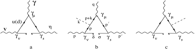
FIG. 3.: Operators of dimension 5 corrections proportional to $<\overline{q}\sigma\cdot Gq>$. The dot lines denote gluons.

FIG. 4.: The coupling constant g_ρηγ as a function of the Borel parameter $M^{2}$ for different values of ${M^{\prime}}^{2}$.

FIG. 5.: The coupling constant g_ωηγ as a function of the Borel parameter $M^{2}$ for different values of ${M^{\prime}}^{2}$.

REFERENCES

- [1] M. A. Shifman, A. I. Vainstein, V. I. Zakharov, Nucl. Phys. B 147 (1979) 385 and 448.
- [2] L. J. Reinders, S. Yazaki and H. R. Rubinstein, Nucl. Phys. B 196 (1985) 125.
- [3] B.L. Ioffe, Nucl. Phys. B 188 (1981) 317; B 191(1981) 591.
- [4] A.Gokalp, O.Yilmaz, Eur. Phys. J. C 24, (2002) 117
- [5] P. J. O’Donnell, Rev. Mod. Phys. 53 (1981) 673
- [6] P. Colangelo, A. Khodjamirian, in Boris Ioffe Festschrift, At the Frontier of Particle Physics / Handbook of the QCD, edited by M. Shifman World Scientific, Singapor.
- [7] [6] T.M.Aliev, I.Kanik, A.Ozpineci, hep-ph/0212187
- [8] A. V. Smilga, Sov. J. Nucl. Phys. 35 (1982) 271.
- [9] A. I. Titov, T. -S. H. Lee, H. Toki, O. Streltsova, Phys. Rev. C 60 (1999) 035205.
- [10] D. E. Groom et al., Eur. Phys. J. C15 (2000) 1;
- [11] S-L. Zhu, W-Y. P. Hwang, Z-S. Yang, Phys. Lett.B 420 (1998) 8.
- [12] V. L. Eletsky, B. L. Ioffe, Ya. I. Kogan, Phys. Lett.B 122 (1983) 423.