hep-ph/0303236

Variations of Little Higgs Models and their

Electroweak Constraints

Csaba Csáki^a, Jay Hubisz^a, Graham D. Kribs^b,

Patrick Meade^a, and John Terning^c

^a Newman Laboratory of Elementary Particle Physics,
Cornell University, Ithaca, NY 14853

^b Department of Physics, University of Wisconsin, Madison, WI 53706

^c Theory Division T-8, Los Alamos National Laboratory, Los Alamos, NM 87545

csaki@mail.lns.cornell.edu, hubisz@mail.lns.cornell.edu, kribs@physics.wisc.edu, meade@mail.lns.cornell.edu, terning@lanl.gov

We calculate the tree-level electroweak precision constraints on a wide class of little Higgs models including: variations of the Littlest Higgs $SU(5)/SO(5)$, $SU(6)/Sp(6)$, and $SU(4)^{4}/SU(3)^{4}$. By performing a global fit to the precision data we find that for generic regions of the parameter space the bound on the symmetry breaking scale $f$ is several TeV, where we have kept the normalization of $f$ constant in the different models. For example, the “minimal” implementation of $SU(6)/Sp(6)$ is bounded by $f>3.0$ TeV throughout most of the parameter space, and $SU(4)^{4}/SU(3)^{4}$ is bounded by $f^{2}\equiv f_{1}^{2}+f_{2}^{2}>(4.2\;\mathrm{TeV})^{2}$. In certain models, such as $SU(4)^{4}/SU(3)^{4}$, a large $f$ does not directly imply a large amount of fine tuning since the heavy fermion masses that contribute to the Higgs mass can be lowered below $f$ for a carefully chosen set of parameters. We also find that for certain models (or variations) there exist regions of parameter space in which the bound on $f$ can be lowered into the range $1$-$2$ TeV. These regions are typically characterized by a small mixing between heavy and standard model gauge bosons, and a small (or vanishing) coupling between heavy $U(1)$ gauge bosons and the light fermions. Whether such a region of parameter space is natural or not is ultimately contingent on the UV completion.

1 Introduction

Hierarchies in masses are ubiquitous in the Standard Model (SM). Fortunately, symmetries prevent gauge bosons and matter fermions from acquiring radiative corrections to their masses beyond logarithmic sensitivity to heavy physics. The Higgs boson mass, however, is quadratically sensitive to heavy physics. Hence, naturalness suggests the cutoff scale of the SM should be only a loop factor higher than the Higgs mass. However, there are many probes of physics beyond the SM at scales ranging from a few to tens of TeV. In particular, four-fermion operators that give rise to new electroweak (EW) contributions generally constrain the new physics scale to be more than a few TeV, and some new flavor-changing four-fermion operators are constrained even further, to be above the tens of TeV level. With mounting evidence for the existence of a light Higgs $\mathrel{\>{\hbox{\raise 1.50696pt\hbox{$<$}}\kern-3.8889pt\kern-3.8889pt\hbox{\lower 2.79857pt\hbox{$\sim$}}}\>}200$ GeV [1], we are faced with understanding why the Higgs mass is so light compared with radiative corrections from cutoff-scale physics that appears to have been experimentally forced to be above the tens of TeV level. The simplest solution to this “little hierarchy problem” is to fine-tune the bare mass against the radiative corrections, but is widely seen as being unnatural.

There has recently been much interest [2-15] in a new approach to solving the little hierarchy problem, called little Higgs models. These models have a larger gauge group structure appearing near the TeV scale into which the EW gauge group is embedded. The novel feature of little Higgs models is that there are approximate global symmetries that protect the Higgs mass from acquiring one-loop quadratic sensitivity to the cutoff. This happens because the approximate global symmetries ensure that the Higgs can acquire mass only through “collective breaking”, or multiple interactions. In the limit that any single coupling goes to zero, the Higgs becomes an exact (massless) Goldstone boson. Quadratically divergent contributions are therefore postponed to two-loop order, thereby relaxing the tension between a light Higgs mass and a cutoff of order tens of TeV.

The minimal ingredients of little Higgs models appear to be additional gauge bosons, vector-like colored fermions, and additional Higgs doublets and/or Higgs triplets, as well as scalars uncharged under the SM gauge group. In general modifications of the EW sector are usually tightly constrained by precision EW data (see Refs. [16-19] for example). One generic feature, new heavy gauge bosons, can be problematic if the SM gauge bosons mix with them or if the SM fermions couple to them. This is easy to see: Consider the modification to the coupling of a $Z$ to two fermions and (separately) the modification to the vacuum polarization of the $W$, as shown in Fig. 1. These are among the best measured EW parameters that agree very well with the SM predictions (using $M_{Z}$, $G_{F}$, and $\alpha_{em}$ as inputs): both of these observables have been measured to $\pm 0.2\%$ to 95% C.L. Generically the corrections to these observables due to heavy $U(1)$ gauge bosons and heavy $SU(2)$ gauge bosons can be simply read off from Fig. 1 as

$$\frac{\delta\Gamma_{Z}}{\Gamma_{Z}}\sim 1+c_{1}\frac{v^{2}}{f^{2}}\quad,\quad\frac{\delta M_{W}^{2}}{M_{W}^{2}}\sim 1+c_{2}\frac{v^{2}}{f^{2}}\;,$$ (1.1)

where $f$ is roughly the mass of the heavy gauge boson, and $c_{1}$ and $c_{2}$ parameterize the strength of the couplings between heavy-to-light fields. For $c_{1}\sim 1$ or $c_{2}\sim 1$, it is trivial to calculate the EW bound on $f$,

$$f>5.5\;\mbox{TeV}\quad\mbox{to 95\% C.L.}\;.$$ (1.2)

Notice that even if the coupling of light fermions to the heavy gauge bosons were zero ($c_{1}=0$), maximal mixing among $SU(2)$ gauge bosons ($c_{2}=1$) is sufficient to place a strong constraint on the scale of new physics.

Figure 1: Corrections to $\Gamma_{Z}$ and to $M_{W}^{2}$ through mixing with heavy gauge bosons.

In our previous paper [10] we examined the tree-level precision EW constraints on the Littlest Higgs model, $SU(5)/SO(5)$. We found strong constraints on the symmetry breaking scale $f$ consistent with the above naive argument. The reason for the appearance of these large corrections is that some interactions involving the heavy gauge bosons violate custodial $SU(2)$. However, the custodial $SU(2)$ violating corrections come mostly from the exchange of the heavy $U(1)$ gauge boson, thus one might try to adjust the $U(1)$ sector of the theory so that the contributions to the EW precision observables can be reduced. We examine such possibilities for the modifications of the $U(1)$ sector in the Littlest Higgs model in the first part of the paper, by including other $U(1)$ fermion charge assignments, gauging only $U(1)_{Y}$, and gauging a different combination of $U(1)$’s. In the second part of the paper we consider changing the global symmetry structure slightly (to the $SU(6)/Sp(6)$ model) and more drastically (the $SU(4)^{4}/SU(3)^{4}$ “simple group” model). Generically, meaning no special choices of the model parameters, we find that these models have constraints comparable to the those on the Littlest Higgs model. Unlike our previous analysis, however, we find regions of parameter space for certain models (or their variations) in which the bound on the symmetry breaking scale $f$ is lowered to $1$-$2$ TeV. We identify the extent of these regions of parameter space. Most recently a model based on $SO(5)^{8}/SO(5)^{4}$ which has a custodial $SU(2)$ has been proposed [9]. This model was specifically constructed to avoid constraints on the model from custodial $SU(2)$ violation from heavy gauge boson exchange. However, this model does contain $SU(2)$ triplets that could in principle lead to constraints, a complete analysis will be given in [20].

The organization of this paper is as follows. In Section 2 we review the Littlest Higgs model and consider the various possible $U(1)$ charge assignments. In Section 3 we examine what happens when different choices are made for the $U(1)$ gauge structure, including the case that the only gauged $U(1)$ is the standard hypercharge. In Section 4 we study the $SU(6)/Sp(6)$ model which has two Higgs doublets but no Higgs triplet. In Section 5 we consider the $SU(4)^{4}/SU(3)^{4}$ model. Finally, in Section 6 we conclude and discuss the implications of our results.

2 The Littlest Higgs: varying the U(1) embedding of the SM fermions

In the Littlest Higgs model, large contributions to EW precision observables arise from the exchange of the heavy $U(1)$ gauge boson [10, 11]. These large corrections are due to the custodial $SU(2)$ violating effects of the broken gauge sectors. Custodial $SU(2)$ violations form the heavy $SU(2)$ sector appear only at order $v^{4}/f^{4}$, which is negligible compared to the leading corrections of order $v^{2}/f^{2}$. These leading corrections arise from the exchange of the heavy $U(1)$ gauge boson, thus the $U(1)$ sector of the theory is the most problematic to EW precision constraints. The first modification we consider is to change the $U(1)\times U(1)$ charge assignments of the SM fermions. This has the potential to relax the bounds from EW precision observables by reducing the effective coupling to the heavy $U(1)$ gauge boson. In this section we examine this possibility after briefly reviewing the structure of the Littlest Higgs model.

2.1 The Littlest Higgs model

The Littlest Higgs model is based on the non-linear $\sigma$ model describing an $SU(5)/SO(5)$ global symmetry breaking [5]. This symmetry breaking can be thought of as originating from a VEV of a symmetric tensor of the $SU(5)$ global symmetry. A convenient basis for this breaking is characterized by the direction $\Sigma_{0}$ given by

$$\Sigma_{0}=\left(\begin{array}[]{ccccc}&&&1&\\ &&&&1\\ &&1\\ 1\\ &1\end{array}\right).$$ (2.1)

The Goldstone fluctuations are then described by the pion fields $\Pi=\pi^{a}X^{a}$, where the $X^{a}$ are the broken generators of $SU(5)$. The non-linear sigma model field is then

$$\Sigma(x)=e^{i\Pi/f}\Sigma_{0}e^{i\Pi^{T}/f}=e^{2i\Pi/f}\Sigma_{0}.$$ (2.2)

where $f$ is the scale of the VEV that accomplishes the breaking. An $[SU(2)\times U(1)]^{2}$ subgroup of the $SU(5)$ global symmetry is gauged, where the generators of the gauged symmetries are given by

$$Q_{1}^{a}=\left(\begin{array}[]{ccc}\sigma^{a}/2&0&0\\ 0&0&0\\ 0&0&0\end{array}\right),\ \ \ Y_{1}={\rm diag}(-3,-3,2,2,2)/10$$ (2.6)

$$Q_{2}^{a}=\left(\begin{array}[]{ccc}0&0&0\\ 0&0&0\\ 0&0&-\sigma^{a*}/2\end{array}\right), Y_{2}={\rm diag}(-2,-2,-2,3,3)/10~{},$$ (2.10)

where $\sigma^{a}$ are the Pauli $\sigma$ matrices. The $Q^{a}$’s are $5\times 5$ matrices written in terms of $2\times 2$, 1, and $2\times 2$ blocks. The Goldstone boson matrix $\Pi$, in terms of the uneaten fields, is then given by

$$\Pi=\left(\begin{array}[]{ccc}0&\frac{H^{\dagger}}{\sqrt{2}}&\phi^{\dagger}\\ \frac{H}{\sqrt{2}}&0&\frac{H^{*}}{\sqrt{2}}\\ \phi&\frac{H^{T}}{\sqrt{2}}&0\end{array}\right),$$ (2.11)

where $H$ is the little Higgs doublet $(h^{0},h^{+})$ and $\phi$ is a complex triplet Higgs, forming a symmetric tensor $\phi_{ij}$.

The kinetic energy term of the non-linear $\sigma$ model is

$$\frac{f^{2}}{8}{\rm Tr}D_{\mu}\Sigma(D^{\mu}\Sigma)^{\dagger}$$ (2.12)

where

$$D_{\mu}\Sigma=\partial_{\mu}\Sigma-i\sum_{j}\left[g_{j}W_{j}^{a}(Q_{j}^{a}\Sigma+\Sigma Q_{j}^{aT})+g_{j}^{\prime}B_{j}(Y_{j}\Sigma+\Sigma Y_{j})\right]~{},$$ (2.13)

and $g_{j}$ and $g_{j}^{\prime}$ are the couplings of $[SU(2)\times U(1)]_{j}$ gauge groups.

This structure of the gauge sector prevents quadratic divergences arising from gauge loops. In order to cancel the divergences due to the top quark the top Yukawa coupling is obtained from the operator

$${\cal L}_{top}=\frac{1}{2}\lambda_{1}f\epsilon_{ijk}\epsilon_{xy}\chi_{i}\Sigma_{jx}\Sigma_{ky}u_{3}^{\prime c}+\lambda_{2}f\tilde{t}\tilde{t}^{c}+\mbox{h.c.},$$ (2.14)

where $\chi=(b_{3}\;t_{3}\;\tilde{t})$, that preserves enough of the global symmetry to forbid a one-loop quadratic divergence arising from the top quark. The potential that gives rise to the Higgs quartic scalar interaction comes from the quadratically divergent terms in the Coleman-Weinberg (CW) potential and their tree level counterterms. Evaluating the contributions from both the gauge and fermion sector we find that the gauge loops contribute

$$af^{2}\left[(g_{2}^{2}+g_{2}^{\prime 2})\left|\phi_{ij}+\frac{i}{4f}(h_{i}h_{j}+h_{j}h_{i})\right|^{2}+(g_{1}^{2}+g_{1}^{\prime 2})\left|\phi_{ij}-\frac{i}{4f}(h_{i}h_{j}+h_{j}h_{i})\right|^{2}\right],$$ (2.15)

where $a$ is an order one constant determined by the relative size of the tree-level and loop-induced terms. Similarly, the fermion loops contribute

$$-a^{\prime}\lambda_{1}^{2}f^{2}\left|\phi_{ij}+\frac{i}{4f}(h_{i}h_{j}+h_{j}h_{i})\right|^{2},$$ (2.16)

where $\lambda_{1}$ (and $\lambda_{2}$) are the Yukawa couplings and mass terms. The $SU(3)$ global symmetries enforce the two possible combinations of $h$ and $\phi$ in the potential given above. Therefore two parameters $a$ and $a^{\prime}$ are sufficient to completely parameterize the potential.

2.2 Fermion U(1) charges

The $U(1)$ charges of the SM fermions are constrained by requiring that the Yukawa couplings are gauge invariant and maintaining the usual SM hypercharge assignment. The latter imposes the constraint $y_{1}+y_{2}=Y_{SM}$. For the top quark, the Yukawa coupling is fixed by the global symmetries (2.14), and hence its $U(1)$ charges are fixed. Furthermore, if mixed SM gauge group/$U(1)_{i}$ anomalies are to be avoided, the entire third generation $U(1)$ charges can be determined. We find that the $U(1)\times U(1)$ charges of the third generation are $Q:(\frac{1}{10},\frac{1}{15})$, $u_{3}:(-\frac{2}{5},-\frac{4}{15})$. The Yukawa couplings for the first and second generations and the down and lepton sectors can be written identically as in (2.14) with only the change of $\Sigma\to\Sigma^{*}$ in the down and lepton sectors and an extra fermion introduced for all the SM particles to cancel the one loop quadratic divergences. The charge assignments are determined just as they are for the third generation.

However, the quadratic divergences for the first two generations are much smaller than that of the top quark due to the small size of their Yukawa couplings. One could therefore ignore these numerically irrelevant quadratic divergences. This means the Yukawa couplings of the first two generations of fermions do not need to respect the global symmetries, and thus need not be of the form (2.14). Hence, the $U(1)$ charges of these fields could be modified [21].

Here we consider modifying the $U(1)$ charges of the first two generations to be different from the third generation. The same constraints enter as before, namely that the Yukawa couplings are gauge invariant and each light fermion retains its usual SM hypercharge as it must. The charges of a light fermion $F$ can be written as $RY_{F}$ under the first $U(1)$ and $(1-R)Y_{F}$ under the second $U(1)$, where $Y_{F}$ is the SM hypercharge of the fermion. We will also assume that $R$ is universal within each generation of fermions. This is the simplest assignment that avoids mixed SM gauge group/$U(1)_{i}$ anomalies. Also, we do not consider a different $R$ between the first two generations since this would lead to new contributions to flavor changing neutral current processes.

The possible values of $R$ can be determined by requiring the invariance of the Yukawa couplings under the $U(1)$’s. Given our assumptions above, it is sufficient to consider one light fermion Yukawa coupling, such as for up-type quarks

$$qhX^{r}Y^{s}u^{c}$$ (2.17)

where $X$ and $Y$ are the components of the $\Sigma$ field that get VEVs of order $f$, while $r$ and $s$ are assumed to be integers. Here, the field $X$ corresponds to the $(1,4)$ and $(2,5)$ components of the $\Sigma$ field and $Y$ corresponds to the $(3,3)$ component. The $U(1)$ charges of $X$ are $(\frac{1}{10},-\frac{1}{10})$ and for $Y$ they are $(\frac{4}{10},-\frac{4}{10})$. The $U(1)$ charges of the Higgs can be read off from its embedding into $\Sigma$ as either $(\frac{4}{10},\frac{1}{10})$ or $(\frac{1}{10},\frac{4}{10})$. (The two possibilities for the Higgs charge assignment are present because the light Higgs is a mixture of two fields with different $U(1)\times U(1)$ charge after the two $U(1)$’s are broken to the diagonal subgroup.) Assuming the Higgs field in (2.17) has the $U(1)$ charges $(\frac{4}{10},\frac{1}{10})$ (as would be the case for an operator of the type (2.14) with additional powers of $X$ and $Y$), we find that

$$R=(4-r+4s)/5,$$ (2.18)

i.e., $R$ can only take on integer multiples of $1/5$. Similarly, an operator involving the Higgs field with the other $U(1)\times U(1)$ charge assignment gives

$$R=(1-r+4s)/5.$$ (2.19)

In either case, only integer multiples of $1/5$ for $R$ are allowed. For the third generation, the top Yukawa coupling (2.14) corresponds to (2.17) with $r=1$ and $s=0$, and thus $R=3/5$. Therefore $R=3/5$ is the only value of $R$ whereby quadratic divergences can be canceled for fermions of every generation. Nevertheless we stress that this result is a consequence of our assumption that the modification of the $U(1)$ charges is universal within a generation. (If we drop this requirement there will be no simple constraints on the values of $R$.)

In [10] we calculated the tree-level EW precision constraints on the Littlest Higgs model assuming that the first two generation of fermions transformed only under the first gauge group, hence $R=1$. For this choice of light fermion $U(1)$ charges we found the bound on $f$ to be 4 TeV with a fine-tuning in the Higgs mass of less than a percent. We now redo our calculations for the corrections to EW precision observables for generic values of $R$. As we explained in [10], the main quantities that are necessary to compute the EW precision observables are: the $W$ and $Z$ masses $M_{W}$ and $M_{Z}$, the Fermi coupling $G_{F}$, the shifts in the couplings of the $Z$ boson to the light fermions $\delta\tilde{g}^{FF}$, and the low-energy neutral current Lagrangian parameterized in terms of $\rho_{*}$ and $s_{*}^{2}(0)$. The detailed definition of these quantities, as well as the observed and bare values of the weak mixing angle $s_{0}^{2}$ and $s_{W}^{2}$ is given in [10,22-26]. We find the above quantities re-expressed as a function of $R$ to be:

$$M_{W}^{2} = \frac{g^{2}v^{2}}{4}\left(1+\frac{\Delta}{4}(1+4c^{2}-4c^{4})+4\Delta^{\prime}\right)$$

$$M_{Z}^{2} = \frac{(g^{2}+g^{\prime 2})v^{2}}{4}\left(1+\frac{\Delta}{4}(1+4c^{2}-4c^{4})-\frac{5\Delta}{4}(1-2c^{\prime 2})^{2}+8\Delta^{\prime}\right)$$

$$\delta\tilde{g}^{FF} = \Delta/2\left[(5(c^{\prime 2}s^{\prime 2}+c^{\prime 4}(R-1)-s^{\prime 4}R)+c^{2}(1-2c^{2}))T_{3}^{F}\right.$$

$$\,\,\,\,\,\,\,\,\,\,\,\,\,\,\,\,\left.-5(c^{\prime 2}s^{\prime 2}+c^{\prime 4}(R-1)-s^{\prime 4}R)Q_{F}\right]$$

$$\rho_{*} = 1-4\Delta^{\prime}+\frac{5}{4}\Delta(1-2R)^{2}$$

$$s_{*}^{2}(0) = s_{W}^{2}+\frac{\Delta}{2}\left[5R(s_{W}^{2}-1)(1-2R)+5c^{\prime 2}(s_{W}^{2}-1)(2R-1)-c^{2}s_{W}^{2}\right]$$

$$s_{0}^{2} = s_{W}^{2}-\frac{s_{W}^{2}c_{W}^{2}}{c_{W}^{2}-s_{W}^{2}}\left[\Delta\left(c^{2}-c^{4}-\frac{5}{4}(1-2c^{\prime 2})^{2}\right)+4\Delta^{\prime}\right]$$

$$G_{F} = \frac{1}{\sqrt{2}v^{2}}\left(1-\frac{\Delta}{4}-4\Delta^{\prime}\right)~{}.$$ (2.20)

where we have defined (as in [10])

$$\Delta=\frac{v^{2}}{f^{2}};\;\;\Delta^{\prime}=\frac{v^{\prime 2}}{v^{2}};\;\;c=\frac{g}{g_{2}};\;\;c^{\prime}=\frac{g^{\prime}}{g_{2}^{\prime}},$$ (2.21)

and $v^{\prime}$ is the VEV of the scalar $SU(2)$ triplet. Using these expressions all the EW precision observables can be obtained as in [10].

The largest contribution to the constant shift in the observables listed in the Appendix of [10] comes from the $U(1)$ sector of the theory (plus the constant shift coming from the triplet VEV). In the following section we calculate the bounds on $f$ for a general $R$. The light fermion coupling to the heavy $B$ vanishes for $R=1/2$ and $c^{\prime}=1/\sqrt{2}$. The decoupling of the corrections resulting from exchange of the heavy $B$ gauge boson is evident in the above expressions for which all corrections to the EW observables coming from the $U(1)$ sector of the theory disappear in this limit. However some corrections, such as $\rho_{*}$ vanish (not including those coming from the triplet VEV) in only the $R=1/2$ limit and are angle independent. However, $R=1/2$ is inconsistent with the gauge invariance of our Yukawa coupling (2.17), and so these corrections can never disappear simply from judicious choices of the $U(1)$ charges. However, since the triplet VEV corrections go in the opposite direction of the $U(1)$ corrections it is not necessary to have $R=1/2$ exactly.

2.3 Numerical bounds

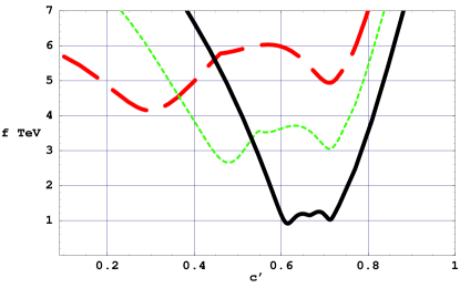
Figure 2: The 95% confidence level bound is shown for $a=1$ and $R=1$ (dashed), $R=4/5$ (dotted), and $R=3/5$ (solid). The bounds for $R=2/5,1/5$ and $0$ can be obtained by reflecting the above curves around $c^{\prime 2}=1/2$ due to the $R\to 1-R$, $c^{\prime 2}\to 1-c^{\prime 2}$ symmetry of the expressions for the EW corrections.

To analyze the bounds on the model we have performed a three-parameter fit ($f,c,c^{\prime}$) for the allowed values of $R=1,4/5,3/5,2/5,1/5$ and $0$. This determines the gauge sector of the model, but there is also the additional parameter $a$ in the Coleman-Weinberg potential of the Littlest Higgs that affects the size of the triplet VEV. The parameter $a$ is expected to be ${\cal O}(1)$; we consider fixed values of $a$ in the range $0.5$-$5$. To ensure the high energy gauge couplings $g_{1,2},g^{\prime}_{1,2}$ are not too strongly coupled, the angles $c,s,c^{\prime},s^{\prime}$ cannot be too small. As before [10] we allow for $c,s,c^{\prime},s^{\prime}>0.1$, or equivalently $0.1<c,c^{\prime}<0.995$. We allow $f$ to take on any value (although for small enough $f$ there will be constraints from direct production of $B_{H}$). The general procedure we used is to systematically step through values of $c$ and $c^{\prime}$, finding the lowest value of $f$ that leads to a shift in the $\chi^{2}$ corresponding to the 95% confidence level (C.L.). For a three-parameter fit, this corresponds to a $\Delta\chi^{2}$ of about $7.8$ from the minimum. In Fig. 2 the allowed values of $f$ are plotted as a function of $c$ for fixed values of $R$ and $a$ and one sees that the value of allowed $f$ dips down to $1\,\mbox{TeV}$ for $R=3/5$.

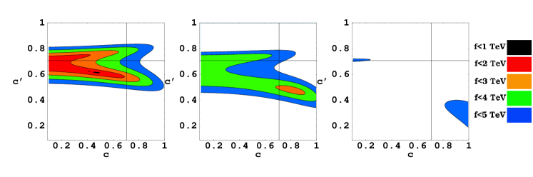
Figure 3: Contours of the minimum allowed values of $f$ at 95% C.L. for $a=1$ and $R=3/5$ (left graph) $R=4/5$ (center graph) $R=1$ (right graph).

In Fig. 2 the value of $c$ has already been chosen to minimize the bound on $f$ so this only shows the size of allowed parameter space in $c^{\prime}$. In Fig. 3 we plot for fixed $R=3/5,4/5,1$ and $a=1$ a contour plot showing the allowed range of parameter space at 95% C.L. for both $c$ and $c^{\prime}$ showing the size of the allowed region of parameter space for a given value of $R$ and $a$. We see in Fig. 3 that the allowed region where the bound on $f$ reaches $1$ TeV is extremely small. So, the Littlest Higgs with $R=3/5$ does have regions of parameter space where the bound on $f$ is around $2$ TeV and thus the fine-tuning in the Higgs mass is minimized. Nevertheless, the size of this region is not particularly large for $f\leq 2$ TeV, and for $f\leq 1$ TeV it is essentially just a point in parameter space.

Next, we consider how varying the value of $a$ affects the minimum value of $f$ and the size of the allowed parameter regions at 95% C.L. Since the parameter $a$ not only affects the size of the VEV but also feeds into the triplet mass, there is an additional constraint on $a$ upon requiring a positive triplet (mass)². If the triplet (mass)² were negative the triplet would obtain a VEV of order $f$ that would introduce zeroth order corrections to precision EW observables, and is thus ruled out. Following the same procedure as outlined above, we recalculate the bounds varying $a$ discretely between $a=0.5$ to $a=5$ and show the allowed regions at 95% C.L. in Fig. 4. The additional shaded areas are those excluded by ensuring the triplet (mass)² is positive.

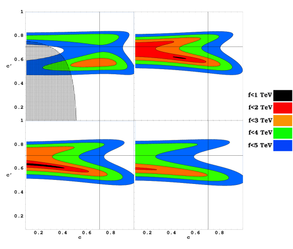
Figure 4: Plot of allowed values of $f$ at $95$ % C.L. for $a=0.5,1,2,5$ starting from the upper left corner in respective clockwise order, and fixed $R=3/5$. The shaded grey region corresponds to the parameter space excluded due to a negative triplet (mass)². We do not show $a=0.1$ since virtually the entire region is excluded due to a negative triplet (mass)².

Fig. 4 shows that perturbing $a$ from one generally reduces the allowed region of parameter space for a given $f$. For small values of $a$ the exclusion region due to requiring a positive triplet (mass)² is large.

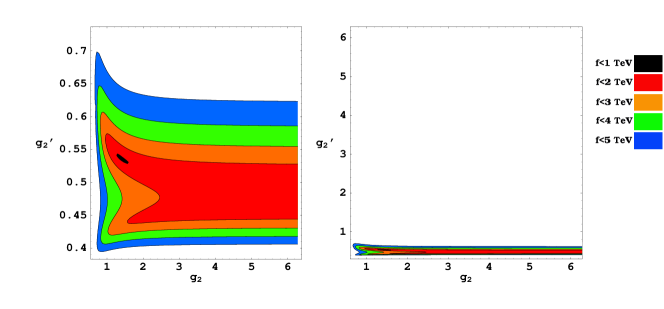
Figure 5: The plot on the left corresponds to the phenomenologically viable region of parameter space in $g_{2}$ and $g_{2}^{\prime}$ between $0$ and $2\pi$ with allowed values of $f$ at 95% C.L.. The plot on the right corresponds to showing all possible values of $g_{2}$ and $g_{2}^{\prime}$ between $0$ and $2\pi$ with allowed values of $f$ at 95% C.L.

In Fig. 5 we demonstrate the allowed region of parameter space in the actual couplings $g_{2}$ and $g_{2}^{\prime}$. Due to the non-linear mapping between the angles and the physical couplings we see that the allowed region in the physical coupling space is quite small. Similarly, plotting in the space of $g_{1}$ and $g_{1}^{\prime}$ one finds the allowed regions are even smaller. Plotting the physical couplings illustrates that the small but finite extent of the allowed region in $c$ and $c^{\prime}$ space is even further suppressed in the physical coupling space.

To demonstrate the significance of the bounds on $f$ we quantify the amount of fine tuning necessary as done in [5]. The heavy fermion (with mass $m^{\prime}$) introduced to cancel the top loop divergence of the SM contributes

$$-\frac{3\lambda_{t}^{2}}{4\pi^{2}}m^{\prime 2}\log\frac{4\pi f}{m^{\prime}}$$ (2.22)

to the Higgs mass squared. Given the bound on the mass of the heavy fermion $m^{\prime}>\sqrt{2}f$ as calculated in [10] we can calculate the percentage of fine-tuning required for a given value of $f$. In Fig. 3 the contours are plotted for the regions $f<(1,2,3,4,5)$ TeV and $f>5$ TeV, this corresponds to a fine tuning (assuming a physical Higgs mass of order 200 GeV) of more than $(14.3,3.6,1.6,0.9,0.6)\%$ and less than $0.6\%$ respectively. One can see from Fig. 3 that there are regions in parameter space where the fine-tuning is on the order of 10% but they are very small.

3 Modifying the Littlest Higgs

In the Littlest Higgs model, the largest contributions to the EW precision observables come from the $U(1)$ sector. We have already seen that modifying the light fermion charges is one alternative that can relax the bounds on the model. Here we examine two possibilities for modifying the $U(1)$ sector: choosing $U(1)$’s that are not necessarily subgroups of the global $SU(5)$; and, gauging only $U(1)_{Y}$ [21]. We will examine the benefits and drawbacks of each of these two possibilities.

3.1 Changing the gauged U(1)’s

If we do not insist that the gauged $U(1)$’s be $SU(5)$ subgroups then we can introduce a new parameter $b$ with which the $U(1)$’s are modified to

$$Y_{1}=\mbox{diag}\,(-3,-3,2,2,2)/10+bI,$$ (3.1)

$$Y_{2}=\mbox{diag}\,(-2,-2,-2,3,3)/10-bI,$$ (3.2)

where $I$ is the $5$ by $5$ unit matrix. This modification of the $U(1)$ sector does not change the $U(1)_{Y}$ quantum numbers and can be effectively thought of as a way to decouple the heavy $U(1)$ gauge bosons. This introduces an extra singlet into the Goldstone boson matrix, whose effects we ignore. One can easily see that that for the cases $b=1/5$ or $b=-1/5$ that the $U(1)$’s are orthogonal. This would be a preferred value of $b$, since then the issue of loop induced kinetic mixing terms would not arise. When computing the bare expressions in this modified model we find for instance that

$$\rho_{*}=1+\frac{5}{4}(1-2R)^{2}\Delta\left(\frac{1}{1+100b^{2}}\right)-4\Delta^{\prime}$$ (3.3)

compared with

$$\rho_{*}=1+\frac{5}{4}(1-2R)^{2}\Delta-4\Delta^{\prime}$$ (3.4)

in the Littlest Higgs model. Here $R$ is again characterizing the embedding of the fermions into $U(1)_{1}\times U(1)_{2}$ as in the previous section. The $1/(1+100b^{2})$ factor suppresses all other $U(1)$ dependent expressions as well and thus naively would be thought of as a very efficient way to get rid of the bound on $f$. The reason is that for large values of $b$ the heavy $U(1)$ gauge boson would live mostly in the $U(1)$ which is not part of $SU(5)$ (the extra $U(1)$ of $U(5)$) which does not violate custodial $SU(2)$. The effect of the new $U(1)$ on other quantities is similar and is as follows:

$$M_{W}^{2} = \frac{g^{2}v^{2}}{4}\left(1+\frac{\Delta}{4}(1+4c^{2}-4c^{4})+4\Delta^{\prime}\right)$$ (3.5)

$$M_{Z}^{2} = \frac{(g^{2}+g^{\prime 2})v^{2}}{4}\left(1+\frac{\Delta}{4}(1+4c^{2}-4c^{4})-\frac{\Delta 5(1-2c^{\prime 2})^{2}}{4(1+100b^{2})}+8\Delta^{\prime}\right)$$ (3.6)

$$s_{*}^{2}(0) = s_{W}^{2}+\frac{\Delta}{2}\left(-c^{2}s_{W}^{2}+\frac{5c_{W}^{2}}{1+100b^{2}}(-1+c^{\prime 2}+R)(2R-1)\right)$$ (3.7)

$$s_{0}^{2} = s_{W}^{2}-\frac{s_{W}^{2}c_{W}^{2}}{c_{W}^{2}-s_{W}^{2}}\left[\Delta\left(c^{2}-c^{4}-\frac{5}{4(1+100b^{2})}(1-2c^{\prime 2})^{2}\right)+4\Delta^{\prime}\right]$$ (3.8)

$$G_{F} = \frac{1}{\sqrt{2}v^{2}}\left(1-\frac{\Delta}{4}-4\Delta^{\prime}\right)$$ (3.9)

However, we need to make sure that the Yukawa couplings remain invariant under the modified $U(1)$ charge assignments. In order for the operator giving rise to the top Yukawa coupling in (2.14) to be invariant we need the relation

$$R=\frac{3+40b}{5}$$ (3.10)

to be satisfied. If we insist that all three families have the same charge assignments (that is that all the one loop quadratic divergences could be canceled at least in principle) then this relation needs to hold for the first two families as well. In order to get $b=\pm 1/5$ for orthogonal $U(1)$’s we must have $R=11/5$ and $R=-1$ respectively. For such large values of $R$ the corrections to EW observables would in fact increase, not decrease. For example one can see that the expression for $\rho_{*}$ does not go to 1 if we increase $b$, but rather asymptotes to $1+16/5\Delta$ for large $b$. Thus very large values of $b$ (contrary to our original expectation) will not be helpful. However, one can still use this freedom to slightly relax the bounds obtained in the previous section. The reason is that by picking $b=-\frac{1}{80}$ one can set $R=\frac{1}{2}$, in which case the heavy $U(1)$ gauge boson contributions to EW precision observables can almost all be eliminated, its coupling to the fermions can be eliminated. Previously this point was not allowed as long as we restricted ourselves to operators with integer powers of fields.

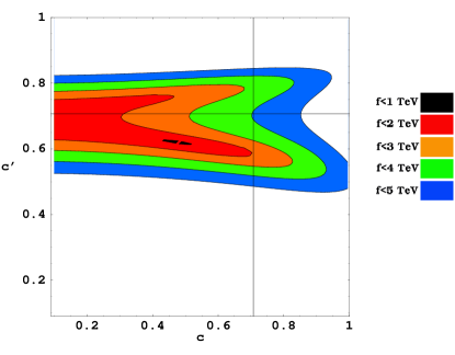
Figure 6: Contour plot of allowed values of $f$ as a function of the angles $c$ and $c^{\prime}$ for $R=1/2$ and $a=1$ and $b=-1/80$.

The region allowed at the 95% CL by the EW precision fit for the $R=1/2,b=-1/80$ case is shown in Fig. 6. We can see that the region corresponding to the smallest fine tuning ($f<2$ TeV) is slightly, but not significantly, larger than in the cases considered in the previous section, and there is now a non-negligible region where $f$ would be less than $1$ TeV.

3.2 Gauging only U(1)_Y

Since many of the corrections actually originate from the exchange of the heavy $U(1)$ gauge boson, one way to try to improve the EW precision bounds is by eliminating the heavy $U(1)$ and only gauging the SM $U(1)_{Y}$ subgroup [21]. This again leaves an extra scalar in the $\Pi$ matrix whose effects we ignore. In the case where only one $U(1)_{Y}$ is gauged all constant corrections in $\Delta$ and $U(1)$ angle dependent pieces in our bare expressions disappear. We calculate all the corrections from the kinetic term which is

$$\frac{f^{2}}{8}{\rm Tr}D_{\mu}\Sigma(D^{\mu}\Sigma)^{\dagger}$$ (3.11)

where now

$$D_{\mu}\Sigma=\partial_{\mu}\Sigma-i\sum_{j}\left[g_{j}W_{j}^{a}(Q_{j}^{a}\Sigma+\Sigma Q_{j}^{aT})\right]-ig^{\prime}B(Y_{SM}\Sigma+\Sigma Y_{SM})~{},$$ (3.12)

where $g_{j}$ is the coupling of the $[SU(2)]_{j}$ gauge group, and $g^{\prime}$ is the coupling of the $U(1)_{Y}$ gauge group. The generator for $U(1)_{Y}$ is $Y_{SM}=\mbox{diag}(-1/2,-1/2,0,1/2,1/2)$. Recalculating the relevant quantities for this case yields:

$$M_{W}^{2} = \frac{g^{2}v^{2}}{4}\left(1+\frac{\Delta}{4}(1+4c^{2}-4c^{4})+4\Delta^{\prime}\right)$$ (3.13)

$$M_{Z}^{2} = \frac{(g^{2}+g^{\prime 2})v^{2}}{4}\left(1+\frac{\Delta}{4}(1+4c^{2}-4c^{4})+8\Delta^{\prime}\right)$$ (3.14)

$$s_{*}^{2}(0) = s_{W}^{2}+\frac{\Delta}{2}\left(-c^{2}s_{W}^{2}\right)$$ (3.15)

$$s_{0}^{2} = s_{W}^{2}-\frac{s_{W}^{2}c_{W}^{2}}{c_{W}^{2}-s_{W}^{2}}\left[\Delta\left(c^{2}-c^{4}\right)+4\Delta^{\prime}\right]$$ (3.16)

$$G_{F} = \frac{1}{\sqrt{2}v^{2}}\left(1-\frac{\Delta}{4}-4\Delta^{\prime}\right)$$ (3.17)

$$\rho_{*} = 1-4\Delta^{\prime}$$ (3.18)

We see from these expressions we still retain our constant shifts in $\Delta^{\prime}$ to our bare observables. We must compute the scalar Higgs potential coming from the quadratically divergent pieces of the Coleman-Weinberg(CW) potential so as to estimate the size of the triplet VEV in this particular model. The quadratically divergent piece of the CW potential from the gauge bosons is

$$\frac{\Lambda^{2}}{16\pi^{2}}\mbox{Tr}M_{V}^{2}(\Sigma),$$ (3.19)

where $M_{V}^{2}$ is the gauge boson mass matrix in an arbitrary $\Sigma$ background. $M_{V}^{2}$ can be read off from the covariant derivative for $\Sigma$, giving a potential

$$ag_{j}^{2}f^{4}\sum_{a}\mbox{tr}\left[(Q_{j}^{a}\Sigma)(Q_{j}^{a}\Sigma)^{*}\right]+ag^{\prime}f^{4}\mbox{tr}\left[(Y_{SM}\Sigma)(Y_{SM}\Sigma)^{*}\right]$$ (3.20)

where $a$ is a constant of order one determined by the relative size of the tree-level and loop induced terms, and we have used $\Lambda\sim 4\pi f$. We also have a quadratically divergent contribution to the CW potential coming from the fermion loops. This potential from the fermion sector contributes the same potential as that generated from the $SU(2)_{2}$ gauge bosons since the operator that gives the fermion potential is $SU(3)_{1}$ symmetric. Calculating the VEV of $\phi$ we obtain

$$v^{\prime}=\frac{iv^{2}}{4f^{2}}\frac{a^{\prime}\lambda_{1}^{2}+a(g_{1}^{2}-g_{2}^{2})}{-a^{\prime}\lambda_{1}^{2}+a(4g^{\prime 2}+g_{1}^{2}+g_{2}^{2})}$$ (3.21)

where $a^{\prime}$ is an order one coefficient parameterizing the fermion operator that contributes to the CW potential and $\lambda_{1}$ is the Yukawa coupling of that operator. We can integrate out the triplet to generate a quartic coupling for the Higgs

$$\lambda=\frac{a(-a^{\prime}\lambda_{1}^{2}(2g^{\prime 2}+3g_{1}^{2})+a(-4g^{\prime 4}+3g_{1}^{2}g_{2}^{2}+2g^{\prime 2}(g_{1}^{2}+g_{2}^{2})))}{3(-a^{\prime}\lambda_{1}^{2}+a(4g^{\prime 2}+g_{1}^{2}+g_{2}^{2}))}.$$ (3.22)

and thus we obtain that

$$\Delta^{\prime}\equiv\frac{|v^{\prime}|^{2}}{v^{2}}=\frac{\Delta}{144}\left[1+\frac{6\lambda-4ag_{1}^{2}}{a(2g^{\prime 2}+g_{1}^{2})}\right]^{2}.$$ (3.23)

There is one further constraint that requires the triplet mass to be positive so the triplet does not obtain a VEV at the scale $f$. The positivity of the triplet mass requires

$$a(4g^{\prime 2}+g_{1}^{2}+g_{2}^{2})-a^{\prime}\lambda_{1}^{2}>0$$ (3.24)

which is equivalent to [using (3.22)]

$$2ag^{\prime 2}-3\lambda+3ag_{1}^{2}>0.$$ (3.25)

This constraint combined with (3.23) gives us that

$$\Delta^{\prime}<\frac{\Delta}{16}.$$ (3.26)

It is important to note that even though $\Delta^{\prime}$ is small, the coefficients of $\Delta^{\prime}$ in the contributions to observables are constant and can not be fully tuned away except in small regions of parameter space.

Using the bare expressions and re-expressing them in terms of observables we are able to calculate the bounds on the Littlest Higgs when we only gauge $U(1)_{Y}$.

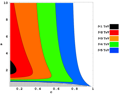
Figure 7: Contour plot of the allowed values of $f$ as a function of $a$ and $c$. The x-axis is $c$ and the y-axis is $a$. The grey shaded region at the bottom corresponds to the region excluded by requiring a positive triplet mass.

In Fig. 7 we have plotted the allowed values of $f$ as a function of $c$ which parameterizes the $SU(2)$ mixing and $a$ which parameterizes the strength of the gauge contribution to the CW potential. From Fig. 7 we see that in a relatively small region of parameter space the bounds on $f$ make the model acceptable from a fine tuning perspective using the measure of fine tuning defined as (2.22).

In the region of small $f$, the triplet vev contributions are negligible, and the $SU(2)$ corrections are small due to suppression by factors of $c$, thus one should ask how the inclusion of loop contributions from the additional particles to $T$ and $\rho_{*}(0)$ might affect the location and size of this region. The largest contribution is coming from the additional heavy vector-like top quarks. The leading contribution beyond what is induced by the normal SM loops is then given by

$$\Delta\rho_{\mathrm{top}}=\frac{N_{c}\Delta}{16\pi^{2}}\left(\frac{\lambda_{t}^{4}}{2\lambda_{H}^{2}}\right)\log\left[\frac{2\lambda_{H}^{2}}{\lambda_{t}^{2}\Delta}\right],$$ (3.27)

where $\lambda_{H}\equiv\sqrt{\lambda_{1}^{2}+\lambda_{2}^{2}}$, with $\lambda_{1}$ and $\lambda_{2}$ defined in (2.14). Note that $\lambda_{H}$ has a minimum value of $\lambda_{H}=\sqrt{2}$. One can see that this contribution decouples for $f\to\infty$, and is not important for establishing the bounds as long as the tree-level contributions are already forcing $f$ to be large. However, for the regions with small $f$ these contributions are comparable to the non-canceled pieces of the tree-level effect, and thus might be relevant when one is trying to find the precise shape of the allowed regions. (3.27) can be interpreted as a $T$ contribution for the $Z$-pole observables, and as a correction to $\rho_{*}(0)$ in the low energy observables. The results of including the maximal shift are shown in Fig. 8. Note that the regions where $f$ goes below $1$ TeV are slightly shifted above $1$ TeV.

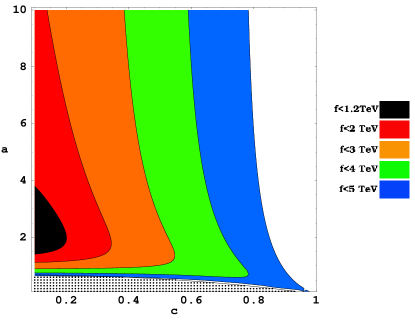
Figure 8: Shown above is a contour plot with only one $U(1)$ gauged in a variation on the Littlest Higgs model. We have chosen a different lowest contour because the region with the lowest $f$ is shifted slightly above $1$ TeV.

The drawback of this model is that without gauging a second $U(1)$ the one-loop quadratic divergences to the Higgs mass from $U(1)_{Y}$ do not cancel. Therefore in the case of gauging only $U(1)$ we will introduce divergences of the form

$$\frac{1}{16\pi^{2}}g^{\prime 2}\Lambda^{2}.$$ (3.28)

For $\Lambda\sim 10\,\mbox{TeV}$ this implies a fine tuning of the Higgs mass of approximately $50$ percent, which is obviously preferable to the level of fine tuning that the original little Higgs models generically had. However, in this case we are giving up on the concept of systematically eliminating all one-loop quadratic divergences arising from interactions with order one coefficients.

4 SU(6)/Sp(6) Little Higgs

To determine whether the bounds on $f$ are generically large in little Higgs coset models, here we consider the $SU(6)/Sp(6)$ model proposed in [7].

4.1 The SU(6)/Sp(6) model

This model is based on an anti-symmetric condensate breaking a global $SU(6)$ to $Sp(6)$ in contrast to the symmetric condensate breaking used in [5]. The basis for the breaking is characterized by the direction $\Sigma_{0}$ which is given by

$$\langle\Sigma_{0}\rangle=\left(\begin{array}[]{cc}0&-I\\ I&0\\ \end{array}\right),$$ (4.1)

where $I$ is the $3$ by $3$ unit matrix. The Goldstone bosons are then described by the pion fields $\Pi=\pi^{a}X^{a}$, where the $X^{a}$ are the broken generators of the $SU(6)$. The non-linear sigma model field is then

$$\Sigma=e^{i\Pi/f}\Sigma_{0}e^{i\Pi^{T}/f}=e^{2i\Pi/f}\Sigma_{0},$$ (4.2)

where $f$ is the scale of the VEV that accomplishes the breaking. An $SU(2)^{2}$ portion of the $SU(6)$ global symmetry is gauged, where the generators are

$$Q_{1}^{a}=\frac{1}{2}\left(\begin{array}[]{c|c}\begin{array}[]{c|c}\mbox{\Large$\sigma^{a}$}&0\\ \hline\cr 0&0\\ \end{array}&\;\;\;\mbox{\Large$0$}\\ \hline\cr&\\ \mbox{\Large$0$}&\;\;\;\mbox{\Large$0$}\\ &\\ \end{array}\right)\hskip 30.0pt{\rm and}\hskip 30.0ptQ_{2}^{a}=-{\frac{1}{2}}\left(\begin{array}[]{c|c}&\\ \mbox{\Large$0$}&\;\;\;\mbox{\Large$0$}\\ &\\ \hline\cr\;\;\;\mbox{\Large$0$}&\begin{array}[]{c|c}&\\ \mbox{\Large$\sigma^{a*}$}&0\\ \hline\cr 0&0\\ \end{array}\\ \end{array}\right),$$ (4.3)

where $\sigma^{a}$ are the Pauli $\sigma$ matrices. There are also two gauged $U(1)$’s that are not a subgroup of the global $SU(6)$ which are given by

$$Y_{1}=\mbox{diag}(0,0,-1/2,0,0,0)$$ (4.4)

and

$$Y_{2}=\mbox{diag}(0,0,0,0,0,1/2).$$ (4.5)

The Goldstone boson matrix $\Pi$ is expressed in terms of the uneaten fields as

$$\Pi=\left(\begin{array}[]{c|c|c|c}\mbox{\LARGE$0$}&\frac{\phi_{1}}{\sqrt{2}}&\begin{array}[]{cc}0&s\\ -s&0\\ \end{array}&\frac{\phi_{2}}{\sqrt{2}}\\ \hline\cr\phi_{1}^{\dagger}/\sqrt{2}&0&-\phi_{2}^{T}/\sqrt{2}&0\\ \hline\cr\begin{array}[]{cc}0&-s^{*}\\ s^{*}&0\\ \end{array}&-\frac{\phi_{2}^{*}}{\sqrt{2}}&\mbox{\LARGE$0$}&\frac{\phi_{1}^{*}}{\sqrt{2}}\\ \hline\cr\phi_{2}^{\dagger}/\sqrt{2}&0&\phi_{1}^{T}/\sqrt{2}&0\\ \end{array}\right).$$ (4.6)

In this model $\phi_{1}$ and $\phi_{2}$ transform under $SU(2)_{W}$ and $U(1)_{Y}$ as $\mathbf{2}_{1/2}$ and $\mathbf{2}_{-1/2}$ respectively, whereas $s$ transforms as $\mathbf{1}_{0}$. The kinetic term of the non-linear sigma model field is

$$-\frac{f^{2}}{8}\mbox{Tr}[(D_{\mu}\Sigma)(D^{\mu}\Sigma)^{*}]$$ (4.7)

where

$$D_{\mu}\Sigma=\partial_{\mu}\Sigma-\sum_{j}[ig_{j}W_{j}^{a}(Q_{j}^{a}\Sigma+\Sigma Q_{j}^{aT})+ig_{j}^{\prime}B_{j}(Y_{j}\Sigma+\Sigma Y_{j}^{T})]$$ (4.8)

where $g_{j}$ and $g_{j}^{\prime}$ are the couplings of $[SU(2)\times U(1)]_{j}$ gauge groups. Following the same procedure as in [10] we expand the kinetic term in $\Sigma$ to second-order. (In this model we have to expand to second order since we have two Higgs doublets and can not redefine just one VEV when expanding from linear to higher orders as could be done in the Littlest Higgs model.) The heavy gauge bosons acquire masses

$$M_{W_{H}} = \sqrt{g_{1}^{2}+g_{2}^{2}}\frac{f}{2}~{},$$ (4.9)

$$M_{B_{H}} = \sqrt{g_{1}^{\prime 2}+g_{2}^{\prime 2}}\frac{f}{2\sqrt{2}}~{}.$$ (4.10)

Note, that contrary to the Littlest Higgs model the heavy $U(1)$ gauge boson is not significantly lighter than the $SU(2)$ gauge bosons, which itself reduces the bounds slightly. The VEV’s the $\phi$’s acquire are

$$\langle\phi_{1}\rangle=\frac{1}{\sqrt{2}}\left(\begin{array}[]{c}0\\ v_{1}\\ \end{array}\right)\mbox{ and }\langle\phi_{2}\rangle=\frac{1}{\sqrt{2}}\left(\begin{array}[]{c}v_{2}\\ 0\\ \end{array}\right),$$ (4.11)

which we will redefine in terms of

$$v^{2}=v_{1}^{2}+v_{2}^{2}$$ (4.12)

and

$$\tan\beta=\frac{v_{2}}{v_{1}}.$$ (4.13)

The singlet which is very heavy will also get a VEV however it is neutral and does not enter into any of our expressions. We will also make further simplifications by defining

$$\Delta=v^{2}/f^{2},$$ (4.14)

$$s=\frac{g_{2}}{\sqrt{g_{1}^{2}+g_{2}^{2}}},c=\frac{g_{1}}{\sqrt{g_{1}^{2}+g_{2}^{2}}},s^{\prime}=\frac{g_{2}^{\prime}}{\sqrt{g_{1}^{\prime 2}+g_{2}^{\prime 2}}},c^{\prime}=\frac{g_{1}^{\prime}}{\sqrt{g_{1}^{\prime 2}+g_{2}^{\prime 2}}},$$ (4.15)

$$g=g_{1}s,g^{\prime}=g_{1}^{\prime}s^{\prime},\;\mbox{ and }s_{W}=\frac{g^{\prime}}{\sqrt{g^{2}+g^{\prime 2}}}$$ (4.16)

4.2 Contributions to electroweak observables

We assume all left-handed fermions are charged only under $SU(2)_{1}$. Analogous to our discussion in a variation of the Littlest Higgs model, we allow fermions to couple to both $U(1)$’s with a constant $R$ varying from $0$ to $1$ characterizing the coupling to $U(1)_{1}$ ($R=1$) and $U(1)_{2}$ ($R=0$). Below we will determine the restrictions on the parameter $R$ by requiring gauge invariance of the Yukawa couplings.

Expanding the relevant bare expressions to first order in $\Delta$ we find

$$M_{W}^{2} = g^{2}\frac{v^{2}}{4}\left(1-\frac{\Delta}{4}(1-4c^{2}+4c^{4}-\cos^{2}2\beta)\right)$$

$$M_{Z}^{2} = (g^{2}+g^{\prime 2})\frac{v^{2}}{4}\left(1-\frac{\Delta}{4}(1-4c^{2}+4c^{4}+2(s^{\prime 2}-c^{\prime 2})^{2})\right)$$

$$G_{F} = \frac{1}{\sqrt{2}v^{2}}\left(1+\frac{\Delta}{4}(1-\cos^{2}2\beta)\right)$$

$$\delta\tilde{g}_{ff} = T^{3}\frac{\Delta}{2}\left(-2+c^{2}-2\,c^{4}+6\,c^{\prime 2}-4\,c^{\prime 4}+2\,R-4\,c^{\prime 2}\,R\right)$$

$$+Q\Delta\left(-1+2\,c^{\prime 2}\right)\,\left(-1+c^{\prime 2}+R\right)$$

$$s_{0}^{2} = s_{W}^{2}+\frac{s_{W}^{2}c_{W}^{2}}{c_{W}^{2}-s_{W}^{2}}\frac{\Delta}{4}\left[2-4\,c^{2}+4\,c^{4}-8\,c^{\prime 2}+8\,c^{\prime 4}+\,\cos^{2}2\beta\right]$$

$$\rho_{*} = 1+\frac{\Delta}{4}(2-8R+8R^{2}+\cos^{2}2\beta)$$

$$s_{*}^{2}(0) = s_{W}^{2}+\frac{\Delta}{2}\left(-s_{W}^{2}c^{2}+2c_{W}^{2}(c^{\prime 2}-1+R)(2R-1)\right)$$ (4.17)

It is clear that there is a new source of isospin breaking in this model when $\cos^{2}2\beta\neq 0$. This is a generic result for non-linear $\sigma$ models with two Higgs doublets [16].

4.3 Numerical results

The bare expressions given above can be used to calculate all the EW observables in this model. (For definitions see Ref. [10].) We first re-express the observables in terms of inputs $G_{F}$, $M_{Z}$, and $\alpha(M_{Z}^{2})$. The resulting expressions are then used to obtain the bounds on $f$. In the case of the “minimal” $SU(6)/Sp(6)$ model [7], $R=1$ (all fermions coupling to $SU(2)_{1}\times U(1)_{1}$). Requiring gauge invariance of the Yukawa couplings (analogously to what we did for the Littlest Higgs in Section 2) we find that $R=n$ where $n$ is any integer. Again, we allow $0.1<c,c^{\prime}<0.995$, stepping through values of $c$, $c^{\prime}$ and $\tan\beta$, finding the lowest value of $f$ that leads to a shift in the $\chi^{2}$ corresponding to the 95% confidence level. For a four-parameter fit, this corresponds to a $\Delta\chi^{2}$ of about $9.5$ from the minimum.

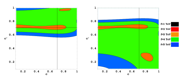
Figure 9: Contour plot of allowed values of $f$ as a function of the angles $c$ and $c^{\prime}$ for $R=0$ and $R=1$ with the 95% C.L. shown.

In Fig. 9 we plot the allowed contour levels at the $95\%$ C.L. for $R=0$, the point where in principle all quadratic divergences could be canceled, and $R=1$ the smallest number of insertions of extra fields required by our “R” rule. We find that for neither $R=0$ or $R=1$ the bounds on this model show significant improvement from the Littlest Higgs model. In the majority of parameter space as can be seen from Fig. 9 the bounds on $f$ are greater than $3$ TeV. This bound is surprising at first since the triplet was shown to have a large influence when we examined the bounds on the Littlest Higgs with gauging only $U(1)_{Y}$. Without the triplet we have no way of canceling off the large $U(1)$ corrections that contribute a shift in $\Delta$ that has the opposite sign of the triplet corrections in the Littlest Higgs. Therefore in the most minimal version of the $SU(6)/Sp(6)$ model it has the same problem as the Littlest Higgs i.e. the large contributions from the $U(1)$ sector of the theory. We do not compute the fine tuning in the $SU(6)/Sp(6)$ model since the contributions to the the Higgs mass depend on a large number of Yukawa couplings that are not constrained as in the Littlest Higgs. In principle the large bound on $f$ does not directly imply a large fine tuning since a choice of parameters could reduce the level of fine tuning however this specific choice of parameter would have to be explained in a UV completion.

4.4 Modifying SU(6)/Sp(6)

Given the relatively strong bounds on $f$ in the “minimal” cases $R=1,0$, we now consider modifying the $U(1)$ sector of the model. In Section 3 we demonstrated the effects of adding an additional $U(1)$ and only gauging $U(1)_{Y}$. With the extra $U(1)$ contribution modification the Littlest Higgs model was slightly improved since the $R=n/5$ rule could be violated, in particular to $R=1/2$ where the light fermions decouple from the heavy $U(1)$ gauge boson. Such special values of $R$ lowered the bounds on $f$ in this variation of the Littlest Higgs model, but only in a rather small region of parameter space. The modification where only $U(1)_{Y}$ was gauged was also not a very significant improvement since the triplet VEV could not be canceled by a contribution from the $U(1)$ sector. The allowed region of parameter space where this modification of the Littlest Higgs model had a low $f$ was again small since it corresponded directly to where the triplet VEV vanished. For $SU(6)/Sp(6)$, if only hypercharge were gauged, there would be minimal corrections to this model in a large region of parameter space since there is no triplet VEV. As before, this leaves open the question of why some of the Higgs quadratic divergences proportional to order one couplings are not canceled (even though they may be numerically not very significant).

Figure 10: Contour plot of allowed values of $f$ as a function of $c$ and $\tan\beta$ for gauging only $U(1)_{Y}$ in the $SU(6)/Sp(6)$ model with the $95\%$ C.L. shown

In Fig. 10 we plot the allowed regions for the $SU(6)/Sp(6)$ model when we gauge only $U(1)_{Y}$. In this case we see a dependence on the value of $\tan\beta$ since the large $U(1)$ corrections do not dominate the fit that we perform as in the minimal $SU(6)/Sp(6)$ case. We see in Fig. 10 that gauging only $U(1)_{Y}$ enlarges the allowed region of parameter space.

In $SU(6)/Sp(6)$ the gauged $U(1)$’s are not subgroups of the global $SU(6)$. Since there is already a portion outside of the the $SU(6)$ we could see the effect of slightly modifying the $U(1)$’s in such a way as to preserve the approximate symmetries they posses while minimizing the bounds on $f$. The way we accomplish this is through doing a $b$ modification as was demonstrated for the Littlest Higgs in Section 3.1. In the case of the $SU(6)/Sp(6)$ model the modification to the bare parameters of the theory involving the $U(1)$ sector scale with a factor $1/(1-8b+48b^{2})$. This scaling can be observed for instance in the $\rho_{*}$ parameter where before

$$\rho_{*}=1+\frac{\Delta}{4}(2-8R+8R^{2}+\cos^{2}2\beta)$$ (4.18)

and with the $b$ modification

$$\rho_{*}=1+\frac{\Delta}{4}\left(\frac{2-8R+8R^{2}}{1-8b+48b^{2}}+\cos^{2}2\beta\right).$$ (4.19)

The modification involving $b$ is important because it allows non-integer values of the $R$ parameter. For the value $b=1/8$, we find $R=1/2$, i.e. the fermions might be decoupled from the heavy $U(1)$ gauge boson.

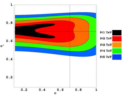
Figure 11: Contour plot of allowed values of $f$ as a function of the angles $c$ and $c^{\prime}$ for $R=1/2$ and $b=1/8$ with the $95\%$ C.L. shown.

In Fig. 11 we demonstrate how using $b=1/8$ to shift $R$ to $1/2$ changes the bounds on $f$ at the $95\%$ C.L.. As one can see from Fig. 11 the bounds on $f$ decrease significantly, analogously to shifting from $R=1$ to $R=1/2$ in the Littlest Higgs model. Comparing the $b$ modification shown in Fig. 11 for the $SU(6)/Sp(6)$ model, and Fig. 6 for the Littlest Higgs model, we see that the $b$ modification opens up a larger region of parameter space for $SU(6)/Sp(6)$ compared to the Littlest Higgs. The difference in allowed parameter regions in the $b$ modification between the Littlest Higgs and the $SU(6)/Sp(6)$ model can be attributed to the non-existence of a triplet in the $SU(6)/Sp(6)$ model. Since there are regions in this model with $f<1$ TeV, to find the precise boundaries one needs to calculate the loop corrections to observables in these regions coming from the heavy top and the extra Higgs fields which is done in [27].

5 SU(4)⁴/SU(3)⁴ Little Higgs

Finally, we consider a recently proposed little Higgs model based on an $SU(4)\times U(1)$ gauge group [8], where $SU(2)_{L}$ is embedded into a simple group instead of $[SU(2)]^{2}$. In this model there is a non-linear sigma model for $[SU(4)/SU(3)]^{4}$ breaking with the diagonal $SU(4)$ subgroup gauged and four non-linear $\sigma$ model fields $\Psi_{i}$ and $\Phi_{i}$ where $i=1,2$. In order to be able to embed quarks into the theory and to reproduce the SM value of $\sin^{2}\theta_{W}$, an additional $U(1)$ group is needed. This model appears to be a fundamentally different type of Little Higgs model when compared to [5, 7] due to the multiple breaking of the global symmetry group by separate “$\Sigma$” fields. This model is a little Higgs since it uses collective symmetries to keep the Higgs a pseudo-Goldstone boson. Instead of using a product group, a simpler group is chosen and multiply broken by four $\Sigma$ fields instead of one large breaking with a single $\Sigma$. In addition, potential terms are added by hand rather than being generated by gauge and Yukawa interactions. This model could be viewed as the reincarnation of the Higgs as a pseudo-Goldstone boson solution of the doublet-triplet splitting problem of SUSY GUTs applied to Little Higgs models [28]. A convenient parameterization of the non-linear $\sigma$ model fields in this model is

$$\Phi_{1}=e^{i\mathcal{H}_{u}\frac{f_{2}}{f_{1}}}\left(\begin{array}[]{c}0\\ 0\\ f_{1}\\ 0\\ \end{array}\right)\;\;\Phi_{2}=e^{-i\mathcal{H}_{u}\frac{f_{1}}{f_{2}}}\left(\begin{array}[]{c}0\\ 0\\ f_{2}\\ 0\\ \end{array}\right)$$ (5.1)

$$\Psi_{1}=e^{i\mathcal{H}_{d}\frac{f_{4}}{f_{3}}}\left(\begin{array}[]{c}0\\ 0\\ 0\\ f_{3}\\ \end{array}\right)\;\;\Psi_{2}=e^{-i\mathcal{H}_{d}\frac{f_{3}}{f_{4}}}\left(\begin{array}[]{c}0\\ 0\\ 0\\ f_{4}\\ \end{array}\right)$$ (5.2)

where

$$\mathcal{H}_{u}=\left(\begin{array}[]{ccc}\begin{array}[]{cc}0&0\\ 0&0\\ \end{array}&h_{u}&\begin{array}[]{c}0\\ 0\end{array}\\ h_{u}^{\dagger}&0&0\\ \begin{array}[]{cc}0&0\end{array}&0&0\end{array}\right)/f_{12}\;\;\mathcal{H}_{d}=\left(\begin{array}[]{ccc}\begin{array}[]{cc}0&0\\ 0&0\\ \end{array}&\begin{array}[]{c}0\\ 0\end{array}&h_{d}\\ \begin{array}[]{cc}0&0\end{array}&0&0\\ h_{d}^{\dagger}&0&0\\ \end{array}\right)/f_{34},$$ (5.3)

and $f_{ij}=\sqrt{f_{i}^{2}+f_{j}^{2}}$. The kinetic term for this model is given by

$$\mathcal{L}_{kinetic}=|\mathcal{D}_{\mu}\Phi_{i}|^{2}+|\mathcal{D}_{\mu}\Psi_{i}|^{2}+[\mbox{fermion and gauge kinetic terms}].$$ (5.4)

where the gauge covariant derivative is

$$\mathcal{D}_{\mu}=(\partial_{\mu}+ig_{4}A_{\mu}^{a}T^{a}-i\frac{g_{X}}{4}A_{\mu}^{X}),$$ (5.5)

and $A_{\mu}^{a},g_{4}$ and $A_{\mu}^{X},g_{X}$ are the gauge bosons and couplings of the $SU(4)$ and $U(1)_{X}$ gauge groups respectively. The diagonal generators for the $SU(4)$ group are

$$T^{3} = 1/2\;\mbox{diag}(1,-1,0,0)~{},$$

$$T^{12} = 1/2\;\mbox{diag}(0,0,1,-1)~{},$$

$$T^{15} = \frac{1}{\sqrt{8}}\;\mbox{diag}(-1,-1,1,1)~{}.$$ (5.6)

Hypercharge is a linear combination of the $U(1)_{X}$ generator and $T^{15}$, $Y=\frac{1}{\sqrt{2}}T^{15}-IX$ where $I$ is the $4$ by $4$ identity matrix and $X$ is the $U(1)_{X}$ charge (for example, the $X$ charge of the quark multiplets must be $5/12$ to give the correct $Y$ charge to $u$ and $d$). The charges of the two Higgs doublet fields under $U(1)_{Y}$ are both $-1/2$ therefore the VEVs of the Higgs fields are of the form

$$\langle h_{u}\rangle=\frac{1}{\sqrt{2}}\left(\begin{array}[]{c}v_{1}\\ 0\end{array}\right)\;\;\langle h_{d}\rangle=\frac{1}{\sqrt{2}}\left(\begin{array}[]{c}v_{2}\\ 0\end{array}\right).$$ (5.7)

We may simplify notation greatly by defining

$$v^{2}=v_{1}^{2}+v_{2}^{2},\;\;\>\>\tan\beta=\frac{v_{2}}{v_{1}},$$ (5.8)

and

$$\tan\gamma=\frac{f_{2}}{f_{1}},\;\;\>\>\tan\eta=\frac{f_{4}}{f_{3}},\;\;\>\>\tan\alpha=\frac{f_{34}}{f_{12}}.$$ (5.9)

Here we choose to make the simplifying assumption $f_{12}=f_{34}=f$. This simplification retains the character of the model with different $f_{i}$’s. however we set the same scale for the VEV’s of the $\Phi$’s and $\Psi$’s. The complete analysis with $f_{12}\neq f_{34}$ is beyond the scope of this paper.

We expand the $\Phi_{i}$’s and $\Psi_{i}$’s to fourth order in the Higgs fields and compute the bare expressions needed to eventually calculate the shifts in the EW precision observables. We make the identification that $g_{4}=g$ the coupling of the SM $SU(2)$ group and

$$g^{\prime}=g_{X}/\sqrt{1+\frac{g_{X}^{2}}{2g^{2}}}~{}.$$ (5.10)

5.1 Contributions to electroweak observables

We find that the relevant bare expressions are

$$M_{W}^{2} = \frac{g^{2}v^{2}}{4}\left[1-\frac{\Delta}{6}\left(\cos^{4}\beta(\tan^{2}\gamma+\cot^{2}\gamma-1)+\sin^{4}\beta(\tan^{2}\eta+\cot^{2}\eta-1)\right)\right]$$

$$M_{Z}^{2} = \frac{(g^{2}+g^{\prime 2})v^{2}}{4}\left[1-\frac{\Delta}{6}\left(\cos^{4}\beta(\tan^{2}\gamma+\cot^{2}\gamma-1)+\sin^{4}\beta(\tan^{2}\eta+\cot^{2}\eta-1)\right)\right.$$

$$\qquad\qquad\qquad\quad\left.-\frac{\Delta}{4}\frac{(g^{2}-g^{\prime 2})^{2}}{g^{4}}\right]$$

$$G_{F} = \frac{1}{\sqrt{2}v^{2}}\left[1+\frac{\Delta}{6}\left(\cos^{4}\beta(\tan^{2}\gamma+\cot^{2}\gamma-1)+\sin^{4}\beta(\tan^{2}\eta+\cot^{2}\eta-1)\right)\right.$$

$$\left.-\frac{\Delta}{2}\left(\cot^{2}\gamma\cos^{2}\beta+\tan^{2}\eta\sin^{2}\beta\right)\right]$$

$$s_{0}^{2} \equiv \sin^{2}\theta_{0}=s_{W}^{2}+\delta s_{W}^{2}=s_{W}^{2}-\frac{s_{W}^{2}c_{W}^{2}}{c_{W}^{2}-s_{W}^{2}}\left[\frac{\delta G_{F}}{G_{F}}+\frac{\delta M_{Z}^{2}}{M_{Z}^{2}}\right]$$ (5.11)

$$= s_{W}^{2}+\frac{s_{W}^{2}c_{W}^{2}}{c_{W}^{2}-s_{W}^{2}}\left[\frac{\Delta}{4}\frac{(g^{2}-g^{\prime 2})^{2}}{g^{4}}+\frac{\Delta}{2}\left(\cot^{2}\gamma\cos^{2}\beta+\tan^{2}\eta\sin^{2}\beta\right)\right],$$

where $\Delta=v^{2}/f^{2}$. We need to identify the photon and neutral current couplings so as to calculate the shift in the couplings of the fermions

$$\mathcal{L}_{\mbox{nc}} = eA_{\mu}J^{\mu}_{Q}+\frac{e}{s_{W}c_{W}}Z_{\mu}\left[J^{3\mu}\left(1+\frac{\Delta}{4}\frac{g^{\prime 2}(g^{2}-g^{\prime 2})}{g^{4}}\right)\right.$$ (5.12)

$$\left.-J^{\mu}_{Q}s_{W}^{2}\left(1+\frac{\Delta}{4}\left(1-\frac{g^{\prime 4}}{g^{4}}\right)\right)+J^{15\mu}\frac{\Delta}{2\sqrt{2}}\left(1-\frac{g^{\prime 2}}{g^{2}}\right)\right]$$

$$-\frac{g^{\prime 4}}{2g^{4}f^{2}}\left(J_{3}^{2}+J_{Q}^{2}\right)-\frac{1}{f^{2}}J_{15}^{2}+\frac{g^{\prime 4}}{f^{2}g^{4}}J_{3}J_{Q}+\frac{\sqrt{2}g^{\prime^{2}}}{g^{2}f^{2}}J_{15}^{\mu}\left(J_{Q\mu}-J_{3\mu}\right)~{}.$$

In addition, we must also calculate the effects of fermion mixing in this model, as $SU(2)$ doublet quarks mix with the heavy singlet quarks. This results in an additional shift of the couplings of the doublet quark mass eigenstates. The Yukawa couplings leading to the fermion mass matrix are given by

$$\mathcal{L}_{\mathrm{quarks}}=\left(\lambda_{1}u_{1}^{c}\Phi_{1}^{\dagger}+\lambda_{2}u_{2}^{c}\Phi_{2}^{\dagger}+\lambda_{3}u_{3}^{c}\Psi_{1}^{\dagger}\right)Q+\frac{\lambda_{d}}{\Lambda^{2}}d^{c}\Phi_{1}\Psi_{1}\Psi_{2}Q+\mathrm{h.c.},$$ (5.13)

where $Q=(q,\chi_{1},\chi_{2})^{T}$. This gives a fermion mass matrix

$$M_{f}=\left(\begin{array}[]{cccc}0&0&0&0\\ 0&0&0&0\\ \lambda_{2}\frac{v}{\sqrt{2}}\cos\beta\cos\gamma&0&\lambda_{2}f_{2}&0\\ \lambda_{3}\frac{v}{\sqrt{2}}\sin\beta\sin\eta&0&0&\lambda_{3}f_{3}\\ \end{array}\right)$$

where we have taken a light quark limit, $\lambda_{d},\lambda_{1}\approx 0$, and ignored CKM mixing. This matrix is diagonalized by a biunitary transformation, of which the physically significant portion is acting on the $SU(4)$ multiplet, mixing the $SU(2)$ doublet quarks with the heavy singlets. This mixing causes a shift in the couplings of the left handed up quarks to the $SU(4)$ gauge bosons. The current interactions can be parametrized by

$$A^{a}_{\mu}J^{a\mu}=A^{a}_{\mu}\bar{Q}\gamma^{\mu}T^{a}Q$$ (5.14)

(no sum over $a$) where $T^{a}$ is the generator corresponding to $A_{\mu}^{a}$. For instance, the $T_{3}$ matrix is given by

$$T^{3}=\left(\begin{array}[]{cccc}1/2&0&0&0\\ 0&-1/2&0&0\\ 0&0&0&0\\ 0&0&0&0\end{array}\right).$$ (5.15)

Equation (5.14) can be rewritten as

$$A^{a}_{\mu}\bar{Q}_{M}UT^{a}U^{\dagger}Q_{M}$$ (5.16)

where $Q_{M}$ are the fermion mass eigenstates, and $U$ is the matrix which rotates $Q$ into this mass eigenbasis. The term involving only the light fermions coming from the $(1,1)$ component of the matrix $UD^{a}U^{\dagger}$ is the standard model coupling of the up-type quarks plus a correction. As an example, this procedure leads to a change in the coupling of the up quarks to the $Z$-boson given by

$$\delta\tilde{g}^{u}_{L}=-\frac{\Delta}{4}\left[\cot^{2}\gamma\cos^{2}\beta+\tan^{2}\eta\sin^{2}\beta\right].$$ (5.17)

The Yukawas for the leptons are similar:

$$\mathcal{L}_{\mathrm{leptons}}=\left(\lambda_{1}^{\nu}\chi_{\nu 1}^{c}\Phi_{2}^{\dagger}+\lambda_{2}^{\nu}\chi_{\nu 2}^{c}\Psi_{1}^{\dagger}\right)L+\frac{\lambda_{e}}{\Lambda^{2}}e^{c}\Phi_{1}\Psi_{1}\Psi_{2}L$$ (5.18)

where $L=(l,\chi_{\nu 1},\chi_{\nu 2})$. Performing the same procedure, one finds that the couplings of the neutrinos to the $Z$ are shifted by exactly the same amount as the up-type quarks. The couplings of the light fermions to the $t_{15}$ gauge bosons are modified in a similar fashion, which would lead to shifts in electromagnetic couplings, but because the charges for the heavy fermions are identical to the up-quark charge, there is no shift. There are also corrections to $J_{15}$ four-fermion operators, but these are higher order in $\Delta$.

The contributions from (5.12) give

$$\delta\tilde{g}^{ff}=\frac{\Delta}{4}\left(1-\tan^{2}\theta_{W}\right)\left[\tan^{2}\theta_{W}(t_{3}^{f}-q^{f})+\sqrt{2}t_{15}^{f}\right]$$ (5.19)

where $t_{15}=-1/\sqrt{8}$ for the left-handed fermions and $0$ for the right-handed fermions.

There are also corrections to the charged current couplings from mass mixing of the light neutrinos and heavy fermions that effectively lead to an additional shift in $G_{F}$. This shift is given by

$$\delta G_{F}=-\frac{1}{\sqrt{2}v^{2}}\frac{\Delta}{2}\left[\cot^{2}\gamma\cos^{2}\beta+\tan^{2}\eta\sin^{2}\beta\right]$$ (5.20)

that was included in the expression for $G_{F}$ in Eq. (5.1) and is the origin of the angle-dependent correction to $s_{0}^{2}$ in Eq. (5.1).

5.2 Four-fermion operators

There are additional four-fermion operators present in this model that were not present in other models due to the presence of the $J^{15}$ currents. To calculate the contributions to the low-energy observables such as atomic parity violation we use a slightly different method than used in [10]. We first integrate out the Z boson and obtain our low energy neutral current Lagrangian

$$\mathcal{L}_{nc} = -\frac{g^{2}+g^{\prime 2}}{2M_{Z}^{2}}\left[J^{3\mu}\left(1+\frac{\Delta}{4}\frac{g^{\prime 2}(g^{2}-g^{\prime 2})}{g^{4}}\right)-J^{\mu}_{Q}s_{W}^{2}\left(1+\frac{\Delta}{4}\left(1-\frac{g^{\prime 4}}{g^{4}}\right)\right)\right.$$ (5.21)

$$\left.{}+J^{15\mu}\frac{\Delta}{2\sqrt{2}}\left(1-\frac{g^{\prime 2}}{g^{2}}\right)\right]^{2}-\frac{g^{\prime 4}}{2g^{4}f^{2}}\left(J_{3}^{2}+J_{Q}^{2}\right)-\frac{1}{f^{2}}J_{15}^{2}$$

$${}+\frac{g^{\prime 4}}{f^{2}g^{4}}J_{3}J_{Q}+\frac{\sqrt{2}g^{\prime^{2}}}{g^{2}f^{2}}J_{15}^{\mu}\left(J_{Q\mu}-J_{3\mu}\right),$$

we then put relevant parts of the Lagrangian in the form

$$\mathcal{L}^{\nu\rm{Hadron}}=-\frac{G_{F}}{\sqrt{2}}\,\bar{\nu}\gamma^{\mu}(1-\gamma^{5})\nu\times\sum_{i}\left[\epsilon_{L}(i)\bar{q}_{i}\gamma^{\mu}(1-\gamma^{5})q_{i}+\epsilon_{R}(i)\bar{q}_{i}\gamma^{\mu}(1+\gamma^{5})q_{i}\right],$$ (5.22)

$$\mathcal{L}^{\nu\rm{e}}=-\frac{G_{F}}{\sqrt{2}}\,\bar{\nu}\gamma^{\mu}(1-\gamma^{5})\nu\,\bar{e}\gamma_{\mu}(g_{V}^{\nu e}-g_{A}^{\nu e}\gamma^{5})e,$$ (5.23)

and

$$\mathcal{L}^{e\rm{Hadron}}=\frac{G_{F}}{\sqrt{2}}\,\times\sum_{i}\left[C_{1i}\bar{e}\gamma_{\mu}\gamma^{5}e\bar{q}_{i}\gamma^{\mu}q_{i}+C_{2i}\bar{e}\gamma_{\mu}e\bar{q}_{i}\gamma^{\mu}\gamma^{5}q_{i}\right].$$ (5.24)

We then use the expressions in [29] to calculate the low energy observables for instance the “weak” charge of heavy atoms is given by

$$Q_{W}=-2\left[C_{1u}(2Z+N)+C_{1d}(Z+2N)\right]$$ (5.25)

where in this model

$$C_{1u}= -\frac{1}{2}+\frac{4}{3}s_{W}^{2}+\frac{2\Delta}{3}s_{W}^{2}\left[2+\cot^{2}\gamma\cos^{2}\beta+\tan^{2}\eta\sin^{2}\beta\right]$$

$$C_{1d}= \left(\frac{1}{2}-\frac{2}{3}s_{W}^{2}\right)\left[1+\frac{\Delta}{2}\left\{2+\cot^{2}\gamma\cos^{2}\beta+\tan^{2}\eta\sin^{2}\beta\right\}\right]$$ (5.26)

once the shift in the couplings due to the fermion mixing has also been taking into account.

The tree level expressions for the low energy observables are then

$$g_{L}^{2}(\nu N\rightarrow\nu X) = \frac{1}{2}-s_{W}^{2}+\frac{5}{9}s_{W}^{4}+\frac{\Delta}{12}(4s_{W}^{2}-3)\left[\cot^{2}\gamma\cos^{2}\beta+\tan^{2}\eta\sin^{2}\beta\right]$$

$$g_{R}^{2}(\nu N\rightarrow\nu X) = \frac{4}{9}s_{W}^{4}$$

$$g_{eA}(\nu e\rightarrow\nu e) = -\frac{1}{2}$$

$$g_{eV}(\nu e\rightarrow\nu e) = -\frac{1}{2}+2s_{W}^{2}$$

$$Q_{W}(\mathrm{Cs}) = -376C_{1u}-422C_{1d},$$ (5.27)

where it is important to note that $s_{W}^{2}$ must be expressed in terms of the observable $s_{0}^{2}$ in (5.1) to obtain the total shift of each parameter.

Direct experimental constraints on other four-fermion operators can also give bounds to little Higgs models. Operators such as

$$\frac{1}{f^{2}}\bar{e}_{L}\gamma_{\mu}e_{L}\bar{q}_{L}\gamma^{\mu}q_{L}$$ (5.28)

coming from the left-left currents in (5.21) can contribute to scattering processes that have stringent bounds which can be found in [30]. The bounds in this particular model are weaker than those coming from the global fit of precision EW data so we will not review them further. Note that these operators arise in all little Higgs models (to date), however we find the bounds from precision electroweak data are stronger than the bounds on these four-fermion operators.

5.3 Numerical results

We compute the bounds on this model using the bare expressions re-expressed in terms of the physical input parameters as done in the previous sections and in [10]. In the general case of $f_{12}\neq f_{34}$ there would be additional mixing between the $Z$, the $Z^{\prime}$, and the gauge boson corresponding to $T^{12}$. One could take into account the angle describing the ratio $f_{12}/f_{34}$ and do another fit, however this adds considerable complexity to the analysis due to mass mixing of heavy gauge eigenstates, and we leave such a study for future exploration.

We compute the bounds for a $95\%$ C.L. which for a $4$ parameter fit corresponds to a $\Delta\chi^{2}=9.49$. The minimum bound on this model at a $95\%$ C.L. is $f=f_{12}=f_{34}=4.2$ TeV, which occurs at $\tan\beta=0.1$, $f_{2}/f_{1}=10$, and $f_{4}/f_{3}=0.1$. Note that we have constrained the ratios of all VEVs to be between 0.1 and 10.

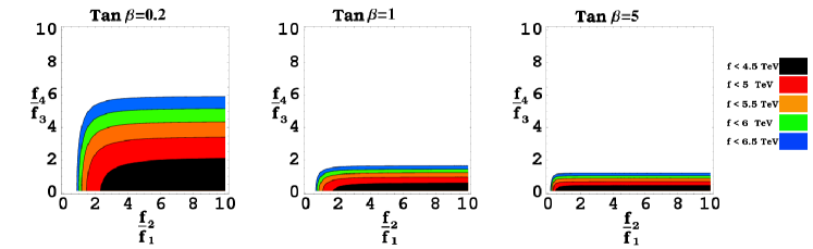
Figure 12: Plot of 95% confidence level values of $f=\sqrt{f_{1}^{2}+f_{2}^{2}}=\sqrt{f_{3}^{2}+f_{4}^{2}}$ as a function of $\tan\beta$, $f_{2}/f_{1}$, and $f_{3}/f_{4}$.

The minimum $\chi^{2}$ per degree of freedom for this model is

$$\frac{\chi^{2}}{\mbox{d.o.f.}}=1.67$$ (5.29)

which we find is worse than the SM with a $115$ GeV Higgs mass, which has $\chi^{2}/\mathrm{d.o.f.}=1.38$. Raising the Higgs mass to $300$ GeV raises the goodness of fit parameter to $\chi^{2}_{300}/\mathrm{d.o.f.}=1.74$ with $m_{H}=300$ GeV, for which $\chi^{2\mathrm{SM}}_{300}/\mathrm{d.o.f.}=1.59$. Overall, the $115$ GeV Higgs is still preferred.

We would like to develop some way of interpreting the bounds on $f$ in terms of a quantification of fine tuning. In order to do this, we calculate the mass of the heavy fermion as a function of the ratio $f_{2}/f_{1}$ and the Yukawa coupling $\lambda_{1}$, fixing $f$ at different values, and setting the top Yukawa $\lambda_{t}=1$ to eliminate $\lambda_{2}$. We choose the best case scenario, $\tan\beta\approx 0$, where there is a larger region of $f$ below $4.5$ TeV. The results are shown in Fig. 13. Therefore there exist regions where $m_{\chi}<f$ and a large $f$ does not directly imply large fine tuning.

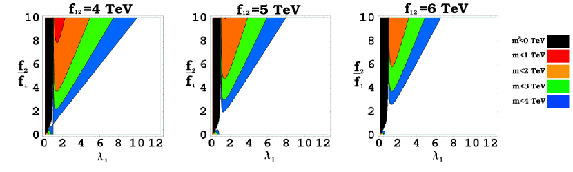
Figure 13: Plot of $m_{\chi}$ as a function of $\lambda_{1}$ and $f_{2}/f_{1}$, with $\tan\beta=0$. The black region corresponds to regions of parameter space that are forbidden due to a negative mass squared for the heavy fermion.

6 Conclusions

We have calculated the tree-level bound on the symmetry breaking scale $f$ in several modifications of the littlest Higgs model. Some of these modifications are motivated by trying to avoid large contributions to EW precision observables. We find that generically $f$ must be larger than several TeV. Non-generically, however, we find the bound on $f$ can be relaxed from $4$ TeV [10] to $1$-$2$ TeV depending on the model variation and the degree of tuning of model parameters. For the $SU(6)/Sp(6)$ model we find that the minimal model has slightly lower bounds than the littlest Higgs, $f>3$ TeV. Interestingly, we showed that a variation of the $SU(6)/Sp(6)$ model exists with a larger region of parameter space where the bound on $f$ is near $1$ TeV. The reason why the $SU(6)/Sp(6)$ can be modified more successfully is because it does not have a Higgs triplet, and because the heavy $U(1)$ gauge boson is somewhat heavier than in the littlest Higgs. The triplet VEV in the littlest Higgs model generically reduces the size of the allowed parameter space even in the case of gauging just $U(1)_{Y}$. The $SU(4)^{4}/SU(3)^{4}$ model is bounded by $f^{2}\equiv f_{1}^{2}+f_{2}^{2}>(4.2\ \mathrm{TeV})^{2}$. In certain models (for example $SU(4)^{4}/SU(3)^{4}$) a large $f$ does not directly imply a large amount of fine tuning since the heavy fermion masses that contribute to the Higgs mass can be lowered below $f$ for a carefully chosen set of parameters.

In general there can be three sources of custodial $SU(2)$ violation in little Higgs models: when light fermions couple to the heavy $U(1)$ gauge boson, when there is an $SU(2)$ triplet that acquires a VEV, or when there are two Higgs doublets with unequal expectation values ($\tan\beta\not=1$). It is interesting that the Littlest Higgs model and the $SU(6)/Sp(6)$ each have a source of custodial $SU(2)$ violation arising from the larger scalar sector of the model with a separate parameter ($a$ in the Littlest Higgs model, $\tan\beta$ in $SU(6)/Sp(6)$) characterizing the size of this contribution. There has also been a interesting recent proposal for a little Higgs model that incorporates an approximate custodial $SU(2)$ symmetry [9], based on a variation of the original minimal moose model [4]. This model is constructed specifically to avoid the gauge contributions to custodial $SU(2)$ violation, although a scalar $SU(2)$ triplet is present which may get an expectation value. We will report on the EW constraints on this model elsewhere [20].

The $SU(4)^{4}/SU(3)^{4}$ model has a qualitatively new feature with respect to EW precision constraints. In this model the quadratically divergent contributions of the Higgs are canceled by gauge bosons mostly in $SU(4)$ that are themselves orthogonal. The absence of mixing of light with heavy gauge bosons is a desirable feature to avoid EW constraints. This is exact for the $SU(2)$ gauge bosons, but only approximate for the $U(1)$ gauge bosons after $SU(4)$ symmetry breaking. In particular, given $f_{12}=f_{34}$, we found that EW precision observables were shifted by an amount proportional to $(g^{2}-g^{\prime 2})/g^{2}$, which characterizes the mixing of the additional $U(1)$ gauge boson with neutral $SU(4)$ gauge bosons. If it had been possible to embed the $U(1)$ into some larger group then with suitably arranged symmetry breaking it is likely that light/heavy gauge boson mixing could be eliminated. (There would still be fermion mixing corrections.) However, to obtain both the proper hypercharges for quarks and leptons as well as the correct weak mixing angle, an additional $U(1)$ was required, and thus mixing between light with heavy $U(1)$ gauge bosons was inevitable. It would be extremely interesting to determine if this can or cannot be avoided in variations of this model.

Finally, several models contain two Higgs doublets that each acquire expectation values. It is well known that if each Higgs couples to both up-type and down-type fermions together (unlike in the minimal supersymmetric standard model, for example), there are additional contributions to flavor changing neutral current processes. Since one motivation of a larger cutoff scale in little Higgs models is to ensure that new four-fermion flavor-violating operators are not strongly constraining, this possible new source of flavor violation must be curtailed. We have already emphasized that a UV completion should determine the viability of the small regions of parameter space where $f$ can be lowered into the $1$-$2$ TeV range. For models with two Higgs doublets, the UV completion should also determine the fermion couplings to the Higgs multiplets. For example, a supersymmetric completion may enforce holomorphic superpotential couplings, thereby avoiding this source of FCNC. It would be very interesting to see what restrictions the absence of new FCNC violating Higgs couplings imposes on the UV completion.

References

-
[1]
LEP Electroweak Working Group, LEPEWWG/2002-01,
http://lepewwg.web.cern.ch/LEPEWWG/stanmod/. - [2] N. Arkani-Hamed, A. G. Cohen and H. Georgi, Phys. Lett. B 513, 232 (2001) [hep-ph/0105239].
- [3] N. Arkani-Hamed, A. G. Cohen, T. Gregoire and J. G. Wacker, JHEP 0208, 020 (2002) [hep-ph/0202089].
- [4] N. Arkani-Hamed, A. G. Cohen, E. Katz, A. E. Nelson, T. Gregoire and J. G. Wacker, JHEP 0208, 021 (2002) [hep-ph/0206020].
- [5] N. Arkani-Hamed, A. G. Cohen, E. Katz and A. E. Nelson, JHEP 0207, 034 (2002) [hep-ph/0206021].
- [6] T. Gregoire and J. G. Wacker, JHEP 0208, 019 (2002) [hep-ph/0206023].
- [7] I. Low, W. Skiba and D. Smith, Phys. Rev. D 66, 072001 (2002) [hep-ph/0207243].
- [8] D. E. Kaplan and M. Schmaltz, hep-ph/0302049.
- [9] S. Chang and J. G. Wacker, hep-ph/0303001.
- [10] C. Csáki, J. Hubisz, G. D. Kribs, P. Meade and J. Terning, hep-ph/0211124.
- [11] J. L. Hewett, F. J. Petriello and T. G. Rizzo, hep-ph/0211218.
- [12] G. Burdman, M. Perelstein and A. Pierce, hep-ph/0212228.
- [13] T. Han, H. E. Logan, B. McElrath and L. T. Wang, hep-ph/0301040.
- [14] C. Dib, R. Rosenfeld and A. Zerwekh, hep-ph/0302068.
- [15] T. Han, H. E. Logan, B. McElrath and L. T. Wang, hep-ph/0302188.
- [16] R. S. Chivukula, N. Evans and E. H. Simmons, Phys. Rev. D 66, 035008 (2002) [hep-ph/0204193].
- [17] R. S. Chivukula, E. H. Simmons and J. Terning, Phys. Lett. B 346, 284 (1995) [hep-ph/9412309].
- [18] C. Csáki, J. Erlich and J. Terning, Phys. Rev. D 66, 064021 (2002), [hep-ph/0203034].
- [19] C. Csáki, J. Erlich, G. D. Kribs and J. Terning, Phys. Rev. D 66, 075008 (2002), [hep-ph/0204109].
- [20] C. Csáki, J. Hubisz, G. D. Kribs, P. Meade, and J. Terning, to appear.
- [21] N. Arkani-Hamed, private communication.
- [22] M. E. Peskin and T. Takeuchi, Phys. Rev. D 46, 381 (1992).
- [23] J. Erler and P. Langacker, review in “The Review of Particle Properties,” K. Hagiwara et al. [Particle Data Group Collaboration], Phys. Rev. D 66, 010001 (2002), updated version online: http://www-pdg.lbl.gov/2001/stanmodelrpp.ps.
- [24] D. C. Kennedy and B. W. Lynn, Nucl. Phys. B 322, 1 (1989); D. C. Kennedy, B. W. Lynn, C. J. Im and R. G. Stuart, Nucl. Phys. B 321, 83 (1989).
- [25] C. P. Burgess, S. Godfrey, H. Konig, D. London and I. Maksymyk, Phys. Rev. D 49, 6115 (1994) [hep-ph/9312291].
- [26] J. Erler, hep-ph/0005084.
- [27] T. Gregoire, D. R. Smith and J. G. Wacker, arXiv:hep-ph/0305275.
- [28] K. Inoue, A. Kakuto and H. Takano, Prog. Theor. Phys. 75, 664 (1986); A. A. Anselm and A. A. Johansen, Phys. Lett. B 200, 331 (1988); Z. G. Berezhiani and G. R. Dvali, Bull. Lebedev Phys. Inst. 5, 55 (1989) [Kratk. Soobshch. Fiz. 5, 42 (1989)]; Z. Berezhiani, C. Csáki and L. Randall, Nucl. Phys. B 444, 61 (1995) [hep-ph/9501336].
- [29] K. Hagiwara et al. [Particle Data Group Collaboration], Phys. Rev. D 66, 010001 (2002).
- [30] K. M. Cheung, Phys. Lett. B 517, 167 (2001), [hep-ph/0106251].