NSF-KITP-03-82
September 2003

Prediction of 𝐔𝐞𝟑subscript𝐔𝐞𝟑\bf U_{e3}

in Neutrino Mass Matrix with Two Zeros

Mizue Honda 111E-mail address: mizue@muse.sc.niigata-u.ac.jp,   Satoru Kaneko 222E-mail address: kaneko@muse.sc.niigata-u.ac.jp

and

Morimitsu Tanimoto 333E-mail address: tanimoto@muse.sc.niigata-u.ac.jp

Department of Physics, Niigata University, Ikarashi 2-8050, 950-2181 Niigata, JAPAN

ABSTRACT


We have discussed predictions of |Ue​3|subscript𝑈𝑒3|U_{e3}| and JC​Psubscriptđœđ¶đ‘ƒJ_{CP} in the framework of the neutrino mass matrix with two zeros. In the case of the best fit values of tan2⁥Ξ12superscript2subscript𝜃12\tan^{2}\theta_{12}, tan2⁥Ξ23superscript2subscript𝜃23\tan^{2}\theta_{23}, Δ​msun2Δsubscriptsuperscript𝑚2sun\Delta m^{2}_{\rm sun} and Δ​matm2Δsuperscriptsubscript𝑚atm2\Delta m_{\rm atm}^{2}, the prediction of |Ue​3|subscript𝑈𝑒3|U_{e3}| is 0.11∌0.14similar-to0.110.140.11\sim 0.14. The lower bound of |Ue​3|subscript𝑈𝑒3|U_{e3}| is 0.050.050.05, which depends on tan⁥Ξ12subscript𝜃12\tan\theta_{12} and tan⁥Ξ23subscript𝜃23\tan\theta_{23}. We have investigated the stability of these predictions taking account of small corrections to zeros, which may come from radiative corrections or off-diagonal elements of the charged lepton mass matrix. The lower bound of |Ue​3|subscript𝑈𝑒3|U_{e3}| comes down considerably due to the small corrections to zeros.

1 Introduction

In recent years empirical understanding of the mass and mixing of neutrinos have been advanced [1, 2, 3]. The KamLAND experiment selected the neutrino mixing solution that is responsible for the solar neutrino problem nearly uniquely [4], only large mixing angle solution. We have now good understanding concerning the neutrino mass difference squared (Δ​matm2Δsubscriptsuperscript𝑚2atm\Delta m^{2}_{\rm atm}, Δ​msun2Δsubscriptsuperscript𝑚2sun\Delta m^{2}_{\rm sun}) and neutrino flavor mixings (sin2⁡2​ξatmsuperscript22subscript𝜃atm\sin^{2}2\theta_{\rm atm}, tan2⁡ξsunsuperscript2subscript𝜃sun\tan^{2}\theta_{\rm sun}) [5]. A constraint has also been placed on the mixing from the reactor experiment of CHOOZ [6].

The texture zeros of the neutrino mass matrix have been discussed to explain these neutrino masses and mixings [7, 8, 9]. Recently, Frampton, Glashow and Marfatia [10] found acceptable textures of the neutrino mass matrix with two independent vanishing entries in the basis of the diagonal charged lepton mass matrix. The KamLAND result has stimulated the phenomenological analyses of the texture zeros [11, 12, 13, 14]. These results favor texture zeros of the neutrino mass matrix phenomenologically.

However, there are theoretical problems. The first one is the effect of radiative corrections. A specific texture of the lepton mass matrix is not preserved to all orders. For example, non-zero components may evolve in zero-entries of the mass matrix at the low energy scale due to radiative corrections even if the zero texture is realized at the high energy scale. The second one is the choice of the flavor basis. In the model with some flavor symmetry, zeros of the neutrino mass matrix are given while the charged lepton mass matrix has off-diagonal components 111There are some models in which zeros of the neutrino mass matrix are realized in the diagonal basis of the charged lepton mass matrix [15, 16, 17].. Then, zeros of the neutrino mass matrix are polluted after diagonalizing the charged lepton mass matrix. Therefore we need to study the stability of predictions of the texture zeros by taking account of small corrections to zeros.

In this paper, we present detailed study of the neutrino mixing parameter Ue​3subscript𝑈𝑒3U_{e3} and CP violating quantity JC​Psubscriptđœđ¶đ‘ƒJ_{CP} [18], which are expected to be affected by the small corrections to zeros in the neutrino mass matrix. It is found that the predicted Ue​3subscript𝑈𝑒3U_{e3} and JC​Psubscriptđœđ¶đ‘ƒJ_{CP} considerably depend on these corrections.

Predictions of the texture two zeros are presented in section 2. Small corrections to zeros are discussed and the stability of predictions are studied in section 3. Section 4 is devoted to the summary.

2 Predictions of texture two zeros

There are 15 textures with two zeros for the effective neutrino mass matrix MÎœsubscript𝑀𝜈M_{\nu}, which have five independent parameters. The two zero conditions give

(MÎœ)a​b=∑i=13Ua​i​Ub​i​λi=0,(MÎœ)α​ÎČ=∑i=13Uα​i​UÎČ​i​λi=0,formulae-sequencesubscriptsubscript𝑀𝜈𝑎𝑏subscriptsuperscript3𝑖1subscript𝑈𝑎𝑖subscript𝑈𝑏𝑖subscript𝜆𝑖0subscriptsubscriptđ‘€đœˆđ›Œđ›œsubscriptsuperscript3𝑖1subscriptđ‘ˆđ›Œđ‘–subscriptđ‘ˆđ›œđ‘–subscript𝜆𝑖0(M_{\nu})_{ab}=\sum^{3}_{i=1}U_{ai}U_{bi}\lambda_{i}=0\ ,\qquad\qquad(M_{\nu})_{\alpha\beta}=\sum^{3}_{i=1}U_{\alpha i}U_{\beta i}\lambda_{i}=0\ , (1)

where λisubscript𝜆𝑖\lambda_{i} is the i-th eigenvalue including the Majorana phases, and indices (a​b)𝑎𝑏(ab) and (α​ÎČ)đ›Œđ›œ(\alpha\beta) denote the flavor components, respectively.

Solving these equations, ratios of neutrino masses m1subscript𝑚1m_{1}, m2subscript𝑚2m_{2}, m3subscript𝑚3m_{3}, which are absolute values of λisubscript𝜆𝑖\lambda_{i}’s, are given in terms of the neutrino mixing matrix U𝑈U [19] as follows:

m1m3subscript𝑚1subscript𝑚3\displaystyle\frac{m_{1}}{m_{3}} =\displaystyle= |Ua​3​Ub​3​Uα​2​UÎČ​2−Ua​2​Ub​2​Uα​3​UÎČ​3Ua​2​Ub​2​Uα​1​UÎČ​1−Ua​1​Ub​1​Uα​2​UÎČ​2|,subscript𝑈𝑎3subscript𝑈𝑏3subscriptđ‘ˆđ›Œ2subscriptđ‘ˆđ›œ2subscript𝑈𝑎2subscript𝑈𝑏2subscriptđ‘ˆđ›Œ3subscriptđ‘ˆđ›œ3subscript𝑈𝑎2subscript𝑈𝑏2subscriptđ‘ˆđ›Œ1subscriptđ‘ˆđ›œ1subscript𝑈𝑎1subscript𝑈𝑏1subscriptđ‘ˆđ›Œ2subscriptđ‘ˆđ›œ2\displaystyle\left|\frac{U_{a3}U_{b3}U_{\alpha 2}U_{\beta 2}-U_{a2}U_{b2}U_{\alpha 3}U_{\beta 3}}{U_{a2}U_{b2}U_{\alpha 1}U_{\beta 1}-U_{a1}U_{b1}U_{\alpha 2}U_{\beta 2}}\right|\ ,
m2m3subscript𝑚2subscript𝑚3\displaystyle\frac{m_{2}}{m_{3}} =\displaystyle= |Ua​1​Ub​1​Uα​3​UÎČ​3−Ua​3​Ub​3​Uα​1​UÎČ​1Ua​2​Ub​2​Uα​1​UÎČ​1−Ua​1​Ub​1​Uα​2​UÎČ​2|.subscript𝑈𝑎1subscript𝑈𝑏1subscriptđ‘ˆđ›Œ3subscriptđ‘ˆđ›œ3subscript𝑈𝑎3subscript𝑈𝑏3subscriptđ‘ˆđ›Œ1subscriptđ‘ˆđ›œ1subscript𝑈𝑎2subscript𝑈𝑏2subscriptđ‘ˆđ›Œ1subscriptđ‘ˆđ›œ1subscript𝑈𝑎1subscript𝑈𝑏1subscriptđ‘ˆđ›Œ2subscriptđ‘ˆđ›œ2\displaystyle\left|\frac{U_{a1}U_{b1}U_{\alpha 3}U_{\beta 3}-U_{a3}U_{b3}U_{\alpha 1}U_{\beta 1}}{U_{a2}U_{b2}U_{\alpha 1}U_{\beta 1}-U_{a1}U_{b1}U_{\alpha 2}U_{\beta 2}}\right|\ . (2)

Then, one can test textures in the ratio RÎœsubscript𝑅𝜈R_{\nu},

RÎœâ‰Ą|m22−m12m32−m22|≈Δ​msun2Δ​matm2,subscript𝑅𝜈subscriptsuperscript𝑚22subscriptsuperscript𝑚21subscriptsuperscript𝑚23subscriptsuperscript𝑚22Δsubscriptsuperscript𝑚2sunΔsubscriptsuperscript𝑚2atm\displaystyle R_{\nu}\equiv\left|\frac{m^{2}_{2}-m^{2}_{1}}{m^{2}_{3}-m^{2}_{2}}\right|\approx\frac{\Delta m^{2}_{\rm sun}}{\Delta m^{2}_{\rm atm}}\ , (3)

which has been given by the experimental data. The ratio RÎœsubscript𝑅𝜈R_{\nu} is given only in terms of four parameters (three mixing angles and one phase) in

U=(c13​c12c13​s12s13​e−i​ή−c23​s12−s23​s13​c12​ei​ήc23​c12−s23​s13​s12​ei​ήs23​c13s23​s12−c23​s13​c12​ei​ή−s23​c12−c23​s13​s12​ei​ήc23​c13),𝑈matrixsubscript𝑐13subscript𝑐12subscript𝑐13subscript𝑠12subscript𝑠13superscript𝑒𝑖𝛿subscript𝑐23subscript𝑠12subscript𝑠23subscript𝑠13subscript𝑐12superscript𝑒𝑖𝛿subscript𝑐23subscript𝑐12subscript𝑠23subscript𝑠13subscript𝑠12superscript𝑒𝑖𝛿subscript𝑠23subscript𝑐13subscript𝑠23subscript𝑠12subscript𝑐23subscript𝑠13subscript𝑐12superscript𝑒𝑖𝛿subscript𝑠23subscript𝑐12subscript𝑐23subscript𝑠13subscript𝑠12superscript𝑒𝑖𝛿subscript𝑐23subscript𝑐13\displaystyle U=\left(\matrix{c_{13}c_{12}&c_{13}s_{12}&s_{13}e^{-i\delta}\cr-c_{23}s_{12}-s_{23}s_{13}c_{12}e^{i\delta}&c_{23}c_{12}-s_{23}s_{13}s_{12}e^{i\delta}&s_{23}c_{13}\cr s_{23}s_{12}-c_{23}s_{13}c_{12}e^{i\delta}&-s_{23}c_{12}-c_{23}s_{13}s_{12}e^{i\delta}&c_{23}c_{13}\cr}\right)\ , (4)

where ci​jsubscript𝑐𝑖𝑗c_{ij} and si​jsubscript𝑠𝑖𝑗s_{ij} denote cos⁡ξi​jsubscript𝜃𝑖𝑗\cos\theta_{ij} and sin⁡ξi​jsubscript𝜃𝑖𝑗\sin\theta_{ij}, respectively.

Seven acceptable textures with two independent zeros were found for the neutrino mass matrix [10], and they have been studied in detail [12, 13] 222Additional two textures may be allowed marginally by current data as shown in ref.[12].. Among them, the textures A1subscript𝐮1A_{1} and A2subscript𝐮2A_{2} of ref.[10], which correspond to the hierarchical neutrino mass spectrum, are strongly favored by the recent phenomenological analyses [11, 12, 13]. Therefore, we study these two textures in this paper.

In the texture A1subscript𝐮1A_{1}, which has two zeros as (MÎœ)e​e=0subscriptsubscript𝑀𝜈𝑒𝑒0(M_{\nu})_{ee}=0 and (MÎœ)e​Ό=0subscriptsubscript𝑀𝜈𝑒𝜇0(M_{\nu})_{e\mu}=0, the mass ratios are given as

m1m3subscript𝑚1subscript𝑚3\displaystyle\frac{m_{1}}{m_{3}} =\displaystyle= |s13c132​(s12​s23c12​c23−s13​e−i​ή)|,subscript𝑠13subscriptsuperscript𝑐213subscript𝑠12subscript𝑠23subscript𝑐12subscript𝑐23subscript𝑠13superscript𝑒𝑖𝛿\displaystyle\left|\frac{s_{13}}{c^{2}_{13}}\left(\frac{s_{12}s_{23}}{c_{12}c_{23}}-s_{13}e^{-i\delta}\right)\right|\ ,
m2m3subscript𝑚2subscript𝑚3\displaystyle\frac{m_{2}}{m_{3}} =\displaystyle= |s13c132​(c12​s23s12​c23+s13​e−i​ή)|.subscript𝑠13subscriptsuperscript𝑐213subscript𝑐12subscript𝑠23subscript𝑠12subscript𝑐23subscript𝑠13superscript𝑒𝑖𝛿\displaystyle\left|\frac{s_{13}}{c^{2}_{13}}\left(\frac{c_{12}s_{23}}{s_{12}c_{23}}+s_{13}e^{-i\delta}\right)\right|\ . (5)

In the texture A2subscript𝐮2A_{2}, which has two zeros as (MÎœ)e​e=0subscriptsubscript𝑀𝜈𝑒𝑒0(M_{\nu})_{ee}=0 and (MÎœ)e​τ=0subscriptsubscript𝑀𝜈𝑒𝜏0(M_{\nu})_{e\tau}=0, the mass ratios are given as

m1m3subscript𝑚1subscript𝑚3\displaystyle\frac{m_{1}}{m_{3}} =\displaystyle= |s13c132​(s12​c23c12​s23+s13​e−i​ή)|,subscript𝑠13subscriptsuperscript𝑐213subscript𝑠12subscript𝑐23subscript𝑐12subscript𝑠23subscript𝑠13superscript𝑒𝑖𝛿\displaystyle\left|\frac{s_{13}}{c^{2}_{13}}\left(\frac{s_{12}c_{23}}{c_{12}s_{23}}+s_{13}e^{-i\delta}\right)\right|\ ,
m2m3subscript𝑚2subscript𝑚3\displaystyle\frac{m_{2}}{m_{3}} =\displaystyle= |s13c132​(c12​c23s12​s23−s13​e−i​ή)|.subscript𝑠13subscriptsuperscript𝑐213subscript𝑐12subscript𝑐23subscript𝑠12subscript𝑠23subscript𝑠13superscript𝑒𝑖𝛿\displaystyle\left|\frac{s_{13}}{c^{2}_{13}}\left(\frac{c_{12}c_{23}}{s_{12}s_{23}}-s_{13}e^{-i\delta}\right)\right|\ . (6)

It is remarked that the mass ratios of the texture A2subscript𝐮2A_{2} are given exactly by replacing tan⁡ξ23subscript𝜃23\tan\theta_{23} in A1subscript𝐮1A_{1} with −cot⁡ξ23subscript𝜃23-\cot\theta_{23}.

If Ξ12subscript𝜃12\theta_{12}, Ξ23subscript𝜃23\theta_{23}, Ξ13subscript𝜃13\theta_{13} and ή𝛿\delta are fixed, we can predict RÎœsubscript𝑅𝜈R_{\nu} of eq.(3), which is compared with the experimental value Δ​msun2/Δ​matm2Δsubscriptsuperscript𝑚2sunΔsubscriptsuperscript𝑚2atm{\Delta m^{2}_{\rm sun}}/{\Delta m^{2}_{\rm atm}}. Taking account of the following data with 90%percent9090\% C.L. [5],

sin2⁥2â€‹ĂŸatm≄0.92,superscript22subscriptitalic-ĂŸatm0.92\displaystyle\sin^{2}2\th_{\rm atm}\geq 0.92\ ,\qquad Δ​matm2=(1.5∌3.9)×10−3​eV2,Δsubscriptsuperscript𝑚2atmsimilar-to1.53.9superscript103superscripteV2\displaystyle\Delta m^{2}_{\rm atm}=(1.5\sim 3.9)\times 10^{-3}{\rm eV}^{2}\ ,
tan2âĄĂŸsun=0.33∌0.67,superscript2subscriptitalic-ĂŸsun0.33similar-to0.67\displaystyle\tan^{2}\th_{\rm sun}=0.33\sim 0.67\ ,\qquad Δ​msun2=(6∌8.5)×10−5​eV2,Δsuperscriptsubscript𝑚sun2similar-to68.5superscript105superscripteV2\displaystyle\Delta m_{\rm sun}^{2}=(6\sim 8.5)\times 10^{-5}{\rm eV}^{2}\ , (7)

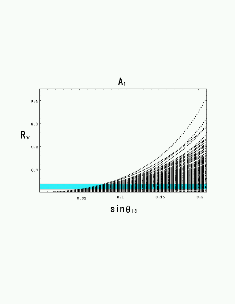
with sinâĄĂŸCHOOZ≀0.2subscriptitalic-ĂŸCHOOZ0.2\sin\th_{\scriptscriptstyle\rm CHOOZ}\leq 0.2, we predict RÎœsubscript𝑅𝜈R_{\nu}. In Fig.1, we present the scatter plot of the predicted RÎœsubscript𝑅𝜈R_{\nu} versus sin⁥Ξ13subscript𝜃13\sin\theta_{13}, in which ή𝛿\delta is taken in the whole range −π∌πsimilar-to𝜋𝜋-\pi\sim\pi for the texture A1subscript𝐮1A_{1}. The parameters are taken in the following ranges of Ξ12=30∘∌39∘subscript𝜃12superscript30similar-tosuperscript39\theta_{12}=30^{\circ}\sim 39^{\circ}, Ξ23=37∘∌53∘subscript𝜃23superscript37similar-tosuperscript53\theta_{23}=37^{\circ}\sim 53^{\circ}, Ξ13=1∘∌12∘subscript𝜃13superscript1similar-tosuperscript12\theta_{13}=1^{\circ}\sim 12^{\circ} and ÎŽ=âˆ’Ï€âˆŒÏ€đ›żđœ‹similar-to𝜋\delta=-\pi\sim\pi. It is found that many predicted values of RÎœsubscript𝑅𝜈R_{\nu} lie outside the experimental allowed region. This result means that there is a strong constraint for the parameter Ξ13subscript𝜃13\theta_{13}. We get sin⁥Ξ13≄0.05subscript𝜃130.05\sin\theta_{13}\geq 0.05 from the experimental value of RÎœsubscript𝑅𝜈R_{\nu} as seen in Fig.1.

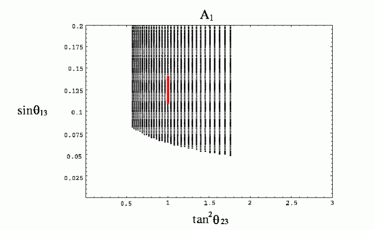
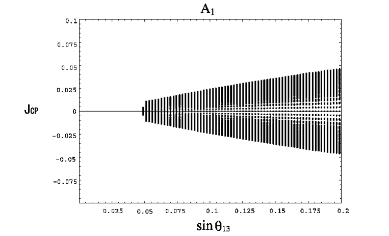
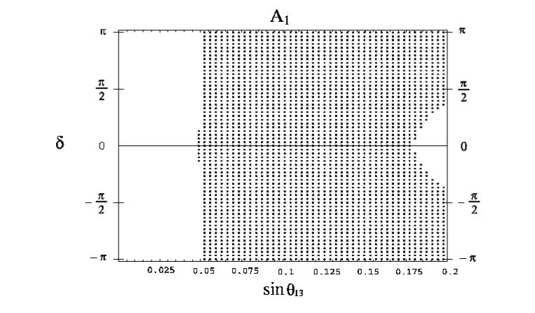
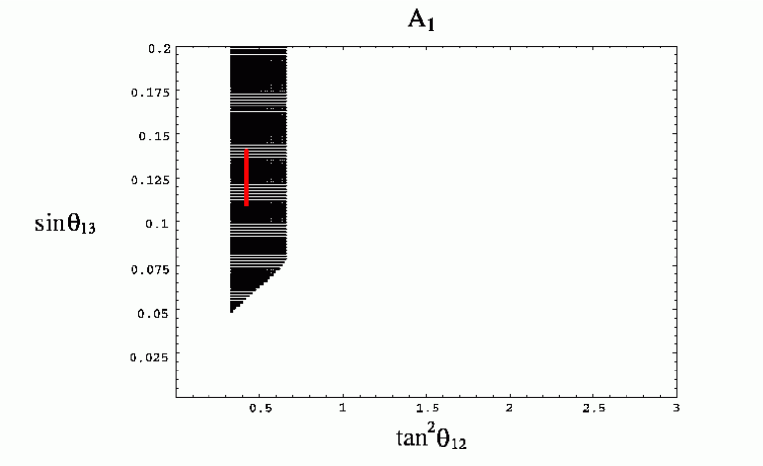
In order to present the allowed region of sin⁥Ξ13subscript𝜃13\sin\theta_{13} for the texture A1subscript𝐮1A_{1}, we show the scatter plot of sin⁥Ξ13subscript𝜃13\sin\theta_{13} versus tan2⁥Ξ12superscript2subscript𝜃12\tan^{2}\theta_{12} and tan2⁥Ξ23superscript2subscript𝜃23\tan^{2}\theta_{23} in Fig.2 and Fig.3, respectively. If we take the best fit values of tan2⁥Ξ12=0.42superscript2subscript𝜃120.42\tan^{2}\theta_{12}=0.42, tan2⁥Ξ23=1superscript2subscript𝜃231\tan^{2}\theta_{23}=1, Δ​msun2=7.3×10⁻⁵​eV2Δsuperscriptsubscript𝑚sun27.3superscript105superscripteV2\Delta m_{\rm sun}^{2}=7.3\times 10^{-5}{\rm eV}^{2} and Δ​matm2=2.5×10⁻³​eV2Δsubscriptsuperscript𝑚2atm2.5superscript103superscripteV2\Delta m^{2}_{\rm atm}=2.5\times 10^{-3}{\rm eV}^{2}, the prediction of sin⁥Ξ13subscript𝜃13\sin\theta_{13} is 0.11∌0.14similar-to0.110.140.11\sim 0.14, where the phase ή𝛿\delta is taken in the whole range −π∌πsimilar-to𝜋𝜋-\pi\sim\pi. In Fig.4, we show JC​Psubscriptđœđ¶đ‘ƒJ_{CP} versus sin⁥Ξ13subscript𝜃13\sin\theta_{13} for the texture A1subscript𝐮1A_{1}. Since JC​Psubscriptđœđ¶đ‘ƒJ_{CP} is proportional to sin⁥Ξ13subscript𝜃13\sin\theta_{13} and sin⁡ή𝛿\sin\delta, we also show the allowed region of ή𝛿\delta versus sin⁥Ξ13subscript𝜃13\sin\theta_{13} in Fig.5. It is found that ή𝛿\delta is allowed in the whole range of −π∌πsimilar-to𝜋𝜋-\pi\sim\pi.

We do not show the numerical results in the texture A2subscript𝐮2A_{2} because those are obtained only by replacing tan⁡ξ23subscript𝜃23\tan\theta_{23} in A1subscript𝐮1A_{1} with −cot⁡ξ23subscript𝜃23-\cot\theta_{23}.

The allowed regions in Fig.2 and Fig.3 are quantitatively understandable in the following approximate relations:

|Ue​3|≡sin⁥Ξ13≃12​tan⁥2​ξ12​cot⁥Ξ23​RΜ​cos⁥2​ξ12,subscript𝑈𝑒3subscript𝜃13similar-to-or-equals122subscript𝜃12subscript𝜃23subscript𝑅𝜈2subscript𝜃12\displaystyle|U_{e3}|\equiv\sin\theta_{13}\simeq\frac{1}{2}\tan 2\theta_{12}\ \cot\theta_{23}\sqrt{R_{\nu}\cos 2\theta_{12}}\ , (8)

for the texture A1subscript𝐮1A_{1}, and

|Ue​3|≡sin⁥Ξ13≃12​tan⁥2​ξ12​tan⁥Ξ23​RΜ​cos⁥2​ξ12,subscript𝑈𝑒3subscript𝜃13similar-to-or-equals122subscript𝜃12subscript𝜃23subscript𝑅𝜈2subscript𝜃12\displaystyle|U_{e3}|\equiv\sin\theta_{13}\simeq\frac{1}{2}\tan 2\theta_{12}\ \tan\theta_{23}\sqrt{R_{\nu}\cos 2\theta_{12}}\ , (9)

for the texture A2subscript𝐮2A_{2}, respectively, where the phase ή𝛿\delta is neglected because it is a next leading term. As tan⁥Ξ12subscript𝜃12\tan\theta_{12} increases, the lower bound of |Ue​3|subscript𝑈𝑒3|U_{e3}| increases, and as tan⁥Ξ23subscript𝜃23\tan\theta_{23} decreases, it increases. It is found in Fig.2 that the lower bound |Ue​3|=0.05subscript𝑈𝑒30.05|U_{e3}|=0.05 is given in the case of the smallest tan2⁥Ξ12superscript2subscript𝜃12\tan^{2}\theta_{12}, while |Ue​3|=0.08subscript𝑈𝑒30.08|U_{e3}|=0.08 is given in the largest tan2⁥Ξ12superscript2subscript𝜃12\tan^{2}\theta_{12}. On the other hand, as seen in Fig.3, the lower bound |Ue​3|=0.05subscript𝑈𝑒30.05|U_{e3}|=0.05 is given in the largest tan2⁥Ξ23superscript2subscript𝜃23\tan^{2}\theta_{23}, while |Ue​3|=0.08subscript𝑈𝑒30.08|U_{e3}|=0.08 is given in the smallest tan2⁥Ξ23superscript2subscript𝜃23\tan^{2}\theta_{23}. The upper bound of |JC​P|subscriptđœđ¶đ‘ƒ|J_{CP}| is 0.050.050.05, but JC​P=0subscriptđœđ¶đ‘ƒ0J_{CP}=0 is still allowed in Fig.4. These predicted regions will be reduced in the future since error bars of experimental data in eq.(7) will be reduced, especially, KamLAND is expected to determine Δ​m122Δsubscriptsuperscript𝑚212\Delta m^{2}_{12} precisely.

3 Stability of predicted 𝐔𝐞𝟑subscript𝐔𝐞𝟑\bf U_{e3}

Above predictions are important ones in the texture zeros. The relative magnitude of each entry of the neutrino mass matrix is roughly given as follows:

MΜ∌(00λ011λ11)for​A1,(0λ0λ11011)for​A2,similar-tosubscript𝑀𝜈matrix00𝜆011𝜆11forsubscript𝐮1matrix0𝜆0𝜆11011forsubscript𝐮2\displaystyle M_{\nu}\sim\left(\matrix{{0}&{0}&\lambda\cr{0}&1&1\cr\lambda&1&1\cr}\right)\ \ \ {\rm for}\ A_{1}\ ,\qquad\qquad\left(\matrix{0&\lambda&0\cr\lambda&1&1\cr 0&1&1\cr}\right)\ \ \ {\rm for}\ A_{2}\ , (10)

where λ≃0.2similar-to-or-equals𝜆0.2\lambda\simeq 0.2. However, these texture zeros are not preserved to all orders. Even if zero-entries of the mass matrix are given at the high energy scale, non-zero components may evolve instead of zeros at the low energy scale due to radiative corrections. Those magnitudes depend on unspecified interactions from which lepton masses are generated. Moreover, zeros of the neutrino mass matrix are given while the charged lepton mass matrix has off-diagonal components in the model with some flavor symmetry. Then, zeros are not realized in the diagonal basis of the charged lepton mass matrix. In other words, zeros of the neutrino mass matrix is polluted by the small off-diagonal elements of the charged lepton mass matrix.

Therefore, one need the careful study of stability of the prediction for |Ue​3|subscript𝑈𝑒3|U_{e3}| and JC​Psubscriptđœđ¶đ‘ƒJ_{CP} because these are small quantities. In order to see the effect of the small non-zero components, the conditions of zeros in eq.(1) are modified. The two conditions turn to

(MÎœ)a​b=∑i=13Ua​i​Ub​i​λi=Ï”,(MÎœ)α​ÎČ=∑i=13Uα​i​UÎČ​i​λi=ω,formulae-sequencesubscriptsubscript𝑀𝜈𝑎𝑏subscriptsuperscript3𝑖1subscript𝑈𝑎𝑖subscript𝑈𝑏𝑖subscript𝜆𝑖italic-Ï”subscriptsubscriptđ‘€đœˆđ›Œđ›œsubscriptsuperscript3𝑖1subscriptđ‘ˆđ›Œđ‘–subscriptđ‘ˆđ›œđ‘–subscript𝜆𝑖𝜔(M_{\nu})_{ab}=\sum^{3}_{i=1}U_{ai}U_{bi}\lambda_{i}=\epsilon\ ,\qquad\qquad(M_{\nu})_{\alpha\beta}=\sum^{3}_{i=1}U_{\alpha i}U_{\beta i}\lambda_{i}=\omega\ , (11)

where Ï”italic-Ï”\epsilon and Ï‰đœ”\omega are arbitrary parameters with the mass unit, which are much smaller than other non-zero components of the mass matrix. These parameters are supposed to be real for simplicity. We get

m1m3subscript𝑚1subscript𝑚3\displaystyle\frac{m_{1}}{m_{3}} =\displaystyle= |U13​U13​U12​U22−U12​U12​U13​U23−U12​U22â€‹Ï”ÂŻ+U12​U12â€‹Ï‰ÂŻU12​U12​U11​U21−U11​U11​U12​U22|,subscript𝑈13subscript𝑈13subscript𝑈12subscript𝑈22subscript𝑈12subscript𝑈12subscript𝑈13subscript𝑈23subscript𝑈12subscript𝑈22ÂŻitalic-Ï”subscript𝑈12subscript𝑈12¯𝜔subscript𝑈12subscript𝑈12subscript𝑈11subscript𝑈21subscript𝑈11subscript𝑈11subscript𝑈12subscript𝑈22\displaystyle\left|\frac{U_{13}U_{13}U_{12}U_{22}-U_{12}U_{12}U_{13}U_{23}-U_{12}U_{22}\overline{\epsilon}+U_{12}U_{12}\overline{\omega}}{U_{12}U_{12}U_{11}U_{21}-U_{11}U_{11}U_{12}U_{22}}\right|\ ,
m2m3subscript𝑚2subscript𝑚3\displaystyle\frac{m_{2}}{m_{3}} =\displaystyle= |U11​U11​U13​U23−U13​U13​U11​U21+U11​U21â€‹Ï”ÂŻâˆ’U11​U11â€‹Ï‰ÂŻU12​U12​U11​U21−U11​U11​U12​U22|,subscript𝑈11subscript𝑈11subscript𝑈13subscript𝑈23subscript𝑈13subscript𝑈13subscript𝑈11subscript𝑈21subscript𝑈11subscript𝑈21ÂŻitalic-Ï”subscript𝑈11subscript𝑈11¯𝜔subscript𝑈12subscript𝑈12subscript𝑈11subscript𝑈21subscript𝑈11subscript𝑈11subscript𝑈12subscript𝑈22\displaystyle\left|\frac{U_{11}U_{11}U_{13}U_{23}-U_{13}U_{13}U_{11}U_{21}+U_{11}U_{21}\overline{\epsilon}-U_{11}U_{11}\overline{\omega}}{U_{12}U_{12}U_{11}U_{21}-U_{11}U_{11}U_{12}U_{22}}\right|\ , (12)

for the texture A1subscript𝐮1A_{1}, and

m1m3subscript𝑚1subscript𝑚3\displaystyle\frac{m_{1}}{m_{3}} =\displaystyle= |U13​U13​U12​U32−U12​U12​U13​U33−U12​U32â€‹Ï”ÂŻ+U12​U12â€‹Ï‰ÂŻU12​U12​U11​U31−U11​U11​U12​U32|,subscript𝑈13subscript𝑈13subscript𝑈12subscript𝑈32subscript𝑈12subscript𝑈12subscript𝑈13subscript𝑈33subscript𝑈12subscript𝑈32ÂŻitalic-Ï”subscript𝑈12subscript𝑈12¯𝜔subscript𝑈12subscript𝑈12subscript𝑈11subscript𝑈31subscript𝑈11subscript𝑈11subscript𝑈12subscript𝑈32\displaystyle\left|\frac{U_{13}U_{13}U_{12}U_{32}-U_{12}U_{12}U_{13}U_{33}-U_{12}U_{32}\overline{\epsilon}+U_{12}U_{12}\overline{\omega}}{U_{12}U_{12}U_{11}U_{31}-U_{11}U_{11}U_{12}U_{32}}\right|\ ,
m2m3subscript𝑚2subscript𝑚3\displaystyle\frac{m_{2}}{m_{3}} =\displaystyle= |U11​U11​U13​U33−U13​U13​U11​U31+U11​U31â€‹Ï”ÂŻâˆ’U11​U11â€‹Ï‰ÂŻU12​U12​U11​U31−U11​U11​U12​U32|,subscript𝑈11subscript𝑈11subscript𝑈13subscript𝑈33subscript𝑈13subscript𝑈13subscript𝑈11subscript𝑈31subscript𝑈11subscript𝑈31ÂŻitalic-Ï”subscript𝑈11subscript𝑈11¯𝜔subscript𝑈12subscript𝑈12subscript𝑈11subscript𝑈31subscript𝑈11subscript𝑈11subscript𝑈12subscript𝑈32\displaystyle\left|\frac{U_{11}U_{11}U_{13}U_{33}-U_{13}U_{13}U_{11}U_{31}+U_{11}U_{31}\overline{\epsilon}-U_{11}U_{11}\overline{\omega}}{U_{12}U_{12}U_{11}U_{31}-U_{11}U_{11}U_{12}U_{32}}\right|\ , (13)

for the texture A2subscript𝐮2A_{2}, where Ï”ÂŻÂŻitalic-Ï”\overline{\epsilon} and Ï‰ÂŻÂŻđœ”\overline{\omega} are normalized ones as Ï”ÂŻ=Ï”/λ3ÂŻitalic-Ï”italic-Ï”subscript𝜆3\overline{\epsilon}=\epsilon/\lambda_{3} and Ï‰ÂŻ=ω/λ3¯𝜔𝜔subscript𝜆3\overline{\omega}=\omega/\lambda_{3}, respectively. We obtain approximately

m1m3subscript𝑚1subscript𝑚3\displaystyle\frac{m_{1}}{m_{3}} ≃similar-to-or-equals\displaystyle\simeq |t12​t23​s13​e−i​ή−t12c23â€‹Ï‰ÂŻ+Ï”ÂŻ|,subscript𝑡12subscript𝑡23subscript𝑠13superscript𝑒𝑖𝛿subscript𝑡12subscript𝑐23¯𝜔¯italic-Ï”\displaystyle\left|t_{12}t_{23}s_{13}e^{-i\delta}-\frac{t_{12}}{c_{23}}\overline{\omega}+\overline{\epsilon}\right|\ ,
m2m3subscript𝑚2subscript𝑚3\displaystyle\frac{m_{2}}{m_{3}} ≃similar-to-or-equals\displaystyle\simeq |1t12​t23​s13​e−i​ή−1t12​c23â€‹Ï‰ÂŻâˆ’Ï”ÂŻ|,1subscript𝑡12subscript𝑡23subscript𝑠13superscript𝑒𝑖𝛿1subscript𝑡12subscript𝑐23¯𝜔¯italic-Ï”\displaystyle\left|\frac{1}{t_{12}}t_{23}s_{13}e^{-i\delta}-\frac{1}{t_{12}c_{23}}\overline{\omega}-\overline{\epsilon}\right|\ , (14)

for the texture A1subscript𝐮1A_{1}, and

m1m3subscript𝑚1subscript𝑚3\displaystyle\frac{m_{1}}{m_{3}} ≃similar-to-or-equals\displaystyle\simeq |−t12​1t23​s13​e−i​ή+t12s23â€‹Ï‰ÂŻ+Ï”ÂŻ|,subscript𝑡121subscript𝑡23subscript𝑠13superscript𝑒𝑖𝛿subscript𝑡12subscript𝑠23¯𝜔¯italic-Ï”\displaystyle\left|-t_{12}\frac{1}{t_{23}}s_{13}e^{-i\delta}+\frac{t_{12}}{s_{23}}\overline{\omega}+\overline{\epsilon}\right|\ ,
m2m3subscript𝑚2subscript𝑚3\displaystyle\frac{m_{2}}{m_{3}} ≃similar-to-or-equals\displaystyle\simeq |−1t12​t23​s13​e−i​ή+1t12​s23â€‹Ï‰ÂŻâˆ’Ï”ÂŻ|,1subscript𝑡12subscript𝑡23subscript𝑠13superscript𝑒𝑖𝛿1subscript𝑡12subscript𝑠23¯𝜔¯italic-Ï”\displaystyle\left|-\frac{1}{t_{12}t_{23}}s_{13}e^{-i\delta}+\frac{1}{t_{12}s_{23}}\overline{\omega}-\overline{\epsilon}\right|\ , (15)

for the texture A2subscript𝐮2A_{2}, where ti​j=tan⁡ξi​jsubscript𝑡𝑖𝑗subscript𝜃𝑖𝑗t_{ij}=\tan\theta_{ij}. We present the approximate expression of |Ue​3|=sin⁡ξ13subscript𝑈𝑒3subscript𝜃13|U_{e3}|=\sin\theta_{13} as follows:

sin⁥Ξ13≃±12​tan⁥2​ξ12​cot⁥Ξ23​RΜ​cos⁥2​ξ12+Ï‰ÂŻâ€‹cos⁥Ύs23+t12t23â€‹Ï”ÂŻâ€‹cos⁥Ύ1−t122+O​(Ï‰ÂŻ2,Ï”ÂŻ2),similar-to-or-equalssubscript𝜃13plus-or-minus122subscript𝜃12subscript𝜃23subscript𝑅𝜈2subscript𝜃12¯𝜔𝛿subscript𝑠23subscript𝑡12subscript𝑡23ÂŻitalic-Ï”đ›ż1subscriptsuperscript𝑡212𝑂superscript¯𝜔2superscriptÂŻitalic-Ï”2\displaystyle\sin\theta_{13}\simeq\pm\frac{1}{2}\tan 2\theta_{12}\ \cot\theta_{23}\sqrt{R_{\nu}\cos 2\theta_{12}}+\frac{\overline{\omega}\ \cos\delta}{s_{23}}+\frac{t_{12}}{t_{23}}\frac{\overline{\epsilon}\ \cos\delta}{1-t^{2}_{12}}+O(\overline{\omega}^{2},\ \overline{\epsilon}^{2})\ , (16)

for the texture A1subscript𝐮1A_{1}, and

sin⁥Ξ13≃±12​tan⁥2​ξ12​tan⁥Ξ23​RΜ​cos⁥2​ξ12+Ï‰ÂŻâ€‹cos⁥Ύc23−t12​t23â€‹Ï”ÂŻâ€‹cos⁥Ύ1−t122+O​(Ï‰ÂŻ2,Ï”ÂŻ2),similar-to-or-equalssubscript𝜃13plus-or-minus122subscript𝜃12subscript𝜃23subscript𝑅𝜈2subscript𝜃12¯𝜔𝛿subscript𝑐23subscript𝑡12subscript𝑡23ÂŻitalic-Ï”đ›ż1subscriptsuperscript𝑡212𝑂superscript¯𝜔2superscriptÂŻitalic-Ï”2\displaystyle\sin\theta_{13}\simeq\pm\frac{1}{2}\tan 2\theta_{12}\ \tan\theta_{23}\sqrt{R_{\nu}\cos 2\theta_{12}}+\frac{\overline{\omega}\ \cos\delta}{c_{23}}-t_{12}t_{23}\frac{\overline{\epsilon}\ \cos\delta}{1-t^{2}_{12}}+O(\overline{\omega}^{2},\ \overline{\epsilon}^{2})\ , (17)

for the texture A2subscript𝐮2A_{2}. In these equations, +(−)+(-) of the first term in the right-hand side corresponds to the case of tan⁡ξ12​tan⁡ξ23>0(<0)subscript𝜃12subscript𝜃23annotated0absent0\tan\theta_{12}\tan\theta_{23}>0(<0). It is remarked that the second and third terms in the right-hand side could be comparable with the first one in eq.(16) and eq.(17).

However, the second and third terms in the right-hand side could be partially canceled each other depending on the sign of tan⁡ξ12subscript𝜃12\tan\theta_{12} and tan⁡ξ23subscript𝜃23\tan\theta_{23}. Therefore, the prediction of |Ue​3|subscript𝑈𝑒3|U_{e3}| is somewhat different between the texture A1subscript𝐮1A_{1} and A2subscript𝐮2A_{2}.

In order to estimate the effect of Ï‰ÂŻÂŻđœ”\overline{\omega} and Ï”ÂŻÂŻitalic-Ï”\overline{\epsilon}, we consider the case in which the charged lepton mass matrix has small off-diagonal components. Suppose that the two zeros in eq.(10) is still preserved for the neutrino sector. The typical model of the charged lepton is the Georgi-Jarlskog texture [20], in which the charged lepton mass matrix MEsubscript𝑀𝐾M_{E} is given as

ME≃(0me​mÎŒ0me​mÎŒmÎŒme​mτ0me​mτmτ),similar-to-or-equalssubscript𝑀𝐾matrix0subscript𝑚𝑒subscript𝑚𝜇0subscript𝑚𝑒subscript𝑚𝜇subscript𝑚𝜇subscript𝑚𝑒subscript𝑚𝜏0subscript𝑚𝑒subscript𝑚𝜏subscript𝑚𝜏M_{E}\simeq\ \left(\matrix{0&\sqrt{m_{e}m_{\mu}}&0\cr\sqrt{m_{e}m_{\mu}}&m_{\mu}&\sqrt{m_{e}m_{\tau}}\cr 0&\sqrt{m_{e}m_{\tau}}&m_{\tau}\cr}\right)\ , (18)

where each matrix element is written in terms of the charged lepton masses, and phases are neglected for simplicity. This matrix is diagonalized by the unitary matrix UEsubscript𝑈𝐾U_{E}, in which the mixing between the first and second families is memΌ≃0.07similar-to-or-equalssubscript𝑚𝑒subscript𝑚𝜇0.07\sqrt{\frac{m_{e}}{m_{\mu}}}\simeq 0.07 and the mixing between the second and third families is memτ≃0.02similar-to-or-equalssubscript𝑚𝑒subscript𝑚𝜏0.02\sqrt{\frac{m_{e}}{m_{\tau}}}\simeq 0.02. Since the neutrino mass matrix is still the texture A1subscript𝐮1A_{1} or the texture A2subscript𝐮2A_{2} 333The combined model with Georgi-Jarlskog texture and the A2subscript𝐮2A_{2} type one is presented in ref.[14], it turns to A1â€Čsuperscriptsubscript𝐮1â€ČA_{1}^{\prime} or A2â€Čsuperscriptsubscript𝐮2â€ČA_{2}^{\prime} as follows:

MΜ∌(Îș2ÎșλÎș11λ11)forA1â€Č,(2​Îș​λλÎșλ11Îș11)forA2â€Č,\displaystyle M_{\nu}\sim\ \ \left(\matrix{\kappa^{2}&\kappa&\lambda\cr\kappa&1&1\cr\lambda&1&1\cr}\right)\quad{\rm for\ }A_{1}^{\prime}\ ,\qquad\left(\matrix{2\kappa\lambda&\lambda&\kappa\cr\lambda&1&1\cr\kappa&1&1\cr}\right)\quad{\rm for\ }A_{2}^{\prime}\ , (19)

in the diagonal basis of the charged lepton mass matrix. Therefore, the parameter Ï”ÂŻÂŻitalic-Ï”\overline{\epsilon} are correlated with Ï‰ÂŻÂŻđœ”\overline{\omega} such as Ï‰ÂŻâ‰ƒÎș/2similar-to-or-equals¯𝜔𝜅2\overline{\omega}\simeq\kappa/2 and Ï”ÂŻâ‰ƒÎș2/2similar-to-or-equalsÂŻitalic-Ï”superscript𝜅22\overline{\epsilon}\simeq\kappa^{2}/2 in the texture A1â€Čsuperscriptsubscript𝐮1â€ČA_{1}^{\prime}, and Ï‰ÂŻâ‰ƒÎș/2similar-to-or-equals¯𝜔𝜅2\overline{\omega}\simeq\kappa/2 and Ï”ÂŻâ‰ƒÎș​λsimilar-to-or-equalsÂŻitalic-Ï”đœ…đœ†\overline{\epsilon}\simeq\kappa\lambda in the texture A2â€Čsuperscriptsubscript𝐮2â€ČA_{2}^{\prime}.

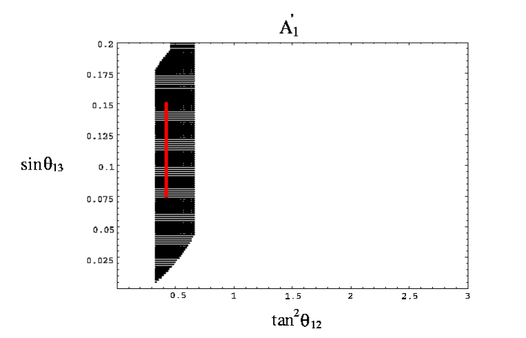
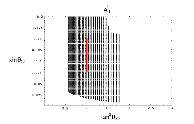
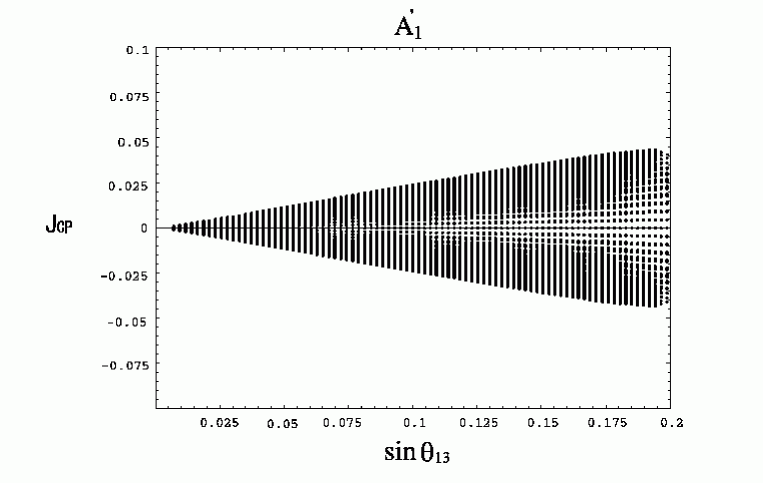
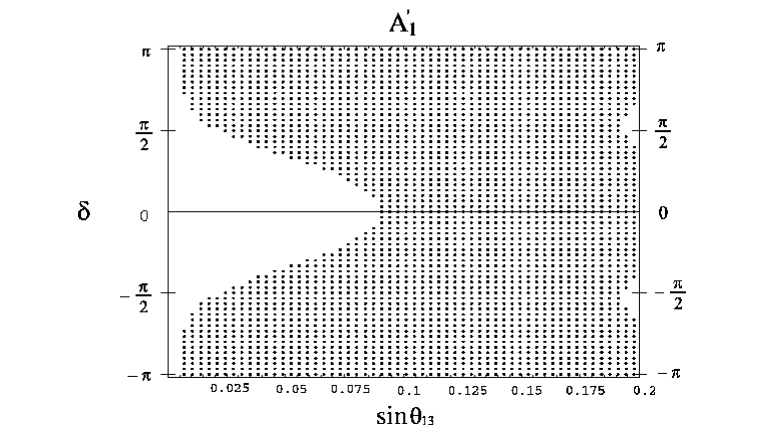
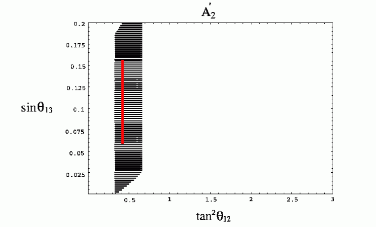
By using the texture A1â€Čsuperscriptsubscript𝐮1â€ČA_{1}^{\prime} of the neutrinos in eq.(19), we show our results of the allowed region of sin⁥Ξ13subscript𝜃13\sin\theta_{13} versus tan2⁥Ξ12superscript2subscript𝜃12\tan^{2}\theta_{12} and tan2⁥Ξ23superscript2subscript𝜃23\tan^{2}\theta_{23} in Fig.6 and Fig.7, respectively, where tan⁥Ξ12subscript𝜃12\tan\theta_{12} and tan⁥Ξ23subscript𝜃23\tan\theta_{23} are taken to be positive. In the case of the best fit values of tan2⁥Ξ12superscript2subscript𝜃12\tan^{2}\theta_{12}, tan2⁥Ξ23superscript2subscript𝜃23\tan^{2}\theta_{23}, Δ​msun2Δsubscriptsuperscript𝑚2sun\Delta m^{2}_{\rm sun} and Δ​matm2Δsuperscriptsubscript𝑚atm2\Delta m_{\rm atm}^{2}, the prediction of sin⁥Ξ13subscript𝜃13\sin\theta_{13} is 0.075∌0.15similar-to0.0750.150.075\sim 0.15, which is somewhat wider than the result of the section 2 due to the correction Îș𝜅\kappa. We have also calculated in the case of tan⁥Ξ12​tan⁥Ξ23<0subscript𝜃12subscript𝜃230\tan\theta_{12}\tan\theta_{23}<0. Predictions are almost same because of Ï‰ÂŻâ‰«Ï”ÂŻmuch-greater-than¯𝜔¯italic-Ï”\overline{\omega}\gg\overline{\epsilon}. In Fig.8, we show JC​Psubscriptđœđ¶đ‘ƒJ_{CP} versus sin⁥Ξ13subscript𝜃13\sin\theta_{13}. We also show the allowed region of ή𝛿\delta versus sin⁥Ξ13subscript𝜃13\sin\theta_{13} in Fig.9. These results should be compared with the ones in Fig.2 ∌similar-to\sim Fig.5. It is noticed that the lower bound of sin⁥Ξ13subscript𝜃13\sin\theta_{13} considerably comes down due to the correction Îș𝜅\kappa. The small |Ue​3|subscript𝑈𝑒3|U_{e3}| of 8×10−38superscript1038\times 10^{-3} is allowed. In Fig.6 and Fig.7, we also find that there is an upper bound on |Ue​3|subscript𝑈𝑒3|U_{e3}| for small values of tan2⁥Ξ12superscript2subscript𝜃12\tan^{2}\theta_{12} and large values of tan2⁥Ξ23superscript2subscript𝜃23\tan^{2}\theta_{23}. We have checked numerically that this upper bound appears due to the higher order terms, which are omitted in eqs.(14), (15), (16) and (17). As seen in Fig.9, the phase ή𝛿\delta is not allowed in the whole range −π∌πsimilar-to𝜋𝜋-\pi\sim\pi if sin⁥Ξ12≀0.09subscript𝜃120.09\sin\theta_{12}\leq 0.09.

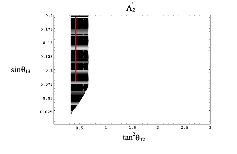
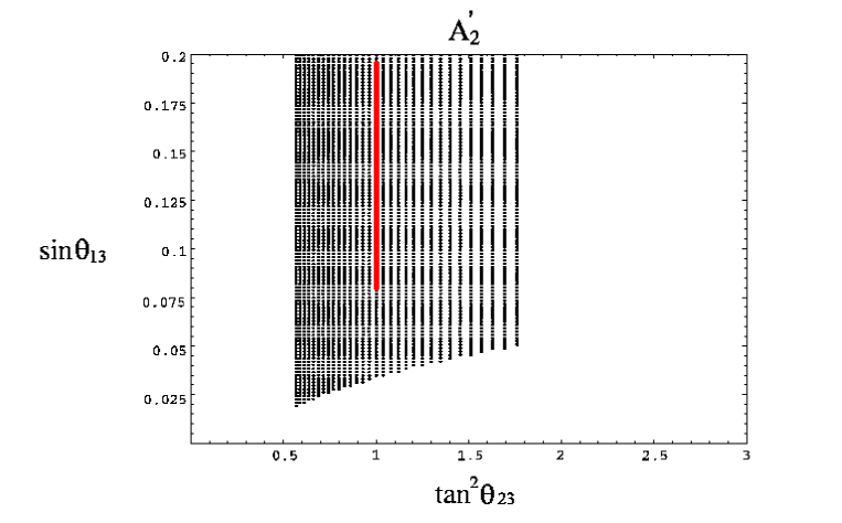
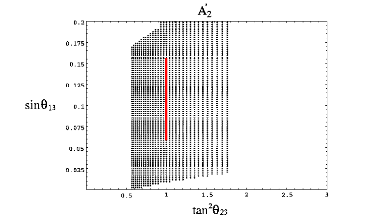
In the texture A2â€Čsuperscriptsubscript𝐮2â€ČA_{2}^{\prime} of eq.(19), we show allowed regions of sin⁥Ξ13subscript𝜃13\sin\theta_{13} versus tan2⁥Ξ12superscript2subscript𝜃12\tan^{2}\theta_{12} and tan2⁥Ξ23superscript2subscript𝜃23\tan^{2}\theta_{23} in Fig.10 and Fig.11, respectively. In the case of the best fit values of tan2⁥Ξ12superscript2subscript𝜃12\tan^{2}\theta_{12}, tan2⁥Ξ23superscript2subscript𝜃23\tan^{2}\theta_{23}, Δ​msun2Δsubscriptsuperscript𝑚2sun\Delta m^{2}_{\rm sun} and Δ​matm2Δsuperscriptsubscript𝑚atm2\Delta m_{\rm atm}^{2}, the prediction of sin⁥Ξ13subscript𝜃13\sin\theta_{13} is 0.08∌0.195similar-to0.080.1950.08\sim 0.195, which is somewhat different from the result of A1â€Čsuperscriptsubscript𝐮1â€ČA_{1}^{\prime}. There is no upper bound on |Ue​3|subscript𝑈𝑒3|U_{e3}| in Fig.10 and Fig.11. The effect of Ï‰ÂŻÂŻđœ”\overline{\omega} is canceled partially by the effect of Ï”ÂŻÂŻitalic-Ï”\overline{\epsilon} as seen in eq.(17). Therefore, allowed regions in Fig.10 and Fig.11 are somewhat different from ones in Fig.6 and Fig.7. We show the result in the case of tan⁥Ξ12​tan⁥Ξ23<0subscript𝜃12subscript𝜃230\tan\theta_{12}\tan\theta_{23}<0 in Fig.12 and Fig.13. The lower bound of sin⁥Ξ13subscript𝜃13\sin\theta_{13} comes down to zero, which is contrasted with the result in Fig.10 and Fig.11 because there is no cancellation between the effect of Ï‰ÂŻÂŻđœ”\overline{\omega} and Ï”ÂŻÂŻitalic-Ï”\overline{\epsilon} as seen in eq.(17). We omit the figure of JC​Psubscriptđœđ¶đ‘ƒJ_{CP} because it is almost same as the result in the case of A1â€Čsuperscriptsubscript𝐮1â€ČA_{1}^{\prime}.

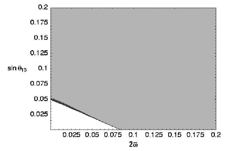
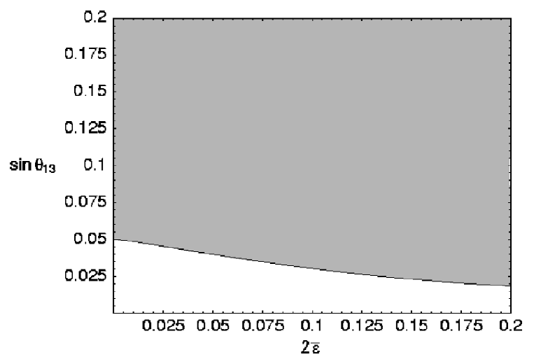
This result depends on a specific model. In order to complete the study of the stability, we also consider the case that two corrections Ï”ÂŻÂŻitalic-Ï”\overline{\epsilon} and Ï‰ÂŻÂŻđœ”\overline{\omega} are independent each other, which may be the case if the deviation from zero arises from radiative corrections. For the texture A1â€Čsuperscriptsubscript𝐮1â€ČA_{1}^{\prime}, we show the allowed region of sin⁥Ξ13subscript𝜃13\sin\theta_{13} versus 2â€‹Ï‰ÂŻ2¯𝜔2\overline{\omega} in Fig.14, where Ï”ÂŻ=0ÂŻitalic-Ï”0\overline{\epsilon}=0 is taken. The gray region is allowed by the experimental data for the texture A1â€Čsuperscriptsubscript𝐮1â€ČA_{1}^{\prime}. The allowed region of the texture A2â€Čsuperscriptsubscript𝐮2â€ČA_{2}^{\prime} is almost same as the one of A1â€Čsuperscriptsubscript𝐮1â€ČA_{1}^{\prime}. In Fig.14, the narrow deep gray region is only added in the case of the texture A2â€Čsuperscriptsubscript𝐮2â€ČA_{2}^{\prime}. We also show the allowed region of sin⁥Ξ13subscript𝜃13\sin\theta_{13} versus Ï”ÂŻÂŻitalic-Ï”\overline{\epsilon} in Fig.15, in which Ï‰ÂŻ=0¯𝜔0\overline{\omega}=0 is taken. There is no difference between the allowed region of both A1â€Čsuperscriptsubscript𝐮1â€ČA_{1}^{\prime} and A2â€Čsuperscriptsubscript𝐮2â€ČA_{2}^{\prime}.

The predicted lower bound of |Ue​3|subscript𝑈𝑒3|U_{e3}| is sensitive to Ï‰ÂŻÂŻđœ”\overline{\omega}. If the correction Ï‰ÂŻÂŻđœ”\overline{\omega} is as large as 0.020.020.02, the lower bound of |Ue​3|subscript𝑈𝑒3|U_{e3}| comes down to 0.0250.0250.025. If Ï‰ÂŻÂŻđœ”\overline{\omega} is larger than 0.040.040.04, the predictability of |Ue​3|subscript𝑈𝑒3|U_{e3}| is lost since |Ue​3|=0subscript𝑈𝑒30|U_{e3}|=0 is allowed. On the other hand, the lower bound is rather insensitive to Ï”ÂŻÂŻitalic-Ï”\overline{\epsilon}. Even if the correction Ï”ÂŻÂŻitalic-Ï”\overline{\epsilon} grows up to be 0.10.10.1, the lower bound of |Ue​3|subscript𝑈𝑒3|U_{e3}| is still 0.020.020.02. It is concluded that the magnitude of the deviation from the zero in the (1,2)/(1,3) element for the texture A1subscript𝐮1A_{1}/A2subscript𝐮2A_{2} is important to predict |Ue​3|subscript𝑈𝑒3|U_{e3}|.

4 Summary

We summarize our results as follows. We have studied |Ue​3|subscript𝑈𝑒3|U_{e3}| and JC​Psubscriptđœđ¶đ‘ƒJ_{CP} in the textures A1subscript𝐮1A_{1} and A2subscript𝐮2A_{2} of the neutrino mass matrix with two zeros. The lower bound of |Ue​3|subscript𝑈𝑒3|U_{e3}| is 0.050.050.05, which considerably depends on tan2⁥Ξ12superscript2subscript𝜃12\tan^{2}\theta_{12} and tan2⁥Ξ23superscript2subscript𝜃23\tan^{2}\theta_{23}. We have investigated the stability of these predictions by taking account of small corrections, which may come from radiative corrections or off-diagonal elements of the charged lepton mass matrix. The lower bound of |Ue​3|subscript𝑈𝑒3|U_{e3}| comes down significantly in the case of Ï‰ÂŻâ‰«0.01much-greater-than¯𝜔0.01\overline{\omega}\gg 0.01, while Ï”ÂŻÂŻitalic-Ï”\overline{\epsilon} is rather insensitive to |Ue​3|subscript𝑈𝑒3|U_{e3}|. Therefore the corrections to the texture zeros in the (1,2)/(1,3) element for the texture A1subscript𝐮1A_{1}/A2subscript𝐮2A_{2} should be carefully taken to predict |Ue​3|subscript𝑈𝑒3|U_{e3}|.

In the case of best fit values of tan2⁥Ξ12superscript2subscript𝜃12\tan^{2}\theta_{12}, tan2⁥Ξ23superscript2subscript𝜃23\tan^{2}\theta_{23}, Δ​msun2Δsubscriptsuperscript𝑚2sun\Delta m^{2}_{\rm sun} and Δ​matm2Δsuperscriptsubscript𝑚atm2\Delta m_{\rm atm}^{2}, the prediction of |Ue​3|subscript𝑈𝑒3|U_{e3}| is 0.075∌0.195similar-to0.0750.1950.075\sim 0.195 even if the corrections are taken into account. This prediction is good news for the near future experiments. The measurement of |Ue​3|subscript𝑈𝑒3|U_{e3}| will be an important test of the texture zeros in the future.


We would like to thank M. Katsumata, H. Nakano and H. So for helpful discussions. We are also grateful to KITP in UCSB, where the paper was completed, for its warm hospitality. This research was supported in part by the National Science Foundation in USA under Grant No. PHY99-07949 and the Grant-in-Aid for Science Research, Ministry of Education, Science and Culture, Japan(No.12047220).
References

  • [1] Super-Kamiokande Collaboration, Y. Fukuda et al, Phys. Rev. Lett. 81 (1998) 1562; ibid. 82 (1999) 2644; ibid. 82 (1999) 5194.
  • [2] Super-Kamiokande Collaboration, S. Fukuda et al. Phys. Rev. Lett. 86, 5651; 5656 (2001).
  • [3] SNO Collaboration: Q. R. Ahmad et al., Phys. Rev. Lett. 87 (2001) 071301;
    nucl-ex/0204008, 0204009.
  • [4] KamLAND Collaboration, K. Eguchi et al., hep-ex/0212021.
  • [5] G. L. Fogli, E. Lisi, M. Marrone, D. Montanino, A. Palazzo and A.M. Rotunno, hep-ph/0212127;
    J. N. Bahcall, M. C. Gonzalez-Garcia and C. Pen~~n\tilde{\rm n}a-Garay, JHEP 0302 (2003) 009;
    M. Maltoni, T. Schwetz and J.W.F. Valle, hep-ph/0212129;
    P.C. Holanda and A. Yu. Smirnov, hep-ph/0212270;
    V. Barger and D. Marfatia, hep-ph/0212126.
  • [6] CHOOZ Collaboration, M. Apollonio et al., Phys. Lett. B466 (1999) 415.
  • [7] H. Nishiura, K. Matsuda and T. Fukuyama, Phys. Rev. D60 (1999) 013006.
  • [8] E. K. Akhmedov, G. C. Branco, M. N. Rebelo, Phys. Rev. Lett. 84 (2000) 3535.
  • [9] S.K. Kang and C.S. Kim, Phys. Rev. D63 (2001) 113010.
  • [10] P.H. Frampton, S.L. Glashow and D. Marfatia, Phys. Lett. B536 (2002) 79.
  • [11] Z. Xing, Phys. Lett. B530 (2002) 159.
  • [12] W. Guo and Z. Xing, hep-ph/0212142.
  • [13] R. Barbieri, T. Hambye and A. Romanino, hep-ph/0302118.
  • [14] M. Bando and M. Obara, hep-ph/0212242, 0302034.
  • [15] A. Zee, Phys. Lett. B93 (1980) 389; B161 (1985) 141;
    L. Wolfenstein, Nucl. Phys. B175 (1980) 92;
    S. T. Petcov, Phys. Lett. B115 (1982) 401;
    C. Jarlskog, M. Matsuda, S. Skadhauge and M. Tanimoto, Phys. Lett. B449 (1999) 240;
    P. H. Frampton and S. Glashow, Phys. Lett. B461 (1999) 95.
  • [16] P.H. Frampton, M.C. Oh and T. Yoshikawa, Phys. Rev. D66 (2002) 033007.
  • [17] A. Kageyama, S. Kaneko, N. Shimoyama and M. Tanimoto, Phys. Lett. B538 (2002) 96.
  • [18] C. Jarlskog, Phys. Rev. Lett. 55 (1985) 1039.
  • [19] Z. Maki, M. Nakagawa and S. Sakata, Prog. Theor. Phys. 28 (1962) 870.
  • [20] H. Georgi and C. Jarlskog, Phys. Lett. B86 (1979) 297.

Refer to caption

Figure 1: Scatter plot of RÎœsubscript𝑅𝜈R_{\nu} versus sin⁥Ξ13subscript𝜃13\sin\theta_{13} for A1subscript𝐮1A_{1}. The unknown phase ή𝛿\delta is taken in the whole range −π∌πsimilar-to𝜋𝜋-\pi\sim\pi. The gray horizontal band is the experimental allowed region.

Refer to caption

Figure 2: Scatter plot of sin⁡ξ13subscript𝜃13\sin\theta_{13} versus tan2⁡ξ12superscript2subscript𝜃12\tan^{2}\theta_{12} for A1subscript𝐮1A_{1}. The best fit is shown by a red line.

Refer to caption

Figure 3: Scatter plot of sin⁡ξ13subscript𝜃13\sin\theta_{13} versus tan2⁡ξ23superscript2subscript𝜃23\tan^{2}\theta_{23} for A1subscript𝐮1A_{1}. The best fit is shown by a red line.

Refer to caption

Figure 4: Scatter plot of JC​Psubscriptđœđ¶đ‘ƒJ_{CP} versus sin⁥Ξ13subscript𝜃13\sin\theta_{13} for A1subscript𝐮1A_{1}.

Refer to caption

Figure 5: Scatter plot of ή𝛿\delta versus sin⁡ξ13subscript𝜃13\sin\theta_{13} for A1subscript𝐮1A_{1}.

Refer to caption


Figure 6: Scatter plot of sin⁥Ξ13subscript𝜃13\sin\theta_{13} versus tan2⁥Ξ12superscript2subscript𝜃12\tan^{2}\theta_{12} in the case of Îș=2â€‹Ï‰ÂŻ=0.07𝜅2¯𝜔0.07\kappa=2\overline{\omega}=0.07 for A1â€Čsuperscriptsubscript𝐮1â€ČA_{1}^{\prime}. The best fit is shown by a red line.

Refer to caption

Figure 7: Scatter plot of sin⁥Ξ13subscript𝜃13\sin\theta_{13} versus tan2⁥Ξ23superscript2subscript𝜃23\tan^{2}\theta_{23} in the case of Îș=2â€‹Ï‰ÂŻ=0.07𝜅2¯𝜔0.07\kappa=2\overline{\omega}=0.07 for A1â€Čsuperscriptsubscript𝐮1â€ČA_{1}^{\prime}. The best fit is shown by a red line.

Refer to caption

Figure 8: Scatter plot of JC​Psubscriptđœđ¶đ‘ƒJ_{CP} versus sin⁥Ξ13subscript𝜃13\sin\theta_{13} in the case of Îș=2â€‹Ï‰ÂŻ=0.07𝜅2¯𝜔0.07\kappa=2\overline{\omega}=0.07 for A1â€Čsuperscriptsubscript𝐮1â€ČA_{1}^{\prime}.

Refer to caption

Figure 9: Scatter plot of ή𝛿\delta versus sin⁥Ξ13subscript𝜃13\sin\theta_{13} for A1â€Čsuperscriptsubscript𝐮1â€ČA_{1}^{\prime}.

Refer to caption


Figure 10: Scatter plot of sin⁥Ξ13subscript𝜃13\sin\theta_{13} versus tan2⁥Ξ12superscript2subscript𝜃12\tan^{2}\theta_{12} in the case of Îș=2â€‹Ï‰ÂŻ=0.07𝜅2¯𝜔0.07\kappa=2\overline{\omega}=0.07 for A2â€Čsuperscriptsubscript𝐮2â€ČA_{2}^{\prime}. The best fit is shown by a red line.

Refer to caption

Figure 11: Scatter plot of sin⁥Ξ13subscript𝜃13\sin\theta_{13} versus tan2⁥Ξ12superscript2subscript𝜃12\tan^{2}\theta_{12} in the case of Îș=2â€‹Ï‰ÂŻ=0.07𝜅2¯𝜔0.07\kappa=2\overline{\omega}=0.07 for A2â€Čsuperscriptsubscript𝐮2â€ČA_{2}^{\prime}. The best fit is shown by a red line.

Refer to caption

Figure 12: Scatter plot of sin⁥Ξ13subscript𝜃13\sin\theta_{13} versus tan2⁥Ξ23superscript2subscript𝜃23\tan^{2}\theta_{23} in the case of tan⁥Ξ12​tan⁥Ξ23<0subscript𝜃12subscript𝜃230\tan\theta_{12}\tan\theta_{23}<0 with Îș=2â€‹Ï‰ÂŻ=0.07𝜅2¯𝜔0.07\kappa=2\overline{\omega}=0.07 for A2â€Čsuperscriptsubscript𝐮2â€ČA_{2}^{\prime}. The best fit is shown by a red line.

Refer to caption

Figure 13: Scatter plot of sin⁥Ξ13subscript𝜃13\sin\theta_{13} versus tan2⁥Ξ23superscript2subscript𝜃23\tan^{2}\theta_{23} in the case of tan⁥Ξ12​tan⁥Ξ23<0subscript𝜃12subscript𝜃230\tan\theta_{12}\tan\theta_{23}<0 with Îș=2â€‹Ï‰ÂŻ=0.07𝜅2¯𝜔0.07\kappa=2\overline{\omega}=0.07 for A2â€Čsuperscriptsubscript𝐮2â€ČA_{2}^{\prime}. The best fit is shown by a red line.

Refer to caption

Figure 14: Prediction of sin⁥Ξ13subscript𝜃13\sin\theta_{13} versus 2â€‹Ï‰ÂŻ2¯𝜔2\overline{\omega} in the case of Ï”ÂŻ=0ÂŻitalic-Ï”0\overline{\epsilon}=0. The gray region is allowed by the experimental data for A1â€Čsuperscriptsubscript𝐮1â€ČA_{1}^{\prime}. The deep gray region is added for A2â€Čsuperscriptsubscript𝐮2â€ČA_{2}^{\prime}.

Refer to caption

Figure 15: Prediction of sin⁥Ξ13subscript𝜃13\sin\theta_{13} versus 2â€‹Ï”ÂŻ2ÂŻitalic-Ï”2\overline{\epsilon} in the case of Ï‰ÂŻ=0¯𝜔0\overline{\omega}=0 for both A1â€Čsuperscriptsubscript𝐮1â€ČA_{1}^{\prime} and A2â€Čsuperscriptsubscript𝐮2â€ČA_{2}^{\prime}. The gray region is allowed by the experimental data.