Large mixing angle solution to the solar neutrino problem and random matter density perturbations

Abstract

There are reasons to believe that mechanisms exist in the solar interior which lead to random density perturbations in the resonant region of the Large Mixing Angle solution to the solar neutrino problem. We find that, in the presence of these density perturbations, the best fit point in the ($\sin^{2}2\theta,\Delta m^{2}$) parameter space moves to smaller values, compared with the values obtained for the standard LMA solution. Combining solar data with KamLAND results, we find a new compatibility region, which we call VERY-LOW LMA, where $\sin^{2}2\theta\approx 0.6$ and $\Delta m^{2}\approx 2\times 10^{-5}$ eV², for random density fluctuations of order $5\%<\xi<8\%$. We argue that such values of density fluctuations are still allowed by helioseismological observations at small scales of order 10 - 1000 km deep inside the solar core.

Assuming CPT invariance, the electronic antineutrino $\bar{\nu}_{e}$ disappearance as well as the neutrino energy spectrum observed in KamLAND [1] are compatible with the predictions based on the Large Mixing Angle (LMA) realization of the MSW mechanism, resonantly enhanced oscillations in matter [2, 3]. This compatibility makes LMA the best solution to the solar neutrino anomaly [4]-[10]. The best fit values of the relevant neutrino parameters which generate such a solution are $\Delta m^{2}=7.3\times 10^{-5}~{}$eV² and $\tan^{2}\theta=0.41$ with a free boron neutrino flux $f_{B}=1.05$ [11] with the 1 $\sigma$ intervals: $\Delta m^{2}=(6.2\leftrightarrow 8.4)\times 10^{-5}~{}$eV² and $\tan^{2}\theta=0.33\leftrightarrow 0.54$.

KamLAND results exclude not only other MSW solutions, such as the small mixing angle realization, but also the just-so solution and the alternative solutions [12] to the solar neutrino problem based on non-standard neutrino interactions [13]-[15], resonant spin-flavor precession in solar magnetic field [16]-[19] and violation of the equivalence principle [20]-[23]. Therefore, the LMA MSW solution appears, for the first time in the solar neutrino problem history, as the unique candidate to explain the anomaly.

Such an agreement of the LMA MSW predictions with the solar neutrino data is achieved assuming the standard approximately exponentially decaying solar matter distribution [24]-[26]. This prediction to the matter distribution inside the sun is very robust since it is in good agreement with helioseismology observations [27].

When doing the fitting of the MSW predictions to the solar neutrino data, it is generally assumed that solar matter do not have any kind of perturbations. I.e., it is assumed that the matter density monotonically decays from the center to the surface of the Sun. There are reasons to believe, nevertheless, that the solar matter density fluctuates around an equilibrium profile. Indeed, in the hydro-dynamical approximation, density perturbations can be induced by temperature fluctuations due to convection of matter between layers with different temperatures. Considering a Boltzman distribution for the matter density, these density fluctuations are found to be around 5% [28]. Another estimation of the level of density perturbations in the solar interior can be given considering the continuity equation up to first order in density and velocity perturbations and the p-modes observations. This analysis leads to a value of density fluctuation around 0.3% [29].

The mechanism that might produce such density fluctuations can also be associated with modes excited by turbulent stress in the convective zone [30] or by a resonance between g-modes and magnetic Alfvèn waves [31]. As the g-modes occur within the solar radiative zone, these resonance creates spikes at specific radii within the Sun. It is not expected that these resonances alter the helioseismic analyses because as they occur deep inside the Sun, they do not affect substantially the observed p-modes. This resonance depends on the density profile and on the solar magnetic field, and as mentioned in Ref. [31], for a magnetic field of order of 10 kG the spacing between the spikes is around 100 km. In the analyses presented in Ref. [31] the values considered for the magnetic field are the ones that satisfy the Chandrasekar limit, which states that the magnetic field energy must be less than the gravitational binding energy.

Considering helioseismology, there are constraints on the density fluctuations, but only those which vary over very long scales, much greater than 1000 km [32, 33, 34]. In particular, the measured spectrum of helioseismic waves is largely insensitive to the existence of density variations whose wavelength is short enough - on scales close to 100 km, deep inside within the solar core - to be of interest for neutrino oscillation, and the amplitude of these perturbations could be large as 10% [31].

So, there is no reason to exclude density perturbations at a few percent level and there are theoretical indications that they really exist.

In the present paper, we study the effect on the Large Mixing Angle parameters when the density matter fluctuates around the equilibrium profile. We consider the case in which these fluctuations are given by a random noise added to an average value. This is a reasonable case, considering that in the lower frequency part of the Fourier spectrum, the p-modes resembles that of noise [28]. Also, considering the resonance of g-modes with Alfvén waves, the superposition of several different modes results in a series of relatively sharp spikes in the radial density profile. The neutrino passing through these spikes fell them as a noisy perturbation whose correlation length is the spacing between the density spikes [31].

Noise fluctuations have been considered in several cases. Loretti and Balantekin [35] have analyzed the effect of a noisy magnetic field and a noisy density. In particular, for a noisy density, they found that the MSW transition is suppressed for a Small Mixing Angle. For the case of strongly adiabatic MSW transitions and large fluctuations, the averaged transition probability saturates at one-half. Refs. [28] and [36] have analyzed the effect of a matter density noise on the MSW effect and found that the presence of noisy matter fluctuations weakens the MSW mechanism, thus reducing the resonant conversion probabilities. These papers, nevertheless, did not take into consideration KamLAND data.

In order to analyze the effect of a noisy density on the neutrino observations, we must consider the evolution equations for the neutrino when the density is given by a main average profile perturbed by a random noisy fluctuation. This is done starting from the standard Schrödinger equation [35, 28].

The evolution for the $\nu_{e}$ - $\nu_{y}$ system is governed by

$$i{\frac{\displaystyle{\ d}}{\displaystyle{\ dr}}}\left(\begin{array}[]{c}\nu_{e}\\ \nu_{y}\end{array}\right)= \left(\begin{array}[]{cc}H_{e}&H_{ey}\\ H_{ey}&H_{y}\end{array}\right)\left(\begin{array}[]{c}\nu_{e}\\ \nu_{y}\end{array}\right),$$ (7)

where

$$H_{e}=2[A_{ey}(t)+\delta A_{ey}],$$ (8)

$$H_{y}=0,~{}H_{ey}\approx{\frac{\Delta m^{2}}{4E}}\sin 2\theta,$$ (9)

$$A_{ey}(t)={\frac{1}{2}}\left[V_{ey}(t)-{\frac{\Delta m^{2}}{4E}}\cos 2\theta\right],$$ (10)

$$\delta A_{ey}(t)\approx\frac{1}{2}V_{ey}(t)\xi.$$ (11)

Here $E$ is the neutrino energy, $\theta$ is the neutrino mixing angle in vacuum, $\Delta m^{2}$ is the neutrino squared mass difference and the matter potential for active-active neutrino conversion reads

$$V_{ey}(t)={\frac{\sqrt{2}G_{F}}{m_{p}}}\rho(t)(1-Y_{n}),$$ (12)

where $V_{ey}$ is the potential, $G_{F}$ is the Fermi constant, $\rho$ is the matter density, $m_{p}$ is the nucleon mass and $Y_{n}$ is the neutron number per nucleon. $\xi$ is the fractional perturbation of the matter potential.

To calculate the survival probability of the neutrinos it is necessary to average the terms of the evolution equation over the random density distribution. Here we assume a delta-correlated Gaussian noise used in Refs. [35, 28]:

$$<\delta A_{ey}^{2n+1}>~{}=0,\\ ~{}<\delta A_{ey}(t)\delta A_{ey}(t_{1})>~{}=2k(t)\delta(t-t_{1}),$$ (13)

where the quantity $k(t)$ is defined by

$$k(t)=~{}<\delta A_{ey}^{2}(t)>L(t)={\frac{1}{2}}V_{ey}^{2}(t)<\xi^{2}>L(t),$$ (14)

where $L(t)$ is the correlation length of the perturbation. The averages, denoted by $<>$, are realized in space for one correlation length, and the delta-correlated noise means that the fluctuations in density are completely spatially uncorrelated for separations larger than one correlation length. $L(t)$ must obey the following relations

$$l_{free}<<L(t)<<\lambda_{m}(t),$$ (15)

where $l_{free}$ is the mean free path of the electrons in the Sun and $\lambda_{m}(t)$ is the characteristic neutrino matter oscillation length.

In order to guarantee that this condition is satisfied in the whole trajectory of the neutrino inside the sun, we assume, following Nunokawa et al. [28], that

$$L(t)=0.1~{}\lambda_{m}(t)=0.1~{}{\frac{2\pi}{\omega(t)}},$$ (16)

where $\omega(t)$ is the frequency of the MSW effect, given by

$$\omega^{2}(t)=4(A^{2}_{ey}(t)+H^{2}_{ey}).$$ (17)

Eqs. (10) and (11) give a value of $L(t)$ between 10 and 100 km in the resonant region for the LMA effect, that is, for the inner part of the Sun.

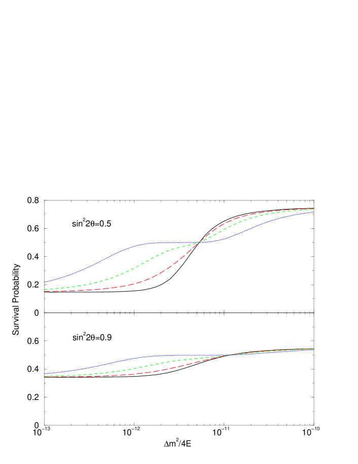
Figure 1: values of the mixing angle, and several values of the perturbation amplitude, $\xi=0\%$ (solid line), $\xi=2\%$ (long dashed line), $\xi=4\%$ (dashed line) and $\xi=8\%$ (dotted line).

We calculate the survival probability of the neutrinos solving the evolution equation, considering the equilibrium density profile given by the Standard Solar Model [26]. The effect of the density noise can be seen in Fig. 1, where the survival probability of the neutrinos is plotted as a function of $\Delta m^{2}/{4E}$ for four values of density perturbation, $\xi=0\%,2\%,4\%$ and $8\%$. We can observe that the effect is amplified when $sin^{2}2\theta=0.5$, rather than when it is $sin^{2}2\theta=0.9$. Considering that the best fit value of $\Delta m^{2}$ obtained from a combined analysis of the solar neutrino data and KamLAND observations is of order $10^{-5}$ eV², we can say that the neutrinos with energy around 10 MeV will be the most affected by the density noise.

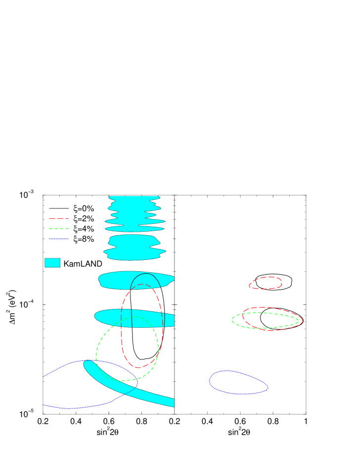
Figure 2: LMA region for different values of the perturbation amplitude, at 95% C.L. for several values of the perturbation amplitude, $\xi=0\%$ (solid line), for $\xi=2\%$ (long dashed line), $\xi=4\%$ (dashed line) and $\xi=8\%$ (dotted line). We also present the allowed region for KamLAND spectral data, for the same C.L.. In the right-handed side of the figure, the combined analysis of both solar neutrino and KamLAND observations is shown.

In Fig. 2 we present the ($\sin^{2}2\theta,\Delta m^{2}$) parameter space comparing the results obtained for solar neutrinos with the allowed regions obtained from KamLAND observations, for four values of density perturbation, $\xi=0\%,2\%,4\%$ and $8\%$. We observe that the values of the parameters $\Delta m^{2}$ and $\sin^{2}2\theta$ that satisfy both the solar neutrinos and KamLAND observations are shifted in the direction of lower values of $\Delta m^{2}$ and $\sin^{2}2\theta$ as the amplitude of the density noise increases. In the left-handed side of Fig. 2, the best fit point of the solar analysis with no perturbations lies in $(\sin^{2}2\theta,\Delta m^{2})=(0.82,7.2\times 10^{-5}{\rm eV}^{2})$, with a minimum $\chi^{2}=65.4$. For $\xi=4\%$, the best fit point goes to $(\sin^{2}2\theta,\Delta m^{2})=(0.71,3.5\times 10^{-5}{\rm eV}^{2})$, with a minimum $\chi^{2}=64.0$, while for $\xi=8\%$ we have $(\sin^{2}2\theta,\Delta m^{2})=(0.33,1.4\times 10^{-5}{\rm eV}^{2})$, with a minimum $\chi^{2}=64.2$. The numbers of degrees of freedom (d.o.f.) in this analysis is 78, obtained from 81 data points, 2 oscillation parameters and $\xi$.

The right-handed side of Fig. 2 shows the combined analysis involving both solar neutrino and KamLAND data. The best fit point of this analysis when no perturbations is assumed lies in $(\sin^{2}2\theta,\Delta m^{2})=(0.85,7.2\times 10^{-5}{\rm eV}^{2})$, with a minimum $\chi^{2}=71.1$. For $\xi=4\%$, our best fit point goes to $(\sin^{2}2\theta,\Delta m^{2})=(0.81,7.2\times 10^{-5}{\rm eV}^{2})$, with a minimum $\chi^{2}=71.5$, while for $\xi=8\%$ we have $(\sin^{2}2\theta,\Delta m^{2})=(0.52,1.9\times 10^{-5}{\rm eV}^{2})$, with a minimum $\chi^{2}=75.5$. Here, the number of d.o.f. is 91 .

The main consequence of introducing random perturbation in the solar matter density is the appearance of entirely new regions in the ($\sin^{2}2\theta\times\Delta m^{2}$) which allow simultaneous compatibility of solar neutrino data and KamLAND observations. Besides the two standard LMA regions, shown in the right-handed side of Fig. 2 by the continuous lines, which were called high and low-LMA in Ref. [11], we find a new region displaced toward smaller values of $\sin^{2}2\theta$ and $\Delta m^{2}$ which we call VERY-low-LMA. There $\Delta m^{2}=(1\leftrightarrow 3)\times 10^{-5}$ eV² and $\sin^{2}2\theta=(0.4\leftrightarrow 0.8)$, at 95% C.L., obtained for $\xi=8\%$.

With no perturbation, the solar data restricts the value of the mixing angle, while the KamLAND data can restrict the value of $\Delta m^{2}$. A combined analysis leads to $\Delta m^{2}=(5\leftrightarrow 9)\times 10^{-5}$ eV² and $sin^{2}2\theta=(0.67\leftrightarrow 0.98)$ at the low-LMA region, and $\Delta m^{2}=(1\leftrightarrow 2)\times 10^{-4}$ eV² and $\sin^{2}2\theta=(0.70\leftrightarrow 0.95)$ at the high-LMA region, at $95\%$ C.L..

Including the effects of random perturbations, the solar data is not able anymore to restrict the value of the mixing angle, and both mixing and $\Delta m^{2}$ are more restricted by the KamLAND data. And, since the LMA regions are displaced to lower values of mixing and $\Delta m^{2}$, the allowed KamLAND region with lower values of $\Delta m^{2}$ becomes important. In fact, such a displacement has already been noticed by Nunokawa et al. [28] without considering the now available data like as zenith spectrum from solar neutrino observations as well as data from KamLAND. Therefore their focus was not only on LMA solution but also small mixing angle parameters with active and sterile neutrinos.

Figure 3: $\chi^{2}$ as a function of $\xi$, the perturbation amplitude, where we minimize in neutrino parameters. Here the number of degrees of freedom is 91.

In Fig. 3 it is shown $\chi^{2}$ as a function of the perturbation amplitude, minimized in $\Delta m^{2}$ and $sin^{2}2\theta$. We can see that even for high values of the perturbation amplitude we still can have a viable solution. We notice that even in a noisy scenario the compatibility of solar neutrino and KamLAND results is still good. In fact, although the absolute best fit of the analysis lies on the non-noise picture where $\xi=0$, we observe that $(\chi^{2}-\chi^{2}_{min})<4$ for $5\%<\xi<8\%$, showing a new scenario of compatibility.

We conclude the paper arguing that random perturbations of the solar matter density will affect the determination of the best fit in the LMA region of the MSW mechanism. Taking into account KamLAND results, the allowed regions of $\Delta m^{2}$ and $sin^{2}2\theta$ at 95% C.L. moves from two distinct regions, the low-LMA and high-LMA, when no noise is assume in the corresponding resonant region, to an entirely new VERY-low-LMA, when a noise amplitude of $5\%<\xi<8\%$ is assumed inside the Sun.

This represents a challenge for the near future confront of solar neutrino data and high-statistic KamLAND observations. If KamLAND will determine $\sin^{2}2\theta<0.5$ and $\Delta m^{2}<4\times 10^{-5}$ eV² it can be necessary to invoke random perturbations in the Sun to recover compatibility with solar neutrino observations.

Note added: After completion of this paper we received two new articles which analyzed similar pictures as ours. One is the Ref. [37] which, differently from its first version [31], included KamLAND data. In this paper a step-function correlated noise has been considered which allows to relax the condition given by Eq. (15). Note that for the LMA parameters, the correlation length obtained from Eq. (15) does not differ very much from the one used in this reference which, therefore, arrive to similar numerical results as ours, summarized in Fig. 3.

Also, a new paper [38] arrived to different conclusions, concerning the quality of the fit for solar neutrino data together with KamLAND data in a noisy scenario.

Acknowlegments: The authors would like to thank FAPESP and CNPq for several financial supports.

References

- [1] K. Eguchi et al., Physical Review Letters 90, 021802 (2003).
- [2] L. Wolfenstein, Phys. Rev. D 17, 2369 (1978).
- [3] S.P. Mikheyev and A. Yu. Smirnov, Yad. Fiz. 42, 1441 (1985) [Sov. J. Nucl. Phys. 42, 913 (1985)], Nuovo Cimento C9, 17 (1986); S.P. Mikheyev and A. Yu. Smirnov, ZHTEF 91 (1986) [Sov. Phys. JETP 64, 4 (1986)].
- [4] T.B. Cleveland et al. (Homestake Collaboration), Astrophys. J. 496, 505 (1998).
- [5] Y. Fukuda et al. (Kamiokande Collaboration), Phys. Rev. Lett. 77, 1683 (1996).
- [6] J.N. Abdurashitov et al. (SAGE Collaboration), Phys. Rev. C 60, 055801 (1999).
- [7] W. Hampel et al. (GALLEX Collaboration), Phys. Lett. B 447, 127 (1999).
- [8] M. Altmann et al. (GNO Collaboration ), Phys. Lett. B 490, 16 (2000).
- [9] Y. Fukuda et al. (Super-Kamiokande Collaboration), Phys. Rev. Lett. 82, 1810 (1999); Phys. Rev. Lett. 86, 5651 (2001).
- [10] (SNO Collaboration) Q. R. Ahmad et al., SNO Collaboration, Phys. Rev. Lett. 87, 071301 (2001); Phys. Rev. Lett. 89, 011301 (2002); Phys. Rev. Lett. 89, 011302 (2002).
- [11] P. C. de Holanda and A. Yu. Smirnov, Journ. of Cosm. and Astropart. Phys. 02, 001 (2003).
- [12] For a detailed list of the references on these solutions see: “Solar Neutrinos: The First Thirty Years”, ed. by R. Davis Jr. et al., Frontiers in Physics, Vol. 92, Addison-Wesley, 1994.
- [13] M.M. Guzzo, A. Masiero and S. T. Petcov, Phys. Lett. B 260, 154 (1991).
- [14] E. Roulet, Phys. Rev. D 44, 935 (1991).
- [15] S. Bergmann, M.M. Guzzo, P.C. de Holanda, P. Krastev and H. Nunokawa, Phys. Rev. D 62, 073001 (2000).
- [16] J. Schechter and J. W. F. Valle, Phys. Rev. 24, 1883 (1981); ibid. 25, 283 (1982).
- [17] C. S. Lim and W. J. Marciano, Phys. Rev. 37, 1368 (1988).
- [18] E. Kh. Akhmedov, Sov. J. Nucl. Phys. 48, 382 (1988); Phys. Lett. B 213, 64 (1988).
- [19] M. M. Guzzo and H. Nunokawa, Astropart. Phys. 12, 87 (1999).
- [20] M. Gasperini, Phys. Rev. D 38, 2635 (1988); ibid. 39, 3606 (1989).
- [21] A. M. Gago, H. Nunokawa and R. Zukanovich Funchal, Phys. Rev. Lett. 84, 4035 (2000); Nucl. Phys. (Proc. Suppl.) B 100, 68 (2001).
- [22] A. Halprin and C. N. Leung, Phys. Rev. Lett. 67, 1833 (1991).
- [23] S. W. Mansour and T. K. Kuo, Phys. Rev. D 60, 097301 (1999); A. Raychaudhuri and A. Sil, hep-ph/0107022.
- [24] J.N. Bahcall, Neutrino Astrophysics, Cambridge University Press, 1989.
- [25] J.N. Bahcall and R.K. Ulrich, Rev. Mod. Phys. 60, 297 (1988); J.N. Bahcall and M.H. Pinsonneault, Rev. Mod. Phys. 64, 885 (1992); S. Turck-Chiéze et al., Astrophys. J. 335, 415 (1988); S. Turck-Chiéze and I. Lopes, Astrophys. J. 408, 347 (1993); V. Castellani, S. Degl’Innocenti and G. Fiorentini, Astron. Astrophys. 271, 601 (1993); V. Castellani et al., Phys. Lett. B 324, 425 (1994); J.N. Bahcall and M.H. Pinsonneault, Rev. Mod. Phys. 67, 781 (1995). J. N. Bahcall, S. Basu and M.H. Pinsonneault, Phys. Lett. B 433, 1 (1998).
- [26] J. N. Bahcall, S. Basu and M.H. Pinsonneault, Astrophys. J. 555, 990 (2001); see also J.N. Bahcall’s home page, http://www.sns.ias.edu/jnb.
-
[27]
J.N. Bahcall, M.H. Pinsonneault, S. Basu and
J. Christensen-Dalsgaard,
Phys. Rev. Lett. 78, 171 (1997). - [28] H. Nunokawa, A. Rossi, V. B. Semikoz, J. W. F. Valle, Nucl. Phys. B 472, 495 (1996).
- [29] S. Turck-Chiéze and I. Lopes, Ap. J 408 (1993) 346; S. Turck-Chiéze et al., Phys. Rep. 230 (1993) 57.
- [30] P. Kumar, E. J. Quataert and J. N Bahcall, Astrophys. Journ. 458, L83 (1996).
- [31] C. Burgess et al., hep-ph/0209094 v1.
- [32] V. Castellani et al, Nucl. Phys. Proc Suppl. 70, 301 (1999).
- [33] J.N. Bahcall, S. Basu and P. Kumar, Astrophys. J., 485 (1997) L91.
- [34] J. Christensen-Dalsgaard, Rev. Mod. Phys. 74 (2003) 1073.
- [35] F. N. Loretti and A. B. Balantekin, Physical Rev D 50, 4762 (1994).
- [36] A. A. Bykov, M. C. Gonzalez-Garcia, C. Peña-Garay, V. Yu Popov, V. B. Semikoz, hep-ph/0005244.
- [37] C. Burgess et al., Astrophys. J., 588 (2003) L65.
- [38] A.B. Balantekin and H. Yüksel, hep-ph/0303169.