The Top Quark, QCD, and New Physics

S. Dawson111This work is supported by the U.S. Department of Energy under contract number DE-AC02-76-CH-00016. Physics Department, Brookhaven National Laboratory,
Upton, NY 11973, USA
dawson@bnl.gov
Abstract

The role of the top quark in completing the Standard Model quark sector is reviewed, along with a discussion of production, decay, and theoretical restrictions on the top quark properties. Particular attention is paid to the top quark as a laboratory for perturbative QCD. As examples of the relevance of QCD corrections in the top quark sector, the calculation of e+ett¯superscript𝑒superscript𝑒𝑡¯𝑡e^{+}e^{-}\rightarrow t{\overline{t}} at next- to-leading-order QCD using the phase space slicing algorithm and the implications of a precision measurement of the top quark mass are discussed in detail. The associated production of a tt¯𝑡¯𝑡t{\overline{t}} pair and a Higgs boson in either e+esuperscript𝑒superscript𝑒e^{+}e^{-} or hadronic collisions is presented at next-to-leading-order QCD and its importance for a measurement of the top quark Yukawa coupling emphasized. Implications of the heavy top quark mass for model builders are briefly examined, with the minimal supersymmetric Standard Model and topcolor discussed as specific examples.

1 Introduction

Long before its discovery in 1995,[1] the top quark was regarded as an essential ingredient of the Standard Model (SM) of particle physics. Its existence, and many of its properties, are determined by requiring the consistency of the Standard Model. These requirements (discussed in Section 2) specify the couplings of the top quark to the SU(3)×SU(2)L×U(1)Y𝑆𝑈3𝑆𝑈subscript2𝐿𝑈subscript1𝑌SU(3)\times SU(2)_{L}\times U(1)_{Y} gauge bosons and many of the top quark properties:

  • Qemt=23esuperscriptsubscript𝑄𝑒𝑚𝑡23delimited-∣∣𝑒Q_{em}^{t}={2\over 3}\mid e\mid

  • Weak isospin partner of b𝑏b quark: T3t=12superscriptsubscript𝑇3𝑡12T_{3}^{t}={1\over 2}

  • Color triplet

  • spin-1212{1\over 2}

The top quark mass, which is measured at CDF and D0 to be Mt=174.3±5.1GeVsubscript𝑀𝑡plus-or-minus174.35.1𝐺𝑒𝑉M_{t}=174.3\pm 5.1~{}GeV,[2] is not predicted in the Standard Model, but is restricted by precision electroweak measurements.[3, 4] In order to confirm that the observed top quark is that predicted by the Standard Model, all of the properties listed above must be experimentally verified by direct observation. Section 3 contains a discussion of the measurements of top quark properties at the Tevatron and surveys the improvements expected at future colliders. Recent reviews of top quark physics can be found in Ref. \refcitetoprevs.

In Section 4, we discuss the top quark as a laboratory for perturbative QCD. At the top quark mass scale, the strong coupling constant is small, αs(Mt)0.1similar-tosubscript𝛼𝑠subscript𝑀𝑡0.1\alpha_{s}(M_{t})\sim 0.1, and so QCD effects involving the top quark are well behaved and we expect a perturbation series in αssubscript𝛼𝑠\alpha_{s} to converge rapidly. The process e+ett¯superscript𝑒superscript𝑒𝑡¯𝑡e^{+}e^{-}\rightarrow t{\overline{t}} provides an example of QCD effects in top quark production and the next-to-leading-order (NLO) QCD corrections are described in detail using the phase space slicing (PSS) algorithm. A knowledge of these higher order QCD corrections is vital for extracting a precise value of the top quark mass from the threshold behavior of the e+ett¯superscript𝑒superscript𝑒𝑡¯𝑡e^{+}e^{-}\rightarrow t{\overline{t}} cross section. As a further example of the role of QCD effects in the top quark sector, we consider the associated production of tt¯h𝑡¯𝑡t{\overline{t}}h and the implications for measuring the top quark Yukawa coupling.

Finally, in Section 5, we discuss the importance of the top quark mass in model building. Since the top quark is heavy, it is expected to play a special role in elucidating the source of fermion masses. We begin by discussing the significance of the top quark in supersymmetric models, and finish with a brief discussion of the top quark and models with dynamical symmetry breaking.

2 Who needs a top quark?

In this section we discuss some of the reasons why the top quark was believed to exist even before its experimental discovery. These considerations fall into three general categories: theoretical consistency of the Standard Model gauge theory (anomaly cancellation), consistency of b𝑏b quark measurements with SM predictions, and consistency of precision measurements with the SM. We then turn to a discussion of top quark production and decay mechanisms at the Tevatron and the LHC.

The particles of the first generation of fermions, along with the Higgs doublet, are shown in Table 2, with their gauge quantum numbers. The third generation is assumed to follow the same pattern, with the left-handed top and bottom quarks forming an SU(2)L𝑆𝑈subscript2𝐿SU(2)_{L} doublet with hypercharge, Y=16𝑌16Y={1\over 6}. The right-handed top and bottom quarks are SU(2)L𝑆𝑈subscript2𝐿SU(2)_{L} singlets. Our normalization is such that:

Qem=T3+Ysubscript𝑄𝑒𝑚subscript𝑇3𝑌Q_{em}=T_{3}+Y (1)

with T3=±12subscript𝑇3plus-or-minus12T_{3}=\pm{1\over 2}.

\tbl

Fermions in the first generation of the Standard Model and their SU(3)×SU(2)L×U(1)Y𝑆𝑈3𝑆𝑈subscript2𝐿𝑈subscript1𝑌SU(3)\times SU(2)_{L}\times U(1)_{Y} quantum numbers. Field SU(3)𝑆𝑈3SU(3) SU(2)L𝑆𝑈subscript2𝐿SU(2)_{L} U(1)Y𝑈subscript1𝑌U(1)_{Y} (uL,dLsubscript𝑢𝐿subscript𝑑𝐿u_{L},d_{L}) 333 222 1616~{}{1\over 6} uRsubscript𝑢𝑅u_{R}, 333 111 2323~{}{2\over 3} dRsubscript𝑑𝑅d_{R}, 333 111 1313-{1\over 3} (νL,eL)subscript𝜈𝐿subscript𝑒𝐿(\nu_{L},e_{L}) 111 222 1212~{}-{1\over 2} eRsubscript𝑒𝑅e_{R} 111 111 11-1 H𝐻{H} 111 222 1212{1\over 2}


2.1 Anomaly Cancellation

The requirement of gauge anomaly cancellation[6, 7] puts restrictions on the couplings of the fermions to vector and axial gauge bosons, denoted here by Vμsuperscript𝑉𝜇V^{\mu} and Aμsuperscript𝐴𝜇A^{\mu}. The fermions of the Standard Model have couplings to the gauge bosons of the general form:

LgAψ¯Tαγμγ5ψAαμ+gVψ¯TαγμψVαμ,similar-to𝐿subscript𝑔𝐴¯𝜓superscript𝑇𝛼subscript𝛾𝜇subscript𝛾5𝜓superscript𝐴𝛼𝜇subscript𝑔𝑉¯𝜓superscript𝑇𝛼subscript𝛾𝜇𝜓superscript𝑉𝛼𝜇{\it L}\sim g_{A}{\overline{\psi}}T^{\alpha}\gamma_{\mu}\gamma_{5}\psi A^{\alpha\mu}+g_{V}{\overline{\psi}}T^{\alpha}\gamma_{\mu}\psi V^{\alpha\mu}, (2)

where Tαsuperscript𝑇𝛼T^{\alpha} is the gauge generator in the adjunct representation. These fermion-gauge boson couplings contribute to triangle graphs of the form shown in Fig. 1. The triangle graphs diverge at high energy,

TabcTr[ηiTa{Tb,Tc}]dnk(2π)n1k3,similar-tosuperscript𝑇𝑎𝑏𝑐𝑇𝑟delimited-[]subscript𝜂𝑖superscript𝑇𝑎superscript𝑇𝑏superscript𝑇𝑐superscript𝑑𝑛𝑘superscript2𝜋𝑛1superscript𝑘3T^{abc}\sim Tr[\eta_{i}T^{a}\{T^{b},T^{c}\}]\int{d^{n}k\over(2\pi)^{n}}{1\over k^{3}}, (3)

where ηi=1subscript𝜂𝑖minus-or-plus1\eta_{i}=\mp 1 for left- and right-handed fermions, ψL,R=12(1γ5)ψsubscript𝜓𝐿𝑅12minus-or-plus1subscript𝛾5𝜓\psi_{L,R}={1\over 2}(1\mp\gamma_{5})\psi. This divergence is independent of the fermion mass and depends only on the fermion couplings to the gauge bosons. Such divergences cannot exist in a physical theory, and must somehow be cancelled. The theory can be anomaly free in a vector-like model where the left- and right-handed particles have identical couplings to gauge bosons and the contribution to Eq. 3 cancels for each pair of particles.

Aaσsubscriptsuperscript𝐴𝜎𝑎A^{\sigma}_{a}Vbμsubscriptsuperscript𝑉𝜇𝑏V^{\mu}_{b}Vcνsubscriptsuperscript𝑉𝜈𝑐V^{\nu}_{c}
Figure 1: Generic Feynman diagram contributing to gauge anomalies. The fermion loop contains all fermions transforming under the gauge symmetry. a,b,c𝑎𝑏𝑐a,b,c are gauge indices.

From Table 1, however, it is clear that the Standard Model is not vector-like. The anomaly, Tabcsuperscript𝑇𝑎𝑏𝑐T^{abc}, must therefore be cancelled by a judicious choice of fermion representations under the various gauge groups.

The only non-vanishing contribution to the anomaly in the Standard Model is from

ΣTr[Y{Ta,Tb}],Σ𝑇𝑟delimited-[]𝑌superscript𝑇𝑎superscript𝑇𝑏\Sigma Tr[Y\{T^{a},T^{b}\}], (4)

where Tasuperscript𝑇𝑎T^{a} are the SU(2)L𝑆𝑈subscript2𝐿SU(2)_{L} generators and the sum is over all fermions in the theory. Eq. 4 vanishes for the hypercharge assignments given in Table 1. Note that the anomaly cancels separately for each generations of fermions. The cancellation of the gauge anomalies in the Standard Model for the third generation therefore requires that the b𝑏b quark have a T3=12subscript𝑇312T_{3}={1\over 2} partner with electric charge Qemt=23esuperscriptsubscript𝑄𝑒𝑚𝑡23delimited-∣∣𝑒Q_{em}^{t}={2\over 3}\mid e\mid, and hypercharge Yt=QemtT3tsuperscript𝑌𝑡subscriptsuperscript𝑄𝑡𝑒𝑚superscriptsubscript𝑇3𝑡Y^{t}=Q^{t}_{em}-T_{3}^{t}. The partner of the b𝑏b quark is by definition the top quark. Since anomaly cancellation is independent of mass, a𝑝𝑟𝑖𝑜𝑟𝑖𝑎𝑝𝑟𝑖𝑜𝑟𝑖{\it a~{}priori}, the top quark mass could be anything.

2.2 b𝑏b quark properties

Many of the experimental properties of the b𝑏b quark require that it be a T3b=12superscriptsubscript𝑇3𝑏12T_{3}^{b}=-{1\over 2} particle with Qemb=13superscriptsubscript𝑄𝑒𝑚𝑏13Q_{em}^{b}=-{1\over 3} and Yb=16superscript𝑌𝑏16Y^{b}={1\over 6}. The coupling of the b𝑏b quark to the Z𝑍Z boson can be tested to check if it has these quantum numbers. The SM fermions couple to the Z𝑍Z boson as,

L=g4cosθWψ¯γμ[Ri(1+γ5)+Li(1γ5)]ψiZμ,𝐿𝑔4subscript𝜃𝑊¯𝜓subscript𝛾𝜇delimited-[]subscript𝑅𝑖1subscript𝛾5subscript𝐿𝑖1subscript𝛾5subscript𝜓𝑖superscript𝑍𝜇{\it L}=-{g\over 4\cos\theta_{W}}{\overline{\psi}}\gamma_{\mu}\biggl{[}R_{i}(1+\gamma_{5})+L_{i}(1-\gamma_{5})\biggr{]}\psi_{i}Z^{\mu}~{}, (5)

where

Risubscript𝑅𝑖\displaystyle R_{i} =\displaystyle= 2Qisin2θW2subscript𝑄𝑖superscript2subscript𝜃𝑊\displaystyle-2Q_{i}\sin^{2}\theta_{W}
Lisubscript𝐿𝑖\displaystyle L_{i} =\displaystyle= 2T3i2Qisin2θW,2subscript𝑇3𝑖2subscript𝑄𝑖superscript2subscript𝜃𝑊\displaystyle 2T_{3i}-2Q_{i}\sin^{2}\theta_{W}~{}, (6)

and θWsubscript𝜃𝑊\theta_{W} is the electroweak mixing angle. The experimental value of Rhadsubscript𝑅𝑎𝑑R_{had} is sensitive to Qembsuperscriptsubscript𝑄𝑒𝑚𝑏Q_{em}^{b},

Rhadσ(e+ehadrons)σ(e+eμ+μ).subscript𝑅𝑎𝑑𝜎superscript𝑒superscript𝑒hadrons𝜎superscript𝑒superscript𝑒superscript𝜇superscript𝜇R_{had}\equiv{\sigma(e^{+}e^{-}\rightarrow{\hbox{hadrons}})\over\sigma(e^{+}e^{\rightarrow}\mu^{+}\mu^{-})}~{}. (7)

At a center-of-mass energy, s=2mb𝑠2subscript𝑚𝑏\sqrt{s}=2m_{b}, Rbsubscript𝑅𝑏R_{b} depends sensitively on the b𝑏b quark electric charge,

δRhad(2mb)=Nc(Qb)2+O(αs),𝛿subscript𝑅𝑎𝑑2subscript𝑚𝑏subscript𝑁𝑐superscriptsubscript𝑄𝑏2𝑂subscript𝛼𝑠\delta R_{had}(2m_{b})=N_{c}(Q_{b})^{2}+{\it O}(\alpha_{s}), (8)

where Nc=3subscript𝑁𝑐3N_{c}=3 is the number of colors. The experimental measurement,[8]

δRhad(2mb)=.36±.09±.03𝛿subscript𝑅𝑎𝑑2subscript𝑚𝑏plus-or-minus.36.09.03\delta R_{had}(2m_{b})=.36\pm.09\pm.03 (9)

is in good agreement with the theoretical prediction from Qemb=13subscriptsuperscript𝑄𝑏𝑒𝑚13Q^{b}_{em}=-{1\over 3}, verifying the SM electric charge assignment of the b𝑏b quark.

Similarly, the SU(2)L𝑆𝑈subscript2𝐿SU(2)_{L} quantum numbers of the left- and right- handed b𝑏b quarks are probed by the decay rate for Z𝑍Z to bb¯𝑏¯𝑏b{\overline{b}} quark pairs. If the b𝑏b did not have a top quark partner, it would be an isospin 00 particle (T3b=0superscriptsubscript𝑇3𝑏0T_{3}^{b}=0) and the decay width would be dramatically different from that of the SM. The decay width is given in terms of the left and right- handed couplings of the Z𝑍Z to the bb¯𝑏¯𝑏b{\overline{b}} pair,[9]

Γ(Zbb¯)=GFMZ342π(Lb2+Rb2).Γ𝑍𝑏¯𝑏subscript𝐺𝐹superscriptsubscript𝑀𝑍342𝜋superscriptsubscript𝐿𝑏2superscriptsubscript𝑅𝑏2\Gamma(Z\rightarrow b{\overline{b}})={G_{F}M_{Z}^{3}\over 4\sqrt{2}\pi}(L_{b}^{2}+R_{b}^{2}). (10)

If the b𝑏b quark were an isospin singlet, then the decay width would be changed,

Γ(Zbb¯)T3b=12Γ(Zbb¯)T3b=0Γsuperscript𝑍𝑏¯𝑏superscriptsubscript𝑇3𝑏12Γsuperscript𝑍𝑏¯𝑏superscriptsubscript𝑇3𝑏0\displaystyle{\Gamma(Z\rightarrow b{\overline{b}})^{T_{3}^{b}=-{1\over 2}}\over\Gamma(Z\rightarrow b{\overline{b}})^{T_{3}^{b}=0}} =\displaystyle= 1+4Qbsin2θW+8Qb2sin4θW8Qb2sin4θW14subscript𝑄𝑏superscript2subscript𝜃𝑊8superscriptsubscript𝑄𝑏2superscript4subscript𝜃𝑊8superscriptsubscript𝑄𝑏2superscript4subscript𝜃𝑊\displaystyle{1+4Q_{b}\sin^{2}\theta_{W}+8Q_{b}^{2}\sin^{4}\theta_{W}\over 8Q_{b}^{2}\sin^{4}\theta_{W}}
similar-to\displaystyle\sim 13.13\displaystyle 13\quad.

The measurement of the Zbb¯𝑍𝑏¯𝑏Z\rightarrow b{\overline{b}} decay width excludes the T3b=0superscriptsubscript𝑇3𝑏0T_{3}^{b}=0 hypothesis for the b𝑏b quark.[3]

  • The measured b𝑏b couplings, combined with anomaly cancelation, require that the b𝑏b quark have a T3t=12superscriptsubscript𝑇3𝑡12T_{3}^{t}={1\over 2}, color triplet, fermion partner: this is the top quark.

2.3 Precision Measurements

Before the top quark was discovered, an approximate value for its mass was known from precision measurements, which depend sensitively on the top quark mass. At tree level, all electroweak measurements depend on just three parameters: the SU(2)L×U(1)Y𝑆𝑈subscript2𝐿𝑈subscript1𝑌SU(2)_{L}\times U(1)_{Y} gauge coupling constants and the Higgs vacuum expectation value, v=246GeV𝑣246𝐺𝑒𝑉v=246~{}GeV. These are typically traded for the precisely measured quantities, α𝛼\alpha, GFsubscript𝐺𝐹G_{F}, and MZsubscript𝑀𝑍M_{Z}. All electroweak measurements at lowest order can be expressed in terms of these three parameters. Beyond the lowest order, electroweak quantities depend on the masses of the top quark and the Higgs boson.

A typical example of the role of the top quark mass in precision measurements is the calculation of the ρ𝜌\rho parameter,

ρ𝜌\displaystyle\rho \displaystyle\equiv MW2MZ2cos2θWsuperscriptsubscript𝑀𝑊2superscriptsubscript𝑀𝑍2superscript2subscript𝜃𝑊\displaystyle{M_{W}^{2}\over M_{Z}^{2}\cos^{2}\theta_{W}} (11)
=\displaystyle= AWW(0)MW2AZZ(0)MZ2,subscript𝐴𝑊𝑊0superscriptsubscript𝑀𝑊2subscript𝐴𝑍𝑍0superscriptsubscript𝑀𝑍2\displaystyle{A_{WW}(0)\over M_{W}^{2}}-{A_{ZZ}(0)\over M_{Z}^{2}},

where AVVsubscript𝐴𝑉𝑉A_{VV} is defined by the gauge boson 222- point functions,

iΠVVμνAVV(p2)gμν+BVVpμpν.𝑖superscriptsubscriptΠ𝑉𝑉𝜇𝜈subscript𝐴𝑉𝑉superscript𝑝2superscript𝑔𝜇𝜈subscript𝐵𝑉𝑉superscript𝑝𝜇superscript𝑝𝜈i\Pi_{VV}^{\mu\nu}\equiv A_{VV}(p^{2})g^{\mu\nu}+B_{VV}p^{\mu}p^{\nu}. (12)

At tree level, the ρ𝜌\rho parameter in the Standard Model is exactly one, but at one loop it receives contributions from gauge boson, Higgs boson, and fermion loops. The largest corrections are those involving the top quark loop.

Refer to caption
Figure 2: Feynman diagrams for gauge boson self-energies which give contributions proportional to Mt2superscriptsubscript𝑀𝑡2M_{t}^{2}.

For simplicity, we compute only the corrections proportional to Mt2superscriptsubscript𝑀𝑡2M_{t}^{2}, which are found from the diagrams of Fig. 2.
Refer to caption
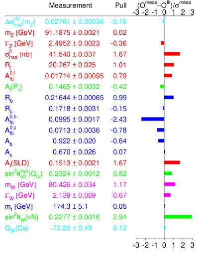
Figure 3: Fits to electroweak data. The bars show the pull from the Standard Model global fit.[3]

The 2-point function of the Z𝑍Z boson is given by,

iΠZZμν=Nc(ig4cW)2(i)2dnk(2π)nTμν[den]𝑖superscriptsubscriptΠ𝑍𝑍𝜇𝜈subscript𝑁𝑐superscript𝑖𝑔4subscript𝑐𝑊2superscript𝑖2superscript𝑑𝑛𝑘superscript2𝜋𝑛superscript𝑇𝜇𝜈delimited-[]𝑑𝑒𝑛i\Pi_{ZZ}^{\mu\nu}=-N_{c}({-ig\over 4c_{W}})^{2}(i)^{2}\int{d^{n}k\over(2\pi)^{n}}{T^{\mu\nu}\over[den]} (13)

where cWcosθWsubscript𝑐𝑊subscript𝜃𝑊c_{W}\equiv\cos\theta_{W} and ,

Tμνsuperscript𝑇𝜇𝜈\displaystyle T^{\mu\nu} =\displaystyle= Tr[(k+Mt)γμ(RtP++LtP)(kp+Mt)γν(RtP++LtP)]𝑇𝑟delimited-[]𝑘subscript𝑀𝑡superscript𝛾𝜇subscript𝑅𝑡subscript𝑃subscript𝐿𝑡subscript𝑃𝑘𝑝subscript𝑀𝑡superscript𝛾𝜈subscript𝑅𝑡subscript𝑃subscript𝐿𝑡subscript𝑃\displaystyle Tr[(k+M_{t})\gamma^{\mu}(R_{t}P_{+}+L_{t}P_{-})(k-p+M_{t})\gamma^{\nu}(R_{t}P_{+}+L_{t}P_{-})]
den𝑑𝑒𝑛\displaystyle den =\displaystyle= [k2Mt2][(k+p)2Mt2],delimited-[]superscript𝑘2superscriptsubscript𝑀𝑡2delimited-[]superscript𝑘𝑝2superscriptsubscript𝑀𝑡2\displaystyle[k^{2}-M_{t}^{2}][(k+p)^{2}-M_{t}^{2}]~{}, (14)

and P±=12(1±γ5)subscript𝑃plus-or-minus12plus-or-minus1subscript𝛾5P_{\pm}={1\over 2}(1\pm\gamma_{5}). The coupling of the Z𝑍Z to the top quark is given in Eq. 5 and p𝑝p is the external gauge boson momentum. Shifting momentum in the integral, kkpxsuperscript𝑘𝑘𝑝𝑥k^{\prime}\rightarrow k-px, and using Feynman parameters, the integral in n=42ϵ𝑛42italic-ϵn=4-2\epsilon dimensions becomes,

iΠZZμν𝑖superscriptsubscriptΠ𝑍𝑍𝜇𝜈\displaystyle i\Pi_{ZZ}^{\mu\nu} =\displaystyle= Nc(ig4cW)2(i)2dnk(2π)n01𝑑xsubscript𝑁𝑐superscript𝑖𝑔4subscript𝑐𝑊2superscript𝑖2superscript𝑑𝑛superscript𝑘superscript2𝜋𝑛subscriptsuperscript10differential-d𝑥\displaystyle-N_{c}({-ig\over 4c_{W}})^{2}(i)^{2}\int{d^{n}k^{\prime}\over(2\pi)^{n}}\int^{1}_{0}dx (15)
[4k2(1+ϵ2)(Rt2+Lt2)+16LtRtMt2]gμν+(k2+p2x(1x)Mt2)2,delimited-[]4superscript𝑘21italic-ϵ2superscriptsubscript𝑅𝑡2superscriptsubscript𝐿𝑡216subscript𝐿𝑡subscript𝑅𝑡superscriptsubscript𝑀𝑡2superscript𝑔𝜇𝜈superscriptsuperscript𝑘2superscript𝑝2𝑥1𝑥superscriptsubscript𝑀𝑡22\displaystyle~{}~{}~{}~{}{[4k^{\prime~{}2}(-1+{\epsilon\over 2})(R_{t}^{2}+L_{t}^{2})+16L_{t}R_{t}M_{t}^{2}]g^{\mu\nu}+...\over(k^{\prime~{}2}+p^{2}x(1-x)-M_{t}^{2})^{2}}~{},

where we retain only those terms contributing to AZZ(0)subscript𝐴𝑍𝑍0A_{ZZ}(0). The result proportional to Mt2superscriptsubscript𝑀𝑡2M_{t}^{2} is,

AZZ(p2=0)=g2Nc32π2cW2(4πMt2)ϵMt2ϵ(RtLt)2.subscript𝐴𝑍𝑍superscript𝑝20superscript𝑔2subscript𝑁𝑐32superscript𝜋2superscriptsubscript𝑐𝑊2superscript4𝜋superscriptsubscript𝑀𝑡2italic-ϵsuperscriptsubscript𝑀𝑡2italic-ϵsuperscriptsubscript𝑅𝑡subscript𝐿𝑡2A_{ZZ}(p^{2}=0)={g^{2}N_{c}\over 32\pi^{2}c_{W}^{2}}\biggl{(}{4\pi\over M_{t}^{2}}\biggr{)}^{\epsilon}{M_{t}^{2}\over\epsilon}(R_{t}-L_{t})^{2}. (16)

The analogous result for the W𝑊W two-point function is,

AWW(p2=0)=g2Nc32π2(4πMt2)ϵMt2(1ϵ+12).subscript𝐴𝑊𝑊superscript𝑝20superscript𝑔2subscript𝑁𝑐32superscript𝜋2superscript4𝜋superscriptsubscript𝑀𝑡2italic-ϵsuperscriptsubscript𝑀𝑡21italic-ϵ12A_{WW}(p^{2}=0)={g^{2}N_{c}\over 32\pi^{2}}\biggl{(}{4\pi\over M_{t}^{2}}\biggr{)}^{\epsilon}M_{t}^{2}\biggl{(}{1\over\epsilon}+{1\over 2}\biggr{)}~{}. (17)

Combining Eqs. 16 and 17, the contribution to the ρ𝜌\rho parameter which is proportional to Mt2superscriptsubscript𝑀𝑡2M_{t}^{2} is found from Eq. 11,[10]

δρ=g2Nc64π2Mt2MW2=GFNcMt282π2.𝛿𝜌superscript𝑔2subscript𝑁𝑐64superscript𝜋2superscriptsubscript𝑀𝑡2superscriptsubscript𝑀𝑊2subscript𝐺𝐹subscript𝑁𝑐superscriptsubscript𝑀𝑡282superscript𝜋2\delta\rho={g^{2}N_{c}\over 64\pi^{2}}{M_{t}^{2}\over M_{W}^{2}}={G_{F}N_{c}M_{t}^{2}\over 8\sqrt{2}\pi^{2}}~{}. (18)

Experimentally[4] ρ=1.00126.0014+.0023𝜌subscriptsuperscript1.00126.0023.0014\rho=1.00126^{+.0023}_{-.0014}[4] and so an upper limit on the top quark mass can be obtained from Eq. 18.

Many of the precision measurements shown in Fig. 3 are sensitive to Mt2superscriptsubscript𝑀𝑡2M_{t}^{2} and so a prediction for the top quark mass can be extracted quite precisely by combining many measurements. In fact, precision measurements were sensitive to the top quark mass before top was discovered at Fermilab!
Refer to caption
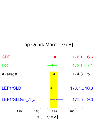
Figure 4: Measurements of the top quark mass at Fermilab (CDF and D0) and indirect predictions from precision measurements (LEP1, SLD and MWsubscript𝑀𝑊M_{W}).[3]

The agreement between the direct measurement of the top quark mass in the Fermilab collider experiments and the indirect prediction from the precision measurements (as shown in Fig. 4) is one of the triumphs of the Standard Model. It is interesting to note that a similar limit on the Higgs boson mass from precision measurements gives Mh<193GeVsubscript𝑀193𝐺𝑒𝑉M_{h}<193~{}GeV at the 95%percent9595\% confidence level.[3] Precision measurements depend logarithmically on the Higgs mass, and so it is much more difficult to bound the Higgs mass in this manner than it is to restrict the top quark mass. Increases in the experimental precisions of the top quark mass and the W𝑊W boson mass in Run II measurements at the Tevatron will provide an improved bound on the Higgs boson mass, δMh/Mh40%.similar-to𝛿subscript𝑀subscript𝑀percent40\delta M_{h}/M_{h}\sim 40\%.[11]

In the next sections, we discuss the discovery of the top quark at Fermilab and the experimental exploration of the top quark properties, both at Fermilab and the LHC and at a future high energy e+esuperscript𝑒superscript𝑒e^{+}e^{-} collider.

3 Top Quark Properties

3.1 Hadronic Production

The top quark was discovered in 1995 at Fermilab in pp¯𝑝¯𝑝p{\overline{p}} collisions at S=1.8TeV𝑆1.8𝑇𝑒𝑉\sqrt{S}=1.8~{}TeV.[1] This data set (called Run I) consists of an integrated luminosity of L125pb1similar-to𝐿125𝑝superscript𝑏1{\it L}\sim 125~{}pb^{-1}. Both CDF and D0 are currently rediscovering the top quark in the Run II data set. Run II will produce roughly 500 clean top quark events for each inverse femtobarn of data and so precision measurements of many top quark properties will be possible.

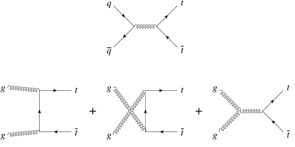
In hadronic interactions, the top quark is produced by gluon fusion and by qq¯𝑞¯𝑞q{\overline{q}} annihilation as shown in Fig. 5,

gg𝑔𝑔\displaystyle gg \displaystyle\rightarrow tt¯𝑡¯𝑡\displaystyle t{\overline{t}}
qq¯𝑞¯𝑞\displaystyle q{\overline{q}} \displaystyle\rightarrow tt¯.𝑡¯𝑡\displaystyle t{\overline{t}}. (19)
Refer to caption

.

Figure 5: Feynman diagrams contributing to top quark pair production in hadron colliders.

The hadronic top quark production cross section, σHsubscript𝜎𝐻\sigma_{H}, at the Tevatron, pp¯tt¯𝑝¯𝑝𝑡¯𝑡p{\overline{p}}\rightarrow t{\overline{t}}, (or pptt¯𝑝𝑝𝑡¯𝑡pp\rightarrow t{\overline{t}} at the LHC) is found by convoluting the parton level cross section with the parton distribution functions (PDFs),

σH(S)=Σijfi(x1,μ)fj(x2,μ)σ^ij(x1x2S,μ),subscript𝜎𝐻𝑆subscriptΣ𝑖𝑗subscript𝑓𝑖subscript𝑥1𝜇subscript𝑓𝑗subscript𝑥2𝜇subscript^𝜎𝑖𝑗subscript𝑥1subscript𝑥2𝑆𝜇\sigma_{H}(S)=\Sigma_{ij}\int f_{i}(x_{1},\mu)f_{j}(x_{2},\mu){\hat{\sigma}}_{ij}(x_{1}x_{2}S,\mu), (20)

where the hadronic center of mass energy is S𝑆S, the partonic center of mass energy is s=x1x2S𝑠subscript𝑥1subscript𝑥2𝑆s=x_{1}x_{2}S, the parton distribution functions are fi(x,μ)subscript𝑓𝑖𝑥𝜇f_{i}(x,\mu), and the parton level cross section is σ^ij(s,μ)subscript^𝜎𝑖𝑗𝑠𝜇{\hat{\sigma}}_{ij}(s,\mu). The parameter μ𝜇\mu is an unphysical renormalization/factorization scale. To O(αs2)𝑂superscriptsubscript𝛼𝑠2{\it O}(\alpha_{s}^{2}), the sum in Eq. 20 is over the qq¯𝑞¯𝑞q{\overline{q}} and gg𝑔𝑔gg initial states shown in Fig. 5.

It is useful to parameterize the parton level cross section (to next-to-leading order in αssubscript𝛼𝑠\alpha_{s}) as,

σ^ij(s,μ)=αs2(μ)Mt2[hij0(ρ)+hij1αs(μ)+hij2αs(μ)log(μ2Mt2)].subscript^𝜎𝑖𝑗𝑠𝜇superscriptsubscript𝛼𝑠2𝜇superscriptsubscript𝑀𝑡2delimited-[]subscriptsuperscript0𝑖𝑗𝜌subscriptsuperscript1𝑖𝑗subscript𝛼𝑠𝜇subscriptsuperscript2𝑖𝑗subscript𝛼𝑠𝜇superscript𝜇2superscriptsubscript𝑀𝑡2{\hat{\sigma}}_{ij}(s,\mu)={\alpha_{s}^{2}(\mu)\over M_{t}^{2}}\biggl{[}h^{0}_{ij}(\rho)+h^{1}_{ij}\alpha_{s}(\mu)+h^{2}_{ij}\alpha_{s}(\mu)\log\biggl{(}{\mu^{2}\over M_{t}^{2}}\biggr{)}\biggr{]}~{}. (21)

At lowest order, O(αs2)𝑂superscriptsubscript𝛼𝑠2{\it O}(\alpha_{s}^{2}), the parton level cross sections are,[12]

hqq¯0subscriptsuperscript0𝑞¯𝑞\displaystyle h^{0}_{q{\overline{q}}} =\displaystyle= πβρ27(2+ρ)𝜋𝛽𝜌272𝜌\displaystyle{\pi\beta\rho\over 27}(2+\rho)
hgg0subscriptsuperscript0𝑔𝑔\displaystyle h^{0}_{gg} =\displaystyle= πβρ192[1β(ρ2+16ρ+16)log(1+β1β)2831ρ]𝜋𝛽𝜌192delimited-[]1𝛽superscript𝜌216𝜌161𝛽1𝛽2831𝜌\displaystyle{\pi\beta\rho\over 192}\biggl{[}{1\over\beta}(\rho^{2}+16\rho+16)\log\biggl{(}{1+\beta\over 1-\beta}\biggr{)}-28-31\rho\biggr{]}
hqg0subscriptsuperscript0𝑞𝑔\displaystyle h^{0}_{qg} =\displaystyle= 0,0\displaystyle 0~{}, (22)

where

ρ𝜌\displaystyle\rho =\displaystyle= 4Mt2s4superscriptsubscript𝑀𝑡2𝑠\displaystyle{4M_{t}^{2}\over s}
β𝛽\displaystyle\beta =\displaystyle= 1ρ.1𝜌\displaystyle\sqrt{1-\rho}~{}. (23)

The threshold condition is ρ=1𝜌1\rho=1 and so σ^ijsubscript^𝜎𝑖𝑗{\hat{\sigma}}_{ij} vanishes at threshold.

To any given order in αs(μ)subscript𝛼𝑠𝜇\alpha_{s}(\mu), the hadronic cross section σHsubscript𝜎𝐻\sigma_{H} must be independent of μ𝜇\mu,

dσHdlogμ2=0.𝑑subscript𝜎𝐻𝑑superscript𝜇20{d\sigma_{H}\over d\log\mu^{2}}=0. (24)

Applying this restriction to Eq. 21 yields,

00\displaystyle 0 =\displaystyle= {f(x1,μ)logμ2f(x2,μ)+f(x1,μ)f(x2,μ)logμ2}σ^(x1x2S,μ)𝑑x1𝑑x2𝑓subscript𝑥1𝜇superscript𝜇2𝑓subscript𝑥2𝜇𝑓subscript𝑥1𝜇𝑓subscript𝑥2𝜇superscript𝜇2^𝜎subscript𝑥1subscript𝑥2𝑆𝜇differential-dsubscript𝑥1differential-dsubscript𝑥2\displaystyle\int\biggl{\{}{\partial f(x_{1},\mu)\over\partial\log\mu^{2}}f(x_{2},\mu)+f(x_{1},\mu){\partial f(x_{2},\mu)\over\partial\log\mu^{2}}\biggr{\}}{\hat{\sigma}}(x_{1}x_{2}S,\mu)dx_{1}dx_{2} (25)
+f(x1,μ)f(x2,μ)σ^(x1x2S,μ)logμ2𝑑x1𝑑x2.𝑓subscript𝑥1𝜇𝑓subscript𝑥2𝜇^𝜎subscript𝑥1subscript𝑥2𝑆𝜇superscript𝜇2differential-dsubscript𝑥1differential-dsubscript𝑥2\displaystyle+\int f(x_{1},\mu)f(x_{2},\mu){\partial{\hat{\sigma}}(x_{1}x_{2}S,\mu)\over\partial\log\mu^{2}}dx_{1}dx_{2}~{}.

The scale dependence of the PDFs is governed by the Altarelli-Parisi evolution functions, Pij(z)subscript𝑃𝑖𝑗𝑧P_{ij}(z):

fi(x,μ)logμ2=αs2πΣjx1dyyPij(xy)fj(y,μ).subscript𝑓𝑖𝑥𝜇superscript𝜇2subscript𝛼𝑠2𝜋subscriptΣ𝑗superscriptsubscript𝑥1𝑑𝑦𝑦subscript𝑃𝑖𝑗𝑥𝑦subscript𝑓𝑗𝑦𝜇{\partial f_{i}(x,\mu)\over\partial\log\mu^{2}}={\alpha_{s}\over 2\pi}\Sigma_{j}\int_{x}^{1}{dy\over y}P_{ij}\biggl{(}{x\over y}\biggr{)}f_{j}(y,\mu)~{}. (26)

Similarly, the scale dependence of the strong coupling constant, αs(μ)subscript𝛼𝑠𝜇\alpha_{s}(\mu), is governed by the evolution of the QCD β𝛽\beta function.

αs(μ)logμ2=b0αs2,subscript𝛼𝑠𝜇superscript𝜇2subscript𝑏0superscriptsubscript𝛼𝑠2{\partial\alpha_{s}(\mu)\over\partial\log\mu^{2}}=-b_{0}\alpha_{s}^{2}\quad, (27)

where b0=(332nlf)12πsubscript𝑏0332subscript𝑛𝑙𝑓12𝜋b_{0}={(33-2n_{lf})\over 12\pi}, and nlfsubscript𝑛𝑙𝑓n_{lf} is the number of light flavors. At next-to-leading order the scale dependence of the various terms must cancel, yielding a prediction for hij2superscriptsubscript𝑖𝑗2h_{ij}^{2},

hij2superscriptsubscript𝑖𝑗2\displaystyle h_{ij}^{2} =\displaystyle= 12π[4πb0hij0(ρ)Σkρ1dzhkj0(ρz)Pki(z)\displaystyle{1\over 2\pi}\biggl{[}4\pi b_{0}h_{ij}^{0}(\rho)-\Sigma_{k}\int_{\rho}^{1}dzh^{0}_{kj}\biggl{(}{\rho\over z}\biggr{)}P_{ki}(z)
Σkρ1dzhik0(ρz)Pkj(z)].\displaystyle-\Sigma_{k}\int_{\rho}^{1}dzh^{0}_{ik}\biggl{(}{\rho\over z}\biggr{)}P_{kj}(z)\biggr{]}.

Using the explicit forms of the Altarelli-Parisi evolution functions, combined with Eq. 22, we find[12]

hqq¯2superscriptsubscript𝑞¯𝑞2\displaystyle h_{q{\overline{q}}}^{2} =\displaystyle= 12π[16πρ81log(1+β1β)+19hqq¯0(ρ)(1276nlf+48log(ρ4β2))]12𝜋delimited-[]16𝜋𝜌811𝛽1𝛽19superscriptsubscript𝑞¯𝑞0𝜌1276subscript𝑛𝑙𝑓48𝜌4superscript𝛽2\displaystyle{1\over 2\pi}\biggl{[}{16\pi\rho\over 81}\log\biggl{(}{1+\beta\over 1-\beta}\biggr{)}+{1\over 9}h_{q{\overline{q}}}^{0}(\rho)\biggl{(}127-6n_{lf}+48\log\biggl{(}{\rho\over 4\beta^{2}}\biggr{)}\biggr{)}\biggr{]}
hgg2superscriptsubscript𝑔𝑔2\displaystyle h_{gg}^{2} =\displaystyle= 12π[π192{2ρ(59ρ2+198ρ288)log(1+β1β)\displaystyle{1\over 2\pi}\biggl{[}{\pi\over 192}\biggl{\{}2\rho\biggl{(}59\rho^{2}+198\rho-288\biggr{)}\log\biggl{(}{1+\beta\over 1-\beta}\biggr{)}
+12ρ(ρ2+16ρ+16)g2(β)6ρ(ρ216ρ+32)g1(β)12𝜌superscript𝜌216𝜌16subscript𝑔2𝛽6𝜌superscript𝜌216𝜌32subscript𝑔1𝛽\displaystyle+12\rho\biggl{(}\rho^{2}+16\rho+16\biggr{)}g_{2}(\beta)-6\rho\biggl{(}\rho^{2}-16\rho+32\biggr{)}g_{1}(\beta)
415β(7449ρ23328ρ+724)}12hgg0(ρ)log(ρ4β2)]\displaystyle-{4\over 15}\beta\biggl{(}7449\rho^{2}-3328\rho+724\biggr{)}\biggr{\}}-12h_{gg}^{0}(\rho)\log\biggl{(}{\rho\over 4\beta^{2}}\biggr{)}\biggr{]}
hqg2superscriptsubscript𝑞𝑔2\displaystyle h_{qg}^{2} =\displaystyle= 1384[4ρ9(14ρ2+27ρ136)log(1+β1β)323ρ(2ρ)g1(β)\displaystyle{1\over 384}\biggl{[}{4\rho\over 9}\biggl{(}14\rho^{2}+27\rho-136\biggr{)}\log\biggl{(}{1+\beta\over 1-\beta}\biggr{)}-{32\over 3}\rho(2-\rho)g_{1}(\beta) (29)
8β135(1319ρ23468ρ+724)]\displaystyle-{8\beta\over 135}\biggl{(}1319\rho^{2}-3468\rho+724\biggr{)}\biggr{]}

where we have defined,

g1(β)subscript𝑔1𝛽\displaystyle g_{1}(\beta) =\displaystyle= log2(1+β2)log2(1β2)+2Li2(1+β2)2Li2(1β2)superscript21𝛽2superscript21𝛽22𝐿subscript𝑖21𝛽22𝐿subscript𝑖21𝛽2\displaystyle\log^{2}\biggl{(}{1+\beta\over 2}\biggr{)}-\log^{2}\biggl{(}{1-\beta\over 2}\biggr{)}+2Li_{2}\biggl{(}{1+\beta\over 2}\biggr{)}-2Li_{2}\biggl{(}{1-\beta\over 2}\biggr{)}
g2(β)subscript𝑔2𝛽\displaystyle g_{2}(\beta) =\displaystyle= Li2(2β1+β)Li2(2β1β).𝐿subscript𝑖22𝛽1𝛽𝐿subscript𝑖22𝛽1𝛽\displaystyle Li_{2}\biggl{(}{2\beta\over 1+\beta}\biggr{)}-Li_{2}\biggl{(}{-2\beta\over 1-\beta}\biggr{)}~{}. (30)

The quantities hij1superscriptsubscript𝑖𝑗1h_{ij}^{1} can only be obtained by performing a complete next-to-leading order calculation[12, 13] and analytic results are not available, although a numerical parameterization is quite accurate. The strong coupling evaluated at the top quark mass is small, αs(Mt)0.1similar-tosubscript𝛼𝑠subscript𝑀𝑡0.1\alpha_{s}(M_{t})\sim 0.1 , and so a perturbative expansion converges rapidly. At energy scales significantly different from the top quark mass, there are also large logarithms of the form (αslog(Mt2Q2))nsuperscriptsubscript𝛼𝑠superscriptsubscript𝑀𝑡2superscript𝑄2𝑛(\alpha_{s}\log({M_{t}^{2}\over Q^{2}}))^{n}, which can be summed to all orders to obtain an improved prediction for the cross section.[14] The inclusion of next-to-leading-logarithm effects reduces the scale dependence of the cross section to roughly ±5%plus-or-minuspercent5\pm 5\%.[15]

Fig. 6 shows the Run I CDF and D0 measured top production cross sections and top quark mass compared with two theoretical predictions. The Run I tt¯𝑡¯𝑡t{\overline{t}} cross sections are,[16]

σtt¯=subscript𝜎𝑡¯𝑡absent\displaystyle\sigma_{t{\overline{t}}}= 6.51.4+1.7pbsubscriptsuperscript6.51.71.4𝑝𝑏\displaystyle 6.5^{+1.7}_{-1.4}~{}pb~{}~{}~{}~{} CDF𝐶𝐷𝐹\displaystyle CDF
σtt¯=subscript𝜎𝑡¯𝑡absent\displaystyle\sigma_{t{\overline{t}}}= 5.9±1.7pbplus-or-minus5.91.7𝑝𝑏\displaystyle 5.9\pm{1.7}~{}pb~{}~{}~{}~{} D0.𝐷0\displaystyle D0~{}. (31)

The curves labelled NLO+NLL include some of the logarithms of the form (αslog(Mt2Q2))nsuperscriptsubscript𝛼𝑠superscriptsubscript𝑀𝑡2superscript𝑄2𝑛(\alpha_{s}\log({M_{t}^{2}\over Q^{2}}))^{n} and the agreement with the experimental results is clearly improved from the NLO prediction alone. An updated theoretical study including next-to-leading-logarithm resummation gives the prediction

σtt¯(S=1.8TeV)=(4.815.29)pbforMt=175GeV,subscript𝜎𝑡¯𝑡𝑆1.8𝑇𝑒𝑉4.815.29𝑝𝑏forsubscript𝑀𝑡175𝐺𝑒𝑉\sigma_{t{\overline{t}}}(\sqrt{S}=1.8~{}TeV)=(4.81-5.29)~{}pb~{}{\hbox{for}}~{}M_{t}=175~{}GeV, (32)

with the range in the prediction corresponding to Mt/2<μ<2Mtsubscript𝑀𝑡2𝜇2subscript𝑀𝑡M_{t}/2<\mu<2M_{t}.[15] The agreement between the predicted and the experimental production rates implies that the top quark is a color triplet, since that rate would be significantly different for a different color representation.

Refer to caption
Figure 6: Fermilab Tevatron Run I cross sections for pp¯tt¯𝑝¯𝑝𝑡¯𝑡p{\overline{p}}\rightarrow t{\overline{t}}. The dashed line is the NLO prediction, while the solid lines incorporate the next-to-leading logarithms.[14]

At the LHC, the subprocess ggtt¯𝑔𝑔𝑡¯𝑡gg\rightarrow t{\overline{t}} dominates the production rate with 90%percent9090\% of the total rate and the cross section is large, σLHC800pbsimilar-tosubscript𝜎𝐿𝐻𝐶800𝑝𝑏\sigma_{LHC}\sim 800~{}pb, yielding about 108superscript10810^{8} tt¯𝑡¯𝑡t{\overline{t}} pairs/year. Because of the large rate, the LHC can search for new physics in top interactions. The large rate also has the implication that top production is often largest background to other new physics signals. A detailed understanding of the top quark signal is therefore a necessary ingredient of new physics searches.

3.2 Weak Interactions of Top

The weak interaction eigenstates are not mass eigenstates,

L=g22Σq=d,s,bt¯γμ(1γ5)VtqqWμ++h.c.𝐿𝑔22subscriptΣ𝑞𝑑𝑠𝑏¯𝑡superscript𝛾𝜇1subscript𝛾5subscript𝑉𝑡𝑞𝑞superscriptsubscript𝑊𝜇h.c.{\it L}=-{g\over 2\sqrt{2}}\Sigma_{q=d,s,b}{\overline{t}}\gamma^{\mu}(1-\gamma_{5})V_{tq}qW_{\mu}^{+}+{\hbox{h.c.}} (33)

and so the interaction of the top quark with a W𝑊W boson and a light quark is proportional to the CKM mixing element, Vtqsubscript𝑉𝑡𝑞V_{tq}. Measurements of the decay rates of the top quark into the lighter quarks therefore translate directly into measurements of the CKM mixing angles.

The unitarity of the CKM matrix and the restriction to 3 generations of fermions gives a limit on Vtbsubscript𝑉𝑡𝑏V_{tb} from the measured values of Vubdelimited-∣∣subscript𝑉𝑢𝑏\mid V_{ub}\mid and Vcbdelimited-∣∣subscript𝑉𝑐𝑏\mid V_{cb}\mid:[4]

1=Vub2+Vcb2+Vtb21superscriptdelimited-∣∣subscript𝑉𝑢𝑏2superscriptdelimited-∣∣subscript𝑉𝑐𝑏2superscriptdelimited-∣∣subscript𝑉𝑡𝑏21=\mid V_{ub}\mid^{2}+\mid V_{cb}\mid^{2}+\mid V_{tb}\mid^{2} (34)

giving,

0.9991<Vtb<0.9994.0.9991delimited-∣∣subscript𝑉𝑡𝑏0.99940.9991<\mid V_{tb}\mid<0.9994~{}. (35)

If there are more than 3 generations, however, Eq. 34 is no longer valid and there is almost no limit from unitarity on Vtbsubscript𝑉𝑡𝑏V_{tb}.

Unitarity in the three generation model can be tested by measuring the ratio of the rate for top decays to the b𝑏b quark to the rate for top decays to lighter quarks,[17]

RtbΓ(tWb)Γ(tWq)subscript𝑅𝑡𝑏Γ𝑡𝑊𝑏Γ𝑡𝑊𝑞\displaystyle R_{tb}\equiv{\Gamma(t\rightarrow Wb)\over\Gamma(t\rightarrow Wq)} =\displaystyle= Vtb2Vtd2+Vts2+Vtb2superscriptdelimited-∣∣subscript𝑉𝑡𝑏2superscriptdelimited-∣∣subscript𝑉𝑡𝑑2superscriptdelimited-∣∣subscript𝑉𝑡𝑠2superscriptdelimited-∣∣subscript𝑉𝑡𝑏2\displaystyle{\mid V_{tb}\mid^{2}\over\mid V_{td}\mid^{2}+\mid V_{ts}\mid^{2}+\mid V_{tb}\mid^{2}} (36)
=\displaystyle= .94.24+.31(CDF)subscriptsuperscript.94.31.24𝐶𝐷𝐹\displaystyle.94^{+.31}_{-.24}~{}~{}~{}(CDF)

This quantity can be measured at Fermilab by counting the number of tagged b𝑏b’s in a top quark event. Since the b𝑏b quark lives approximately 1.5ps1.5𝑝𝑠1.5~{}ps, the b𝑏b quark will travel 450μm450𝜇𝑚450~{}\mu m before decaying. The secondary b𝑏b vertex can then be measured with a silicon vertex detector. Assuming unitarity of the CKM matrix, the denominator of Eq. 36 is 111, and the measurement can be interpreted as a measurement of Vtbsubscript𝑉𝑡𝑏V_{tb},

Vtb=.97.12+.15,delimited-∣∣subscript𝑉𝑡𝑏subscriptsuperscript.97.15.12\mid V_{tb}\mid=.97^{+.15}_{-.12}, (37)

consistent with Eq. 35.

If there is a fourth generation of quarks, (t,b)superscript𝑡superscript𝑏(t^{\prime},b^{\prime}), the charge 1313-{1\over 3} bsuperscript𝑏b^{\prime} is experimentally restricted to be heavier than mtMWsubscript𝑚𝑡subscript𝑀𝑊m_{t}-M_{W},[4] and so the top quark cannot decay into the bsuperscript𝑏b^{\prime}. Then the denominator of Rtbsubscript𝑅𝑡𝑏R_{tb} need not equal 111, and the measurement implies only Vtb>>Vts,Vtdmuch-greater-thandelimited-∣∣subscript𝑉𝑡𝑏delimited-∣∣subscript𝑉𝑡𝑠delimited-∣∣subscript𝑉𝑡𝑑\mid V_{tb}\mid>>\mid V_{ts}\mid,~{}\mid V_{td}\mid.

The direct measurement of Vtdsubscript𝑉𝑡𝑑V_{td} in single top production will be discussed in Section 3.6.

Refer to caption
Figure 7: Feynman diagram for top decay to Wb𝑊𝑏Wb.

3.3 Top Quark Decay

The top quark is the only quark which decays before it can form a bound state. This is due to the very short lifetime of the top quark,

τt5×1025sec,similar-tosubscript𝜏𝑡5superscript1025𝑠𝑒𝑐\tau_{t}\sim 5\times 10^{-25}~{}sec~{}, (38)

compared to the QCD time scale:

τQCD3×1024sec.similar-tosubscript𝜏𝑄𝐶𝐷3superscript1024𝑠𝑒𝑐\tau_{QCD}\sim 3\times 10^{-24}~{}sec~{}. (39)

This is very different from the b𝑏b quark system, where the b𝑏b quark combines with the lighter quarks to form B𝐵B mesons, which then decay.

Since Vtb1similar-todelimited-∣∣subscript𝑉𝑡𝑏1\mid V_{tb}\mid\sim 1, the dominant decay of the top quark is

t(p)Wμ(pW)+b(p),𝑡𝑝superscript𝑊𝜇subscript𝑝𝑊𝑏superscript𝑝t(p)\rightarrow W^{\mu}(p_{W})+b(p^{\prime}), (40)

The lowest order amplitude is shown in Fig. 7 and is,

A0(tWμb)=g22u¯(p)γμ(1γ5)u(p).subscript𝐴0𝑡superscript𝑊𝜇𝑏𝑔22¯𝑢superscript𝑝superscript𝛾𝜇1subscript𝛾5𝑢𝑝{\it A}_{0}(t\rightarrow W^{\mu}b)=-{g\over 2\sqrt{2}}{\overline{u}}(p^{\prime})\gamma^{\mu}(1-\gamma_{5})u(p)~{}. (41)

Squaring the amplitude, and summing over the W𝑊W polarization vectors,

Σϵμ(pW)ϵν(pW)=gμν+pWμpWνMW2,Σsuperscriptitalic-ϵ𝜇subscript𝑝𝑊superscriptitalic-ϵabsent𝜈subscript𝑝𝑊superscript𝑔𝜇𝜈superscriptsubscript𝑝𝑊𝜇superscriptsubscript𝑝𝑊𝜈superscriptsubscript𝑀𝑊2\Sigma\epsilon^{\mu}(p_{W})\epsilon^{*\nu}(p_{W})=-g^{\mu\nu}+{p_{W}^{\mu}p_{W}^{\nu}\over M_{W}^{2}}, (42)

gives the amplitude-squared,

A0(tWb)2=g2(Mt2MW2)[1+Mt22MW2].superscriptdelimited-∣∣subscript𝐴0𝑡𝑊𝑏2superscript𝑔2superscriptsubscript𝑀𝑡2superscriptsubscript𝑀𝑊2delimited-[]1superscriptsubscript𝑀𝑡22superscriptsubscript𝑀𝑊2\mid{\it A}_{0}(t\rightarrow Wb)\mid^{2}=g^{2}(M_{t}^{2}-M_{W}^{2})\biggl{[}1+{M_{t}^{2}\over 2M_{W}^{2}}\biggr{]}~{}. (43)

The total decay width is

Γ0(tWb)=(12)12MtA0(tWb)2(dPS2).subscriptΓ0𝑡𝑊𝑏1212subscript𝑀𝑡superscriptdelimited-∣∣subscript𝐴0𝑡𝑊𝑏2𝑑𝑃subscript𝑆2\Gamma_{0}(t\rightarrow Wb)=\biggl{(}{1\over 2}\biggr{)}{1\over 2M_{t}}\int\mid{\it A}_{0}(t\rightarrow Wb)\mid^{2}(dPS_{2})~{}. (44)

The factor of 1212{1\over 2} is the average over the initial top quark spin, and the phase space factor is,

(dPS2)=Mt2MW28πMt2.𝑑𝑃subscript𝑆2superscriptsubscript𝑀𝑡2superscriptsubscript𝑀𝑊28𝜋superscriptsubscript𝑀𝑡2(dPS_{2})={M_{t}^{2}-M_{W}^{2}\over 8\pi M_{t}^{2}}~{}. (45)

Including the CKM mixing, the final result is then,

Γ0(tbW+)Vtb2GFMt38π2(1MW2Mt2)2(1+2MW2Mt2).similar-tosubscriptΓ0𝑡𝑏superscript𝑊superscriptdelimited-∣∣subscript𝑉𝑡𝑏2subscript𝐺𝐹superscriptsubscript𝑀𝑡38𝜋2superscript1superscriptsubscript𝑀𝑊2superscriptsubscript𝑀𝑡2212superscriptsubscript𝑀𝑊2superscriptsubscript𝑀𝑡2\Gamma_{0}(t\rightarrow bW^{+})\sim\mid V_{tb}\mid^{2}{G_{F}M_{t}^{3}\over 8\pi\sqrt{2}}\biggl{(}1-{M_{W}^{2}\over M_{t}^{2}}\biggr{)}^{2}\biggl{(}1+{2M_{W}^{2}\over M_{t}^{2}}\biggr{)}. (46)

Higher order QCD corrections can be calculated in a straightforward manner and yield a precise prediction for the decay width,[9, 18]

Γ(tbW+)=Vtb21.42GeV.Γ𝑡𝑏superscript𝑊superscriptdelimited-∣∣subscript𝑉𝑡𝑏21.42𝐺𝑒𝑉\Gamma(t\rightarrow bW^{+})=\mid V_{tb}\mid^{2}1.42~{}GeV.

3.4 W𝑊W Helicity in Top Quark Decay

The helicity structure of the top quark decays is interesting because it yields information on the VA𝑉𝐴V-A nature of the tbW𝑡𝑏𝑊tbW vertex as is clear from Eq. 41. The top quark is produced through the weak interactions as a left-handed fermion (neglecting the b𝑏b quark mass), which has spin opposite from the direction of the top quark motion.

If the W𝑊W is produced as a longitudinal W𝑊W (helicity 00), then its momentum and polarization vectors are (see Fig. 8):

Refer to caption
Figure 8: Spin vectors for longitudinally polarized W𝑊W’s produced in the decay tWb𝑡𝑊𝑏t\rightarrow Wb.
pWsubscript𝑝𝑊\displaystyle p_{W} =\displaystyle= (EW,0,0,pW)subscript𝐸𝑊00delimited-∣∣subscript𝑝𝑊\displaystyle(E_{W},0,0,\mid{\vec{p}_{W}}\mid)
ϵLWsuperscriptsubscriptitalic-ϵ𝐿𝑊\displaystyle\epsilon_{L}^{W} =\displaystyle= 1MW(pW,0,0,EW)1subscript𝑀𝑊delimited-∣∣subscript𝑝𝑊00subscript𝐸𝑊\displaystyle{1\over M_{W}}(\mid{\vec{p}_{W}}\mid,0,0,E_{W}) (47)
similar-to\displaystyle\sim pWMW+O(MWMt).delimited-∣∣subscript𝑝𝑊subscript𝑀𝑊𝑂subscript𝑀𝑊subscript𝑀𝑡\displaystyle{\mid{\vec{p}_{W}}\mid\over M_{W}}+{\it O}\biggl{(}{M_{W}\over M_{t}}\biggr{)}~{}.

The amplitude for a top decaying into a longitudinal W𝑊W is then,

A(tbWL)𝐴𝑡𝑏subscript𝑊𝐿\displaystyle{\it A}(t\rightarrow bW_{L}) =\displaystyle= g22b¯pWMW(1γ5)t+O(MWMt)𝑔22¯𝑏subscript𝑝𝑊subscript𝑀𝑊1subscript𝛾5𝑡𝑂subscript𝑀𝑊subscript𝑀𝑡\displaystyle-{g\over 2\sqrt{2}}{\overline{b}}{p_{W}\over M_{W}}(1-\gamma_{5})t+{\it O}\biggl{(}{M_{W}\over M_{t}}\biggr{)} (48)
=\displaystyle= mt2vb¯(1+γ5)t+O(MWMt).subscript𝑚𝑡2𝑣¯𝑏1subscript𝛾5𝑡𝑂subscript𝑀𝑊subscript𝑀𝑡\displaystyle-{m_{t}\over\sqrt{2}v}{\overline{b}}(1+\gamma_{5})t+{\it O}\biggl{(}{M_{W}\over M_{t}}\biggr{)}~{}.

This gives the result that the decay of the top into longitudinal W𝑊W’s is,

Γ(tbWL)mt3v2.similar-toΓ𝑡𝑏subscript𝑊𝐿superscriptsubscript𝑚𝑡3superscript𝑣2\Gamma(t\rightarrow bW_{L})\sim{m_{t}^{3}\over v^{2}}~{}. (49)

The decay of the top quark into a positive helicity W𝑊W, hW=+superscript𝑊h^{W}=+, is forbidden by angular momentum conservation since a massless b𝑏b quark is always left-handed, while the heavy top can be either left- or right-handed. This is illustrated in Fig. 9. CDF has measured the decay of the top quark to a right handed W𝑊W and finds a result consistent with 00,[19]

BR(tbWR)=.11±0.15.𝐵𝑅𝑡𝑏subscript𝑊𝑅plus-or-minus.110.15BR(t\rightarrow bW_{R})=.11\pm 0.15~{}. (50)
Refer to caption
Figure 9: Spin vectors for positive helicity (right handed) W𝑊W’s produced in the decay tWb𝑡𝑊𝑏t\rightarrow Wb. Conservation of angular momentum forbids this decay.
Refer to caption
Figure 10: Spin vectors for transverse helicity W𝑊W’s produced in the decay tWb𝑡𝑊𝑏t\rightarrow Wb.

For a transversely polarized W𝑊W, the polarization vector is given by,

ϵ±W=12(0,1,±i,0).superscriptsubscriptitalic-ϵplus-or-minus𝑊1201plus-or-minus𝑖0\epsilon_{\pm}^{W}={1\over\sqrt{2}}(0,1,\pm i,0)~{}. (51)

This gives a decay rate,

Γ(tbWT)g2mt.similar-toΓ𝑡𝑏subscript𝑊𝑇superscript𝑔2subscript𝑚𝑡\Gamma(t\rightarrow bW_{T})\sim g^{2}m_{t}~{}. (52)

Comparing Eqs. 49 and 52, it is clear that the rate for top decay to transverse W𝑊W’s is suppressed relative to that for decay to longitudinal W𝑊W’s,

F0subscript𝐹0\displaystyle{\it F}_{0} =\displaystyle= Γ(tbWL)Γ(tWb)TOTΓ𝑡𝑏subscript𝑊𝐿Γsubscript𝑡𝑊𝑏𝑇𝑂𝑇\displaystyle{\Gamma(t\rightarrow bW_{L})\over\Gamma(t\rightarrow Wb)_{TOT}} (53)
=\displaystyle= mt22MW21+mt22MW2superscriptsubscript𝑚𝑡22superscriptsubscript𝑀𝑊21superscriptsubscript𝑚𝑡22superscriptsubscript𝑀𝑊2\displaystyle{{m_{t}^{2}\over 2M_{W}^{2}}\over 1+{m_{t}^{2}\over 2M_{W}^{2}}}
=\displaystyle= 70.1%.percent70.1\displaystyle 70.1\%~{}.

Can we measure this? The W𝑊W helicity is correlated with the momentum of the decay leptons: hW=+superscript𝑊h^{W}=+ gives harder charged leptons than hW=superscript𝑊h^{W}=-. A preliminary measurement of the polarization of the W𝑊W’s in top decay yields,[19]

F0=91±37±13%CDF,subscript𝐹0plus-or-minus9137percent13𝐶𝐷𝐹{\it F}_{0}=91\pm 37\pm 13\%~{}~{}CDF, (54)

consistent with Eq. 53. With 2fb12𝑓superscript𝑏12~{}fb^{-1} of data from Run II at the Tevatron, a more definitive (5%similar-toabsentpercent5\sim 5\%) measurement of F0subscript𝐹0{\it F}_{0} will be possible.[20]

3.5 Top Production and Decay

The Tevatron and the LHC produce predominantly tt¯𝑡¯𝑡t{\overline{t}} pairs, which decay almost entirely by tWb𝑡𝑊𝑏t\rightarrow Wb (since Vtb1similar-todelimited-∣∣subscript𝑉𝑡𝑏1\mid V_{tb}\mid\sim 1),222Recent reviews of the experimental issues involved in top quark physics can be found in Ref. \refciteworm.

pp¯tt¯W+Wbb¯.𝑝¯𝑝𝑡¯𝑡superscript𝑊superscript𝑊𝑏¯𝑏p{\overline{p}}\rightarrow t{\overline{t}}\rightarrow W^{+}W^{-}b{\overline{b}}. (55)

It is useful to classify top quark events by the decay pattern of the W+Wsuperscript𝑊superscript𝑊W^{+}W^{-} pair:

  • Di-lepton: Roughly 5%percent55\% of the tt¯𝑡¯𝑡t{\overline{t}} events fall into this category,

    W+superscript𝑊\displaystyle W^{+} \displaystyle\rightarrow l+ν,l=e,μformulae-sequencesuperscript𝑙𝜈𝑙𝑒𝜇\displaystyle l^{+}\nu,~{}~{}l=e,\mu
    Wsuperscript𝑊\displaystyle W^{-} \displaystyle\rightarrow lν.superscript𝑙𝜈\displaystyle l^{-}\nu~{}. (56)

    Since Br(Weν)+BR(Wμν)22%similar-to𝐵𝑟𝑊𝑒𝜈𝐵𝑅𝑊𝜇𝜈percent22Br(W\rightarrow e\nu)+BR(W\rightarrow\mu\nu)\sim 22\%, the 125pb1125𝑝superscript𝑏1125~{}pb^{-1} at Run I of the Tevatron produced 625similar-toabsent625\sim 625 tt¯𝑡¯𝑡t{\overline{t}} events which yielded .22×.22×62530similar-toabsent.22.22625similar-to30\sim.22\times.22\times 625\sim 30 di-lepton events. These events are clean, but suffer from the small statistics.

  • lepton + jets: This class of events comprises roughly 30%percent3030\% of the total,

    W±l±ν,Wjets.formulae-sequencesuperscript𝑊plus-or-minussuperscript𝑙plus-or-minus𝜈superscript𝑊minus-or-plus𝑗𝑒𝑡𝑠W^{\pm}\rightarrow l^{\pm}\nu,~{}~{}W^{\mp}\rightarrow jets~{}. (57)

    Lepton plus jet events are fully reconstructable and have small backgrounds. Assuming at least 1 b𝑏b quark is tagged, CDF observed 34 such events in Run I, with an expected background of 8.[22] In Run II, with 2fb12𝑓superscript𝑏12~{}fb^{-1}, there should be 1000 lepton+jets events/experiment. This increase from Run I results from higher luminosity, the higher cross section at S=2TeV𝑆2𝑇𝑒𝑉\sqrt{S}=2~{}TeV compared to S=1.8TeV𝑆1.8𝑇𝑒𝑉\sqrt{S}=1.8~{}TeV, and upgraded detectors with improved capabilities for b𝑏b-tagging.

    This channel produced the most precise measurement of the cross section for top pair production. The combined average from CDF and D0 at Run I is,

    σ(pp¯tt¯)S=1.8TeV=5.9±1.7pbevaluated-at𝜎𝑝¯𝑝𝑡¯𝑡𝑆1.8𝑇𝑒𝑉plus-or-minus5.91.7𝑝𝑏\sigma(p{\overline{p}}\rightarrow t{\overline{t}})\mid_{\sqrt{S}=1.8~{}TeV}=5.9\pm 1.7~{}pb (58)
  • All jets: 44%percent4444\% of the events fall into this category. This class of events was observed by both CDF/D0 at Run I, with large backgrounds.

3.6 Single Top Production

Single top production can provide a precise measurement of Vtbsubscript𝑉𝑡𝑏V_{tb}. The dominant production processes at the Tevatron are the t𝑡t channel W𝑊W exchange and the s𝑠s channel qq¯𝑞¯𝑞q{\overline{q}} annihilation shown in Fig. 11. At the LHC, the subprocess gbtW𝑔𝑏𝑡𝑊gb\rightarrow tW is also important. The contributions (to NLO QCD) of the various subprocesses at the Tevatron and the LHC are given in Table 2.[23, 24] All of these processes are proportional to Vtb2superscriptdelimited-∣∣subscript𝑉𝑡𝑏2\mid V_{tb}\mid^{2}.

\tbl

Contributions to single top production at the Tevatron and the LHC. Tevatron, RunII LHC σqbsubscript𝜎𝑞𝑏\sigma_{qb} 2.1pb2.1𝑝𝑏2.1~{}pb 238pb238𝑝𝑏238~{}pb σqq¯subscript𝜎𝑞¯𝑞\sigma_{q{\overline{q}}} .9pb.9𝑝𝑏.9~{}pb 10pb10𝑝𝑏10~{}pb σgbsubscript𝜎𝑔𝑏\sigma_{gb} .1pb.1𝑝𝑏.1~{}pb 56pb56𝑝𝑏56~{}pb

Refer to caption
Figure 11: Feynman diagrams contributing to single top production at the Tevatron and the LHC.

Single top production was not observed in Run I, and both experiments set limits on the production rate. At Run II of the Tevatron, and at the LHC, single top production can be observed with a rate roughly half that of the tt¯𝑡¯𝑡t{\overline{t}} rate and will lead to a measurement at the Tevatron of,

δVtbVtb5%similar-todelimited-∣∣𝛿subscript𝑉𝑡𝑏subscript𝑉𝑡𝑏percent5\mid{\delta V_{tb}\over V_{tb}}\mid\sim 5\%

with 30fb130𝑓superscript𝑏130~{}fb^{-1} of data. With 2fb12𝑓superscript𝑏12~{}fb^{-1}, the Tevatron Run II should achieve an accuracy of δVtbVtb13%similar-todelimited-∣∣𝛿subscript𝑉𝑡𝑏subscript𝑉𝑡𝑏percent13\mid{\delta V_{tb}\over V_{tb}}\mid\sim 13\%.[20]

3.7 Measurements of Mtsubscript𝑀𝑡M_{t}

Mtsubscript𝑀𝑡M_{t} is a fundamental parameter of the Standard Model, but the value is not predicted (except indirectly from precision measurements such as the ρ𝜌\rho parameter discussed earlier). In the Standard Model, a precise value of Mtsubscript𝑀𝑡M_{t} is important primarily for its role in precision electroweak observables and for the prediction for the Higgs boson mass extracted from these measurements.[25] In extentions of the Standard Model, such as those discussed in Section 5, a precise knowledge of Mtsubscript𝑀𝑡M_{t} plays a critical role in defining the parameters of the theory.
Refer to caption
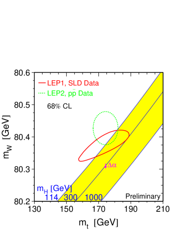
Figure 12: Implications of precision measurements of Mtsubscript𝑀𝑡M_{t} and MWsubscript𝑀𝑊M_{W} on the indirect extraction of the Higgs boson mass. The Standard Model allows only the shaded region.[3]

The top quark mass was measured in Run I at the Tevatron and the most accurate value of Mtsubscript𝑀𝑡M_{t} comes from the single lepton+jets channel,[2]

Mtsubscript𝑀𝑡\displaystyle M_{t} =\displaystyle= 176.1±4.8(stat)±5.3(syst)CDFplus-or-minus176.14.8𝑠𝑡𝑎𝑡5.3𝑠𝑦𝑠𝑡𝐶𝐷𝐹\displaystyle 176.1\pm 4.8~{}(stat)\pm 5.3~{}(syst)~{}~{}~{}CDF (59)
=\displaystyle= 173.3±5.6(stat)±5.5(syst)D0.plus-or-minus173.35.6𝑠𝑡𝑎𝑡5.5𝑠𝑦𝑠𝑡𝐷0\displaystyle 173.3\pm 5.6~{}(stat)\pm 5.5~{}(syst)~{}~{}~{}D0~{}~{}.

In the lepton plus jets channel there is one unknown parameter (the longitudinal momentum of the ν𝜈\nu coming from the W𝑊W decay) and three constraints from the reconstruction of the W𝑊W masses and the requirement that the reconstructed masses of the top and anti-top be identical, Mt=Mt¯subscript𝑀𝑡subscript𝑀¯𝑡M_{t}=M_{\overline{t}}. The best value of the top quark mass found from combining all channels at the Tevatron is,

Mt=174.3±5.1GeV.subscript𝑀𝑡plus-or-minus174.35.1𝐺𝑒𝑉M_{t}=174.3\pm 5.1~{}GeV~{}. (60)

The systematic error is dominated by the uncertainty on the jet energy scale,

±4.4GeVplus-or-minus4.4𝐺𝑒𝑉\displaystyle\pm 4.4~{}GeV CDF𝐶𝐷𝐹\displaystyle CDF
±4GeVplus-or-minus4𝐺𝑒𝑉\displaystyle\pm 4~{}GeV D0.𝐷0\displaystyle D0~{}~{}. (61)

With increased data from Run II, the mass measurement at the Tevatron will be improved to δMt3GeVsimilar-to𝛿subscript𝑀𝑡3𝐺𝑒𝑉\delta M_{t}\sim 3~{}GeV with an integrated luminosity of 2fb12𝑓superscript𝑏12~{}fb^{-1}.

Fig. 12 shows the impact of a precise measurement of the top quark mass combined with a W𝑊W mass measurement for the prediction of the Higgs boson mass. Clearly, for the precision measurements of the W𝑊W and top masses to be useful, the experimental error on both measurements needs to be comparable. The Higgs mass prediction extracted from precision measurements can be compared with the direct measurement of the Higgs mass at the LHC and the consistency of the Standard Model tested. Tevatron Run II with 2fb12𝑓superscript𝑏12fb^{-1} should achieve accuracies:

δMW𝛿subscript𝑀𝑊\displaystyle\delta M_{W} similar-to\displaystyle\sim 27MeV27𝑀𝑒𝑉\displaystyle 27~{}MeV
δMt𝛿subscript𝑀𝑡\displaystyle\delta M_{t} similar-to\displaystyle\sim 3GeV,3𝐺𝑒𝑉\displaystyle 3~{}GeV~{}, (62)

yielding a prediction for the Higgs mass with an uncertainty of[25]

δMhMh40%.similar-to𝛿subscript𝑀subscript𝑀percent40{\delta M_{h}\over M_{h}}\sim 40\%~{}. (63)

The LHC will have large statistics on top quark production due to the large rate and can use the lepton+jets channel with 10fb110𝑓superscript𝑏110~{}fb^{-1} of data to obtain a measurement[26]

δMt.07GeV.similar-to𝛿subscript𝑀𝑡.07𝐺𝑒𝑉\delta M_{t}\sim.07~{}GeV~{}~{}. (64)

3.8 Top Spin Correlations

When pair produced in either e+esuperscript𝑒superscript𝑒e^{+}e^{-} or qq¯𝑞¯𝑞q{\overline{q}} collisions, the spins of the tt¯𝑡¯𝑡t{\overline{t}} pair are almost 100%percent100100\% correlated.[27] The top decays before the spin can flip, and so spin correlations between the t𝑡t and t¯¯𝑡{\overline{t}} result in angular correlations among the decay products. At threshold, the tt¯𝑡¯𝑡t{\overline{t}} cross section is s-wave, and the e+esuperscript𝑒superscript𝑒e^{+}e^{-} or qq¯𝑞¯𝑞q{\overline{q}} spins are translated directly to the tt¯𝑡¯𝑡t{\overline{t}} spins. The incoming q,q¯𝑞¯𝑞q,{\overline{q}} have opposite helicities, since they are interacting through a gauge interaction and the tt¯𝑡¯𝑡t{\overline{t}} spins aligned along the beamline. At high energy, s>>mtmuch-greater-than𝑠subscript𝑚𝑡\sqrt{s}>>m_{t}, the top mass is irrelevant and the t,t¯𝑡¯𝑡t,{\overline{t}} must have opposite helicities. Finding the correct basis for intermediate energies is subtle, however.

4 The Top Quark as a QCD Laboratory

The production and decay mechanisms for the top quark in both e+esuperscript𝑒superscript𝑒e^{+}e^{-} and hadronic collisions are well understood and so the top quark system provides an ideal laboratory for studying perturbative QCD. This section contains a pedagogical treatment of the O(αs)𝑂subscript𝛼𝑠{\it O}(\alpha_{s}) next- to- leading order (NLO) QCD corrections to the process e+ett¯superscript𝑒superscript𝑒𝑡¯𝑡e^{+}e^{-}\rightarrow t{\overline{t}}.[28] This process is particularly simple since the QCD corrections affect only the final state. The calculation is performed using the two cut-off phase space slicing (PSS) algorithm for evaluating the real gluon emission diagrams.[29, 30] The total rate for e+ett¯superscript𝑒superscript𝑒𝑡¯𝑡e^{+}e^{-}\rightarrow t{\overline{t}} tests our understanding of perturbative QCD and additionally the threshold behavior of the total cross section can be used to obtain a precise measurement of Mtsubscript𝑀𝑡M_{t}, along with information on αs(Mt)subscript𝛼𝑠subscript𝑀𝑡\alpha_{s}(M_{t}) and the tt¯h𝑡¯𝑡t{\overline{t}}h Yukawa coupling. An understanding of the QCD corrections are crucial for these interpretations.

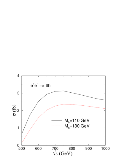
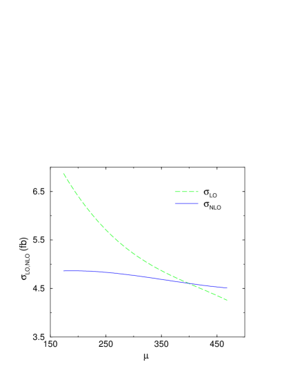
As a second example of the role of QCD in top quark physics, we consider the associated production of a tt¯𝑡¯𝑡t{\overline{t}} pair along with a Higgs boson, hh. The tt¯h𝑡¯𝑡t{\overline{t}}h Yukawa coupling is a fundamental parameter of the theory and probes the mechanism of mass generation, since in the Standard Model, gtth=Mtvsubscript𝑔𝑡𝑡subscript𝑀𝑡𝑣g_{tth}={M_{t}\over v}. The processes e+ett¯hsuperscript𝑒superscript𝑒𝑡¯𝑡e^{+}e^{-}\rightarrow t{\overline{t}}h and pp(pp¯)tt¯h𝑝𝑝𝑝¯𝑝𝑡¯𝑡pp(p{\overline{p}})\rightarrow t{\overline{t}}h provide sensitive measurements of the top quark- Higgs coupling and can be used to verify the correctness of the Standard Model and to search for new physics in the top quark and Higgs sectors. The importance of the QCD NLO corrections to tt¯h𝑡¯𝑡t{\overline{t}}h production is discussed at the end of this section.

t(p)𝑡superscript𝑝t(p^{\prime})t¯(q)¯𝑡superscript𝑞{\overline{t}}(q^{\prime})e(p)superscript𝑒𝑝e^{-}(p)e+(q)superscript𝑒𝑞e^{+}(q)γ,Z𝛾𝑍\gamma,Z
Figure 13: Lowest order Feynman diagram for e+ett¯superscript𝑒superscript𝑒𝑡¯𝑡e^{+}e^{-}\rightarrow t{\overline{t}}.

4.1 NLO QCD corrections to e+ett¯superscript𝑒superscript𝑒𝑡¯𝑡e^{+}e^{-}\rightarrow t{\overline{t}}

The Born amplitude for e+ett¯superscript𝑒superscript𝑒𝑡¯𝑡e^{+}e^{-}\rightarrow t{\overline{t}} proceeds via slimit-from𝑠s- channel γ𝛾\gamma and Z𝑍Z exchange, as shown in Fig. 13. The dominant contribution at s=500GeV𝑠500𝐺𝑒𝑉\sqrt{s}=500~{}GeV is from γ𝛾\gamma exchange and so for simplicity we will neglect the Z𝑍Z contribution here. (The complete O(αs)𝑂subscript𝛼𝑠{\it O}(\alpha_{s}) result, including the contribution from Zlimit-from𝑍Z- exchange can be found in Refs. \refcitejlz and \refciteharris.) The electron mass can also be neglected. The lowest order amplitude is:

ALO(e+ett¯)=e2QeQtsv¯(q)γμu(p)u¯(p)γμv(q)δij,subscript𝐴𝐿𝑂superscript𝑒superscript𝑒𝑡¯𝑡superscript𝑒2subscript𝑄𝑒subscript𝑄𝑡𝑠¯𝑣𝑞superscript𝛾𝜇𝑢𝑝¯𝑢superscript𝑝subscript𝛾𝜇𝑣superscript𝑞subscript𝛿𝑖𝑗{\it A}_{LO}(e^{+}e^{-}\rightarrow t{\overline{t}})={e^{2}Q_{e}Q_{t}\over s}{\overline{v}}(q)\gamma^{\mu}u(p){\overline{u}}(p^{\prime})\gamma_{\mu}v(q^{\prime})\delta_{ij}~{},

where i,j𝑖𝑗i,j are the color indices of the outgoing top quarks. It is simplest to work in the center-of-mass frame of the incoming e+esuperscript𝑒superscript𝑒e^{+}e^{-} pair, where the 4limit-from44- momenta of the particles are given by:

p𝑝\displaystyle p =\displaystyle= s2(1,0,0,1)𝑠21001\displaystyle{\sqrt{s}\over 2}(1,0,0,1)
q𝑞\displaystyle q =\displaystyle= s2(1,0,0,1)𝑠21001\displaystyle{\sqrt{s}\over 2}(1,0,0,-1)
psuperscript𝑝\displaystyle p^{\prime} =\displaystyle= s2(1,0,βsinθ,βcosθ)𝑠210𝛽𝜃𝛽𝜃\displaystyle{\sqrt{s}\over 2}(1,0,\beta\sin\theta,\beta\cos\theta)
qsuperscript𝑞\displaystyle q^{\prime} =\displaystyle= s2(1,0,βsinθ,βcosθ)𝑠210𝛽𝜃𝛽𝜃\displaystyle{\sqrt{s}\over 2}(1,0,-\beta\sin\theta,-\beta\cos\theta)

with

s𝑠\displaystyle s =\displaystyle= (p+q)2superscript𝑝𝑞2\displaystyle(p+q)^{2}
β𝛽\displaystyle\beta =\displaystyle= 14Mt2s14superscriptsubscript𝑀𝑡2𝑠\displaystyle\sqrt{1-{4M_{t}^{2}\over s}} (65)

and θ𝜃\theta is the angle of the top quark emission with respect to the electron beam direction. The threshold condition is defined by β=0𝛽0\beta=0.

It is straightforward to find the tree level amplitude-squared in n=42ϵ𝑛42italic-ϵn=4-2\epsilon dimensions, (summed over colors),

ALO2=64π2α2Qt2Nc[2(1ϵ)+β2(cos2θ1)].superscriptdelimited-∣∣subscript𝐴𝐿𝑂264superscript𝜋2superscript𝛼2superscriptsubscript𝑄𝑡2subscript𝑁𝑐delimited-[]21italic-ϵsuperscript𝛽2superscript2𝜃1\mid{\it A}_{LO}\mid^{2}=64\pi^{2}\alpha^{2}Q_{t}^{2}N_{c}\biggl{[}2(1-\epsilon)+\beta^{2}(\cos^{2}\theta-1)\biggr{]}~{}. (66)

The color factor is Nc=3subscript𝑁𝑐3N_{c}=3. The corresponding total cross section is:

σLO=12sALO2(dPS)2.subscript𝜎𝐿𝑂12𝑠superscriptdelimited-∣∣subscript𝐴𝐿𝑂2subscript𝑑𝑃𝑆2\sigma_{LO}={1\over 2s}\int\mid{\it A}_{LO}\mid^{2}(dPS)_{2}. (67)

Integrating over the two body phase space,

(dPS)2=22ϵ16π(4πs)ϵβ12ϵ1Γ(1ϵ)0πsin12ϵθdθ,subscript𝑑𝑃𝑆2superscript22italic-ϵ16𝜋superscript4𝜋𝑠italic-ϵsuperscript𝛽12italic-ϵ1Γ1italic-ϵsuperscriptsubscript0𝜋superscript12italic-ϵ𝜃𝑑𝜃(dPS)_{2}={2^{2\epsilon}\over 16\pi}\biggl{(}{4\pi\over s}\biggr{)}^{\epsilon}\beta^{1-2\epsilon}{1\over\Gamma(1-\epsilon)}\int_{0}^{\pi}\sin^{1-2\epsilon}\theta d\theta, (68)

and including a factor of 1414{1\over 4} for the average over the initial electron spins, gives a total rate,

σLO(e+ett¯)subscript𝜎𝐿𝑂superscript𝑒superscript𝑒𝑡¯𝑡\displaystyle\sigma_{LO}(e^{+}e^{-}\rightarrow t{\overline{t}}) =\displaystyle= β32πs1411dcosθALO2+O(ϵ)𝛽32𝜋𝑠14superscriptsubscript11𝑑𝜃superscriptdelimited-∣∣subscript𝐴𝐿𝑂2𝑂italic-ϵ\displaystyle{\beta\over 32\pi s}{1\over 4}\int_{-1}^{1}d\cos\theta\mid{\it A}_{LO}\mid^{2}+{\it O}(\epsilon)
=\displaystyle= 2πNcα2Qt23sβ(3β2)+O(ϵ).2𝜋subscript𝑁𝑐superscript𝛼2superscriptsubscript𝑄𝑡23𝑠𝛽3superscript𝛽2𝑂italic-ϵ\displaystyle{2\pi N_{c}\alpha^{2}Q_{t}^{2}\over 3s}\beta(3-\beta^{2})+{\it O}(\epsilon).

The O(ϵ)𝑂italic-ϵ{\it O}(\epsilon) terms which we have neglected will be important in computing the O(αs)𝑂subscript𝛼𝑠{\it O}(\alpha_{s}) QCD corrections. The cross section vanishes at threshold, β0𝛽0\beta\rightarrow 0, and decreases with increasing energy, σ1ssimilar-to𝜎1𝑠\sigma\sim{1\over s}. This has the obvious implication that the higher energy an e+esuperscript𝑒superscript𝑒e^{+}e^{-} collider, the larger the required luminosity.

4.2 O(αs)𝑂subscript𝛼𝑠{\it O}(\alpha_{s}) corrections to e+ett¯superscript𝑒superscript𝑒𝑡¯𝑡e^{+}e^{-}\rightarrow t{\overline{t}}

The O(αs)𝑂subscript𝛼𝑠{\it O}(\alpha_{s}) corrections to e+ett¯superscript𝑒superscript𝑒𝑡¯𝑡e^{+}e^{-}\rightarrow t{\overline{t}} contain both real and virtual contributions:

σNLO=σLO+σvirtual+σreal.subscript𝜎𝑁𝐿𝑂subscript𝜎𝐿𝑂subscript𝜎𝑣𝑖𝑟𝑡𝑢𝑎𝑙subscript𝜎𝑟𝑒𝑎𝑙\sigma_{NLO}=\sigma_{LO}+\sigma_{virtual}+\sigma_{real}. (69)

The one-loop virtual contribution consists of a vertex correction and a wavefunction renormalization of the top quark leg. The vertex correction is shown in Fig. 14 and can be parameterized as:

Avertex=eQev¯(q)γνu(p)1sΓν(p,q)subscript𝐴𝑣𝑒𝑟𝑡𝑒𝑥𝑒subscript𝑄𝑒¯𝑣𝑞subscript𝛾𝜈𝑢𝑝1𝑠superscriptΓ𝜈superscript𝑝superscript𝑞{\it A}_{vertex}=eQ_{e}{\overline{v}}(q)\gamma_{\nu}u(p){1\over s}\Gamma^{\nu}(p^{\prime},q^{\prime}) (70)

with,

γνsuperscript𝛾absent𝜈\gamma^{*\nu}g𝑔gt(p)𝑡superscript𝑝t(p^{\prime})t¯(q)¯𝑡superscript𝑞{\overline{t}}(q^{\prime})
Figure 14: Vertex correction to e+ett¯superscript𝑒superscript𝑒𝑡¯𝑡e^{+}e^{-}\rightarrow t{\overline{t}}. The γνsuperscript𝛾absent𝜈\gamma^{*\nu} denotes an off-shell photon which is connected to the initial e+esuperscript𝑒superscript𝑒e^{+}e^{-} state.
Γν(p,q)=(eQt)δijgs2CF[N]u¯(p)[A(p+q)ν2Mt+Bγν]v(q)subscriptΓ𝜈superscript𝑝superscript𝑞𝑒subscript𝑄𝑡subscript𝛿𝑖𝑗superscriptsubscript𝑔𝑠2subscript𝐶𝐹delimited-[]𝑁¯𝑢superscript𝑝delimited-[]𝐴subscriptsuperscript𝑝superscript𝑞𝜈2subscript𝑀𝑡𝐵subscript𝛾𝜈𝑣superscript𝑞\Gamma_{\nu}(p^{\prime},q^{\prime})=(-eQ_{t})\delta_{ij}g_{s}^{2}C_{F}[{\it N}]{\overline{u}}(p^{\prime})\biggl{[}A{(p^{\prime}+q^{\prime})_{\nu}\over 2M_{t}}+B\gamma_{\nu}\biggr{]}v(q^{\prime}) (71)

where the normalization is,

[N]116π2(4πμ2Mt2)ϵΓ(1+ϵ)delimited-[]𝑁116superscript𝜋2superscript4𝜋superscript𝜇2superscriptsubscript𝑀𝑡2italic-ϵΓ1italic-ϵ[{\it N}]\equiv{1\over 16\pi^{2}}\biggl{(}{4\pi\mu^{2}\over M_{t}^{2}}\biggr{)}^{\epsilon}\Gamma(1+\epsilon) (72)

and

CF=Nc212Nc=43.subscript𝐶𝐹superscriptsubscript𝑁𝑐212subscript𝑁𝑐43C_{F}={N_{c}^{2}-1\over 2N_{c}}={4\over 3}~{}. (73)

is the color factor for the vertex diagram. The parameter μ𝜇\mu is an arbitrary renormalization scale. Explicit calculation gives the results,[28, 30]

A𝐴\displaystyle A =\displaystyle= (β1β)Λβ𝛽1𝛽subscriptΛ𝛽\displaystyle(\beta-{1\over\beta})\Lambda_{\beta}
ΛβsubscriptΛ𝛽\displaystyle\Lambda_{\beta} \displaystyle\equiv log(1β1+β)1𝛽1𝛽\displaystyle\log\biggl{(}{1-\beta\over 1+\beta}\biggr{)}\
B𝐵\displaystyle B =\displaystyle= 1ϵ[1(1β+β)Λβ]3βΛβ+(1β+β)[12Λβ2+2Λβlog(2β1+β)\displaystyle{1\over\epsilon}\biggl{[}1-({1\over\beta}+\beta)\Lambda_{\beta}\biggr{]}-3\beta\Lambda_{\beta}+\biggl{(}{1\over\beta}+\beta\biggr{)}\biggl{[}-{1\over 2}\Lambda_{\beta}^{2}+2\Lambda_{\beta}\log\biggl{(}{2\beta\over 1+\beta}\biggr{)}
+2Li2(1β1+β)+2π23]\displaystyle+2Li_{2}({1-\beta\over 1+\beta})+{2\pi^{2}\over 3}\biggr{]}
\displaystyle\equiv Bϵϵ+Bfin.subscript𝐵italic-ϵitalic-ϵsubscript𝐵𝑓𝑖𝑛\displaystyle{B_{\epsilon}\over\epsilon}+B_{fin}~{}~{}.

The di-logarithm is defined by,

Li2(x)=01𝑑z11xz.𝐿subscript𝑖2𝑥superscriptsubscript01differential-d𝑧11𝑥𝑧Li_{2}(x)=-\int_{0}^{1}dz{1\over 1-xz}~{}. (74)

The O(αs)𝑂subscript𝛼𝑠{\it O}(\alpha_{s}) contribution to the virtual cross section is the interference of the vertex correction with the lowest order result. (The A𝐴A term of Eq. 71 does not contribute to the interference with the lowest order result when the electron mass is neglected).

σvertexsubscript𝜎𝑣𝑒𝑟𝑡𝑒𝑥\displaystyle\sigma_{vertex} =\displaystyle= 2(12s)(14)(dPS)2ALOAvertex212𝑠14subscript𝑑𝑃𝑆2subscript𝐴𝐿𝑂superscriptsubscript𝐴𝑣𝑒𝑟𝑡𝑒𝑥\displaystyle 2\biggl{(}{1\over 2s}\biggr{)}\biggl{(}{1\over 4}\biggr{)}\int(dPS)_{2}{\it A}_{LO}{\it A}_{vertex}^{*} (75)
=\displaystyle= αs2π(4πμ2Mt2)ϵCFΓ(1+ϵ)σLO[Bϵϵ+Bfin].subscript𝛼𝑠2𝜋superscript4𝜋superscript𝜇2superscriptsubscript𝑀𝑡2italic-ϵsubscript𝐶𝐹Γ1italic-ϵsubscript𝜎𝐿𝑂delimited-[]subscript𝐵italic-ϵitalic-ϵsubscript𝐵𝑓𝑖𝑛\displaystyle{\alpha_{s}\over 2\pi}\biggl{(}{4\pi\mu^{2}\over M_{t}^{2}}\biggr{)}^{\epsilon}C_{F}\Gamma(1+\epsilon)\sigma_{LO}\biggl{[}{B_{\epsilon}\over\epsilon}+B_{fin}\biggr{]}~{}~{}.

Note that the O(ϵ)𝑂italic-ϵ{\it O}(\epsilon) terms from the lowest order amplitude and from the 2-particle phase space combine with the Bϵϵsubscript𝐵italic-ϵitalic-ϵ{B_{\epsilon}\over\epsilon} term to give a finite contribution to σvertexsubscript𝜎𝑣𝑒𝑟𝑡𝑒𝑥\sigma_{vertex}.

γμsuperscript𝛾absent𝜇\gamma^{*\mu}t(p)𝑡superscript𝑝t(p^{\prime})t(q)𝑡superscript𝑞t(q^{\prime})
Figure 15: Feynman diagram for top quark wavefunction renormalization.

The wavefunction renormalization for the top quark must also be included in the virtual correction, as shown in Fig. 15. This diagram gives a multiplicative correction to the lowest order rate. Using the on-shell renormalization scheme,

σZ=2δZttσLO,subscript𝜎𝑍2𝛿subscript𝑍𝑡𝑡subscript𝜎𝐿𝑂\sigma_{Z}=2\delta Z_{tt}\sigma_{LO}, (76)

where

δZtt𝛿subscript𝑍𝑡𝑡\displaystyle\delta Z_{tt} =\displaystyle= Π(p2)p2p2=Mt2conditionalΠsuperscript𝑝2superscript𝑝2superscript𝑝2superscriptsubscript𝑀𝑡2\displaystyle{\partial\Pi(p^{2})\over\partial p^{2}}\mid p^{2}=M_{t}^{2} (77)
=\displaystyle= αs4π(4πμ2Mt2)ϵCFΓ(1+ϵ)(3ϵ+4).subscript𝛼𝑠4𝜋superscript4𝜋superscript𝜇2superscriptsubscript𝑀𝑡2italic-ϵsubscript𝐶𝐹Γ1italic-ϵ3italic-ϵ4\displaystyle-{\alpha_{s}\over 4\pi}\biggl{(}{4\pi\mu^{2}\over M_{t}^{2}}\biggr{)}^{\epsilon}C_{F}\Gamma(1+\epsilon)\biggl{(}{3\over\epsilon}+4\biggr{)}~{}.

The total virtual contribution is thus:[28, 30]

σVIRTsubscript𝜎𝑉𝐼𝑅𝑇\displaystyle\sigma_{VIRT} =\displaystyle= σvertex+σZsubscript𝜎𝑣𝑒𝑟𝑡𝑒𝑥subscript𝜎𝑍\displaystyle\sigma_{vertex}+\sigma_{Z} (78)
=\displaystyle= σLOαs2πΓ(1+ϵ)CF(4πμ2Mt2)ϵ[(3+Bϵ)1ϵ4+Bfin].subscript𝜎𝐿𝑂subscript𝛼𝑠2𝜋Γ1italic-ϵsubscript𝐶𝐹superscript4𝜋superscript𝜇2superscriptsubscript𝑀𝑡2italic-ϵdelimited-[]3subscript𝐵italic-ϵ1italic-ϵ4subscript𝐵𝑓𝑖𝑛\displaystyle\sigma_{LO}{\alpha_{s}\over 2\pi}\Gamma(1+\epsilon)C_{F}\biggl{(}{4\pi\mu^{2}\over M_{t}^{2}}\biggr{)}^{\epsilon}\biggl{[}(-3+B_{\epsilon}){1\over\epsilon}-4+B_{fin}\biggr{]}~{}.

4.3 Real contributions

The virtual singularities of Eq. 78 are cancelled by those arising from real gluon emission, e+ett¯gsuperscript𝑒superscript𝑒𝑡¯𝑡𝑔e^{+}e^{-}\rightarrow t{\overline{t}}g. A sample diagram of this type is shown in Fig. 16.

esuperscript𝑒e^{-}e+superscript𝑒e^{+}t(p)𝑡superscript𝑝t(p^{\prime})pgsubscript𝑝𝑔p_{g}t¯(q)¯𝑡superscript𝑞{\overline{t}}(q^{\prime})
Figure 16: Sample Feynman diagram for real gluon emission in the process e+ett¯gsuperscript𝑒superscript𝑒𝑡¯𝑡𝑔e^{+}e^{-}\rightarrow t{\overline{t}}g.

The real gluon emission diagram of Fig. 16 contains a fermion propagator on the outgoing top quark leg of the form:

1(p+pg)2Mt2=12ppg=12EEg(1β^cosθ^),1superscriptsuperscript𝑝subscript𝑝𝑔2superscriptsubscript𝑀𝑡212superscript𝑝subscript𝑝𝑔12superscript𝐸subscript𝐸𝑔1^𝛽^𝜃{1\over(p^{\prime}+p_{g})^{2}-M_{t}^{2}}={1\over 2p^{\prime}\cdot p_{g}}={1\over 2E^{\prime}E_{g}(1-{\hat{\beta}}\cos{\hat{\theta}})},

where Esuperscript𝐸E^{\prime} and Egsubscript𝐸𝑔E_{g} are the energies of the outgoing top quark and gluon, θ^^𝜃{\hat{\theta}} is the angle between them, and β^=1Mt2E2^𝛽1superscriptsubscript𝑀𝑡2superscript𝐸2{\hat{\beta}}=\sqrt{1-{M_{t}^{2}\over E^{\prime~{}2}}}. Because of the massive top quark, β^1^𝛽1{\hat{\beta}}\neq 1, and this diagram has no collinear singularity as θ^0^𝜃0{\hat{\theta}}\rightarrow 0. There is, however, a soft singularity as the energy of the gluon vanishes, Eg0subscript𝐸𝑔0E_{g}\rightarrow 0.

The soft singularity is regulated using a technique called phase space slicing (PSS).[30] This method divides the gluon phase space into a soft gluon plus a hard gluon region:

σrealσsoft+σhard.subscript𝜎𝑟𝑒𝑎𝑙subscript𝜎𝑠𝑜𝑓𝑡subscript𝜎𝑎𝑟𝑑\sigma_{real}\equiv\sigma_{soft}+\sigma_{hard}~{}. (79)

The soft region is defined by the energy of the emitted gluon,

Eg<δss2,subscript𝐸𝑔subscript𝛿𝑠𝑠2E_{g}<\delta_{s}{\sqrt{s}\over 2}, (80)

while the hard region is the remainder of the gluon phase space.

Eg>δss2.subscript𝐸𝑔subscript𝛿𝑠𝑠2E_{g}>\delta_{s}{\sqrt{s}\over 2}~{}. (81)

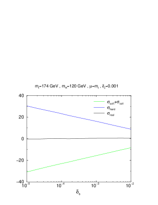
The separation into hard and soft regions depends on the arbitrary parameter δssubscript𝛿𝑠\delta_{s}. Individually, σsoftsubscript𝜎𝑠𝑜𝑓𝑡\sigma_{soft} and σhardsubscript𝜎𝑎𝑟𝑑\sigma_{hard} depend on the cutoff, δssubscript𝛿𝑠\delta_{s}, and the independence of the sum is a check on the calculation. δssubscript𝛿𝑠\delta_{s} must be small enough that terms of O(δs)𝑂subscript𝛿𝑠{\it O}(\delta_{s}) can be neglected, while large enough to prevent numerical instabilities. σhardsubscript𝜎𝑎𝑟𝑑\sigma_{hard} is finite and can be evaluated numerically using standard Monte Carlo techniques.

In the soft gluon regime, the cross section can be evaluated analytically. The three body phase space is evaluated in the soft limit in the rest frame of the incoming e+esuperscript𝑒superscript𝑒e^{+}e^{-}:

p+q=p+q+pg,𝑝𝑞superscript𝑝superscript𝑞subscript𝑝𝑔p+q=p^{\prime}+q^{\prime}+p_{g}, (82)

giving a gluon energy of

Egsubscript𝐸𝑔\displaystyle E_{g} =\displaystyle= (sspq2s)𝑠subscript𝑠superscript𝑝superscript𝑞2𝑠\displaystyle\biggl{(}{s-s_{p^{\prime}q^{\prime}}\over 2\sqrt{s}}\biggr{)}
spqsubscript𝑠superscript𝑝superscript𝑞\displaystyle s_{p^{\prime}q^{\prime}} =\displaystyle= (p+q)2.superscriptsuperscript𝑝superscript𝑞2\displaystyle(p^{\prime}+q^{\prime})^{2}~{}. (83)

The 3-body phase space in the soft limit can be separated into a 2 body phase space factor times a soft phase space factor:[31]

(dPS)3subscript𝑑𝑃𝑆3\displaystyle(dPS)_{3} =\displaystyle= dn1p2Ep(2π)n1dn1q2Eq(2π)n1(2π)nδn(p+qpqpg)superscript𝑑𝑛1superscript𝑝2subscript𝐸superscript𝑝superscript2𝜋𝑛1superscript𝑑𝑛1superscript𝑞2subscript𝐸superscript𝑞superscript2𝜋𝑛1superscript2𝜋𝑛superscript𝛿𝑛𝑝𝑞superscript𝑝superscript𝑞subscript𝑝𝑔\displaystyle\int{d^{n-1}p^{\prime}\over 2E_{p^{\prime}}(2\pi)^{n-1}}\int{d^{n-1}q^{\prime}\over 2E_{q^{\prime}}(2\pi)^{n-1}}\cdot(2\pi)^{n}\delta^{n}(p+q-p^{\prime}-q^{\prime}-p_{g}) (84)
dn1pg2Eg(2π)n1.\displaystyle~{}~{}~{}~{}\cdot\int{d^{n-1}p_{g}\over 2E_{g}(2\pi)^{n-1}}~{}~{}.

For the soft limit, we set the gluon momenta pg=0subscript𝑝𝑔0p_{g}=0 in the delta function and the phase space then factorizes:

(dPS)3(soft)=(dPS)2dn1pg2Eg(2π)n1.subscript𝑑𝑃𝑆3𝑠𝑜𝑓𝑡subscript𝑑𝑃𝑆2superscript𝑑𝑛1subscript𝑝𝑔2subscript𝐸𝑔superscript2𝜋𝑛1(dPS)_{3}(soft)=(dPS)_{2}\int{d^{n-1}p_{g}\over 2E_{g}(2\pi)^{n-1}}~{}. (85)

The phase space is most easily evaluated by choosing an explicit representation for the gluon momentum,

pg=Eg(1,,sinθ1sinθ2,sinθ1cosθ2,cosθ1).subscript𝑝𝑔subscript𝐸𝑔1subscript𝜃1subscript𝜃2subscript𝜃1subscript𝜃2subscript𝜃1p_{g}=E_{g}(1,...,\sin\theta_{1}\sin\theta_{2},\sin\theta_{1}\cos\theta_{2},\cos\theta_{1}). (86)

yielding,[32]

dn1pgsuperscript𝑑𝑛1subscript𝑝𝑔\displaystyle d^{n-1}p_{g} =\displaystyle= dpgpgn2dΩn2𝑑delimited-∣∣subscript𝑝𝑔superscriptdelimited-∣∣subscript𝑝𝑔𝑛2𝑑subscriptΩ𝑛2\displaystyle d\mid{\vec{p}_{g}}\mid\mid{\vec{p}_{g}}\mid^{n-2}d\Omega_{n-2} (87)
=\displaystyle= dEgEgn2sinn3θ1dθ1sinn4θ2dθ2dΩn4𝑑subscript𝐸𝑔superscriptsubscript𝐸𝑔𝑛2superscript𝑛3subscript𝜃1𝑑subscript𝜃1superscript𝑛4subscript𝜃2𝑑subscript𝜃2𝑑subscriptΩ𝑛4\displaystyle dE_{g}E_{g}^{n-2}\sin^{n-3}\theta_{1}d\theta_{1}\sin^{n-4}\theta_{2}d\theta_{2}d\Omega_{n-4}

where,

Ωn4=2π(n3)/2Γ(n32).subscriptΩ𝑛42superscript𝜋𝑛32Γ𝑛32\Omega_{n-4}={2\pi^{(n-3)/2}\over\Gamma({n-3\over 2})}. (88)

The integrals can be performed analytically to find the three body phase space in soft limit:[32]

(dPS)3(soft)subscript𝑑𝑃𝑆3𝑠𝑜𝑓𝑡\displaystyle(dPS)_{3}(soft) =\displaystyle= (dPS)2(4πs)ϵ(18π2)Γ(1ϵ)Γ(12ϵ)dPSsoftsubscript𝑑𝑃𝑆2superscript4𝜋𝑠italic-ϵ18superscript𝜋2Γ1italic-ϵΓ12italic-ϵ𝑑𝑃subscript𝑆𝑠𝑜𝑓𝑡\displaystyle(dPS)_{2}\biggl{(}{4\pi\over s}\biggr{)}^{\epsilon}\biggl{(}{1\over 8\pi^{2}}\biggr{)}{\Gamma(1-\epsilon)\over\Gamma(1-2\epsilon)}dPS_{soft}
dPSsoft𝑑𝑃subscript𝑆𝑠𝑜𝑓𝑡\displaystyle dPS_{soft} =\displaystyle= 1π(s4)ϵ0δss2𝑑EgEg12ϵ1𝜋superscript𝑠4italic-ϵsuperscriptsubscript0subscript𝛿𝑠𝑠2differential-dsubscript𝐸𝑔superscriptsubscript𝐸𝑔12italic-ϵ\displaystyle{1\over\pi}\biggl{(}{s\over 4}\biggr{)}^{\epsilon}\int_{0}^{\delta_{s}{\sqrt{s}\over 2}}dE_{g}E_{g}^{1-2\epsilon} (89)
sin12ϵθ1dθ1sin2ϵθ2dθ2.absentsuperscript12italic-ϵsubscript𝜃1𝑑subscript𝜃1superscript2italic-ϵsubscript𝜃2𝑑subscript𝜃2\displaystyle~{}~{}~{}~{}\cdot\sin^{1-2\epsilon}\theta_{1}d\theta_{1}\sin^{-2\epsilon}\theta_{2}d\theta_{2}~{}.

Note that the soft phase space depends explicitely on the cut-off δssubscript𝛿𝑠\delta_{s} through the limit on the Egsubscript𝐸𝑔E_{g} integral.

The soft phase space must be combined with the amplitude for e+ett¯gsuperscript𝑒superscript𝑒𝑡¯𝑡𝑔e^{+}e^{-}\rightarrow t{\overline{t}}g in pg0subscript𝑝𝑔0p_{g}\rightarrow 0 limit:

Asoftsubscript𝐴𝑠𝑜𝑓𝑡\displaystyle{\it A}_{soft} =\displaystyle= e2QeQtsgsTAv¯(q)γμu(p)superscript𝑒2subscript𝑄𝑒subscript𝑄𝑡𝑠subscript𝑔𝑠superscript𝑇𝐴¯𝑣𝑞subscript𝛾𝜇𝑢𝑝\displaystyle{e^{2}Q_{e}Q_{t}\over s}g_{s}T^{A}{\overline{v}}(q)\gamma_{\mu}u(p) (90)
u¯(p){γσ(p+pg+Mt)(p+pg)2Mt2γμ+γμ(qpg+Mt)(q+pg)2Mt2γσ}v(q)absent¯𝑢superscript𝑝superscript𝛾𝜎superscript𝑝subscript𝑝𝑔subscript𝑀𝑡superscriptsuperscript𝑝subscript𝑝𝑔2superscriptsubscript𝑀𝑡2superscript𝛾𝜇superscript𝛾𝜇superscript𝑞subscript𝑝𝑔subscript𝑀𝑡superscriptsuperscript𝑞subscript𝑝𝑔2superscriptsubscript𝑀𝑡2superscript𝛾𝜎𝑣superscript𝑞\displaystyle~{}~{}~{}~{}\cdot{\overline{u}}(p^{\prime})\biggl{\{}\gamma^{\sigma}{(p^{\prime}+p_{g}+M_{t})\over(p^{\prime}+p_{g})^{2}-M_{t}^{2}}\gamma^{\mu}+\gamma^{\mu}{(-q^{\prime}-p_{g}+M_{t})\over(q^{\prime}+p_{g})^{2}-M_{t}^{2}}\gamma^{\sigma}\biggr{\}}v(q^{\prime})
\displaystyle\rightarrow gsTA[pσppgqσqpg]ALOsubscript𝑔𝑠superscript𝑇𝐴delimited-[]superscript𝑝𝜎superscript𝑝subscript𝑝𝑔superscript𝑞𝜎superscript𝑞subscript𝑝𝑔subscript𝐴𝐿𝑂\displaystyle g_{s}T^{A}\biggl{[}{p^{\prime\sigma}\over p^{\prime}\cdot p_{g}}-{q^{\prime\sigma}\over q^{\prime}\cdot p_{g}}\biggr{]}{\it A}_{LO}

where we have set pg=0subscript𝑝𝑔0p_{g}=0 in the numerator. The approximation of retaining only the most singular contributions is known as the eikonal ( or double pole) approximation.[33] The soft limit of the amplitude always factorizes in this manner into a factor multiplying the lowest order amplitude.

The soft amplitude-squared is

Asoft2superscriptdelimited-∣∣subscript𝐴𝑠𝑜𝑓𝑡2\displaystyle\mid{\it A}_{soft}\mid^{2} =\displaystyle= gs2Tr(TATA)ALO2superscriptsubscript𝑔𝑠2𝑇𝑟superscript𝑇𝐴superscript𝑇𝐴superscriptdelimited-∣∣subscript𝐴𝐿𝑂2\displaystyle g_{s}^{2}Tr(T^{A}T^{A})\mid{\it A}_{LO}\mid^{2} (91)
[Mt2(ppg)2Mt2(qpg)2+s2Mt2ppgqpg]absentdelimited-[]superscriptsubscript𝑀𝑡2superscriptsuperscript𝑝subscript𝑝𝑔2superscriptsubscript𝑀𝑡2superscriptsuperscript𝑞subscript𝑝𝑔2𝑠2superscriptsubscript𝑀𝑡2superscript𝑝subscript𝑝𝑔superscript𝑞subscript𝑝𝑔\displaystyle~{}~{}~{}~{}~{}\cdot\biggl{[}-{M_{t}^{2}\over(p^{\prime}\cdot p_{g})^{2}}-{M_{t}^{2}\over(q^{\prime}\cdot p_{g})^{2}}+{s-2M_{t}^{2}\over p^{\prime}\cdot p_{g}q^{\prime}\cdot p_{g}}\biggr{]}

giving the cross section in the soft limit,333As always, the factor of 1/4141/4 is the spin average.

σsoft=12s(14)Asoft2(dPS)3(soft).subscript𝜎𝑠𝑜𝑓𝑡12𝑠14superscriptdelimited-∣∣subscript𝐴𝑠𝑜𝑓𝑡2subscript𝑑𝑃𝑆3𝑠𝑜𝑓𝑡\sigma_{soft}={1\over 2s}\biggl{(}{1\over 4}\biggr{)}\int\mid{\it A}_{soft}\mid^{2}(dPS)_{3}(soft)~{}. (92)

The problem reduces to evaluating the soft integrals. A typical integral is

Isoft1(ppg)2𝑑PS3(soft).superscript𝐼𝑠𝑜𝑓𝑡1superscriptsuperscript𝑝subscript𝑝𝑔2differential-d𝑃subscript𝑆3𝑠𝑜𝑓𝑡I^{soft}\equiv\int{1\over(p^{\prime}\cdot p_{g})^{2}}dPS_{3}(soft)~{}. (93)

Since the phase space and the amplitude squared are Lorentz invariant, we are free to chose any convenient frame. We use

pgsubscript𝑝𝑔\displaystyle p_{g} =\displaystyle= Eg(1,sinθ1sinθ2,sinθ1cosθ2,cosθ1)subscript𝐸𝑔1subscript𝜃1subscript𝜃2subscript𝜃1subscript𝜃2subscript𝜃1\displaystyle E_{g}(1,...\sin\theta_{1}\sin\theta_{2},\sin\theta_{1}\cos\theta_{2},\cos\theta_{1})
psuperscript𝑝\displaystyle p^{\prime} =\displaystyle= s2(1,0,0,β)𝑠2100𝛽\displaystyle{\sqrt{s}\over 2}(1,0,0,\beta) (94)

and the soft integral is,

Isoftsuperscript𝐼𝑠𝑜𝑓𝑡\displaystyle I^{soft} =\displaystyle= 1(ppg)2𝑑PS3(soft)1superscriptsuperscript𝑝subscript𝑝𝑔2differential-d𝑃subscript𝑆3𝑠𝑜𝑓𝑡\displaystyle\int{1\over(p^{\prime}\cdot p_{g})^{2}}dPS_{3}(soft) (95)
=\displaystyle= 1π(s4)ϵ0δss2𝑑EgEg12ϵsin12ϵθ1dθ1sin2ϵdθ21𝜋superscript𝑠4italic-ϵsuperscriptsubscript0subscript𝛿𝑠𝑠2differential-dsubscript𝐸𝑔superscriptsubscript𝐸𝑔12italic-ϵsuperscript12italic-ϵsubscript𝜃1𝑑subscript𝜃1superscript2italic-ϵ𝑑subscript𝜃2\displaystyle{1\over\pi}\biggl{(}{s\over 4}\biggr{)}^{\epsilon}\int_{0}^{\delta_{s}{\sqrt{s}\over 2}}dE_{g}E_{g}^{1-2\epsilon}\sin^{1-2\epsilon}\theta_{1}d\theta_{1}\sin^{-2\epsilon}d\theta_{2}
(4sEg2)1(1βcosθ1)2absent4𝑠superscriptsubscript𝐸𝑔21superscript1𝛽subscript𝜃12\displaystyle\cdot\biggl{(}{4\over sE_{g}^{2}}\biggr{)}{1\over(1-\beta\cos\theta_{1})^{2}}
=\displaystyle= 2Mt2(12ϵ+log(δs)+12βΛβ)+O(δs,ϵ).2superscriptsubscript𝑀𝑡212italic-ϵsubscript𝛿𝑠12𝛽subscriptΛ𝛽𝑂subscript𝛿𝑠italic-ϵ\displaystyle{2\over M_{t}^{2}}\biggl{(}-{1\over 2\epsilon}+\log(\delta_{s})+{1\over 2\beta}\Lambda_{\beta}\biggr{)}+{\it O}(\delta_{s},\epsilon)~{}.

The complete set of soft integrals relevant for this process is given in the appendix of Ref. \refciterdw.

The soft cross section is

σsoftsubscript𝜎𝑠𝑜𝑓𝑡\displaystyle\sigma_{soft} =\displaystyle= σLOαs2πCF(4πμ2s)ϵΓ(1ϵ)Γ(12ϵ)[Cϵϵ+Cfin],subscript𝜎𝐿𝑂subscript𝛼𝑠2𝜋subscript𝐶𝐹superscript4𝜋superscript𝜇2𝑠italic-ϵΓ1italic-ϵΓ12italic-ϵdelimited-[]subscript𝐶italic-ϵitalic-ϵsubscript𝐶𝑓𝑖𝑛\displaystyle\sigma_{LO}{\alpha_{s}\over 2\pi}C_{F}\biggl{(}{4\pi\mu^{2}\over s}\biggr{)}^{\epsilon}{\Gamma(1-\epsilon)\over\Gamma(1-2\epsilon)}\biggl{[}{C_{\epsilon}\over\epsilon}+C_{fin}\biggr{]}, (96)

where Bϵ=Cϵsubscript𝐵italic-ϵsubscript𝐶italic-ϵB_{\epsilon}=-C_{\epsilon} so the sum of virtual plus soft contributions is finite. The finite contribution, Cfinsubscript𝐶𝑓𝑖𝑛C_{fin}, depends on δssubscript𝛿𝑠\delta_{s} and is given by[30]

Cfinsubscript𝐶𝑓𝑖𝑛\displaystyle C_{fin} =\displaystyle= 4log(δs)2βΛβ2(1β+β)4subscript𝛿𝑠2𝛽subscriptΛ𝛽21𝛽𝛽\displaystyle-4\log(\delta_{s})-{2\over\beta}\Lambda_{\beta}-2\biggl{(}{1\over\beta}+\beta\biggr{)} (97)
[Li2(2β1+β)+Λβ24+log(δs)Λβ]+O(δs).absentdelimited-[]𝐿subscript𝑖22𝛽1𝛽superscriptsubscriptΛ𝛽24subscript𝛿𝑠subscriptΛ𝛽𝑂subscript𝛿𝑠\displaystyle\cdot\biggl{[}Li_{2}\biggl{(}{2\beta\over 1+\beta}\biggr{)}+{\Lambda_{\beta}^{2}\over 4}+\log(\delta_{s})\Lambda_{\beta}\biggr{]}+{\it O}(\delta_{s})~{}.

The complete O(αs)𝑂subscript𝛼𝑠{\it O}(\alpha_{s}) result for e+ett¯superscript𝑒superscript𝑒𝑡¯𝑡e^{+}e^{-}\rightarrow t{\overline{t}} is then,

σNLO=σLO+σvirtual+σsoft+σhard.subscript𝜎𝑁𝐿𝑂subscript𝜎𝐿𝑂subscript𝜎𝑣𝑖𝑟𝑡𝑢𝑎𝑙subscript𝜎𝑠𝑜𝑓𝑡subscript𝜎𝑎𝑟𝑑\sigma_{NLO}=\sigma_{LO}+\sigma_{virtual}+\sigma_{soft}+\sigma_{hard}~{}. (98)

The combination σsoft+σhardsubscript𝜎𝑠𝑜𝑓𝑡subscript𝜎𝑎𝑟𝑑\sigma_{soft}+\sigma_{hard} is independent of δssubscript𝛿𝑠\delta_{s}, while the 1ϵ1italic-ϵ{1\over\epsilon} poles cancel between σsoft+σvirtualsubscript𝜎𝑠𝑜𝑓𝑡subscript𝜎𝑣𝑖𝑟𝑡𝑢𝑎𝑙\sigma_{soft}+\sigma_{virtual}.

This example, e+ett¯superscript𝑒superscript𝑒𝑡¯𝑡e^{+}e^{-}\rightarrow t{\overline{t}}, is simple enough that it could have been done analytically without the approximation of phase space slicing[28]. Phase space slicing, however, is useful for more complicated examples and also to construct Monte Carlo distributions beyond the leading order.

4.4 Threshold Scan in e+ett¯superscript𝑒superscript𝑒𝑡¯𝑡e^{+}e^{-}\rightarrow t{\overline{t}}

The energy dependence of the cross section for e+ett¯superscript𝑒superscript𝑒𝑡¯𝑡e^{+}e^{-}\rightarrow t{\overline{t}} at threshold depends sensitively on the parameters of the top sector. The location of the peak depends on Mtsubscript𝑀𝑡M_{t}, while the height of the peak depends on ΓtsubscriptΓ𝑡\Gamma_{t}. The problem is that the location of the peak as a function of center-of-mass energy shifts at higher orders and there is a large renormalization scale dependence to the prediction as seen in Fig. 17.[35]

At threshold, β0𝛽0\beta\rightarrow 0, the theory possesses two small parameters: αssubscript𝛼𝑠\alpha_{s} and β𝛽\beta and the cross section diverges at O(αs)𝑂subscript𝛼𝑠{\it O}(\alpha_{s}),[9]

σ(e+ett¯)β0=σLO(1+2παs3β).evaluated-at𝜎superscript𝑒superscript𝑒𝑡¯𝑡𝛽0subscript𝜎𝐿𝑂12𝜋subscript𝛼𝑠3𝛽\sigma(e^{+}e^{-}\rightarrow t{\overline{t}})\mid_{\beta\rightarrow 0}=\sigma_{LO}\biggl{(}1+{2\pi\alpha_{s}\over 3\beta}\biggr{)}. (99)

This divergence as β0𝛽0\beta\rightarrow 0 is known as a Coulomb singularity and non-relativistic quantum mechanics can be used to sum the leading contributions in powers of 1β1𝛽{1\over\beta}.[36]

Beyond lowest order in αssubscript𝛼𝑠\alpha_{s}, the predictions are quite sensitive to the precise definition of the top quark mass. The most straightforward definition is the pole mass appearing in the top quark propagator,
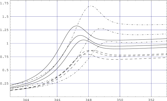
Refer to caption
Figure 17: Cross section for e+ett¯superscript𝑒superscript𝑒𝑡¯𝑡e^{+}e^{-}\rightarrow t{\overline{t}} as a function of the center-of-mass energy in GeV using the pole mass definition for the top quark mass at lowest order ( dot-dashed), NLO (dashed), and NNLO (solid). The vertical axis shows σ(e+ett¯)/σpt𝜎superscript𝑒superscript𝑒𝑡¯𝑡subscript𝜎𝑝𝑡\sigma(e^{+}e^{-}\rightarrow t{\overline{t}})/\sigma_{pt}, where σpt=4πα2/3ssubscript𝜎𝑝𝑡4𝜋superscript𝛼23𝑠\sigma_{pt}=4\pi\alpha^{2}/3s. The three sets of curves at each order represent the variation with the renormalization scale μ𝜇\mu, (μ=15,30,𝜇1530\mu=15,~{}30, and 60GeV60𝐺𝑒𝑉60~{}GeV).[37]
D(p)=ipMtpoleΣ(p).𝐷𝑝𝑖𝑝evaluated-atsubscript𝑀𝑡𝑝𝑜𝑙𝑒Σ𝑝D(p)={i\over p-M_{t}\mid_{pole}-\Sigma(p)}~{}. (100)

The pole mass, Mtpoleevaluated-atsubscript𝑀𝑡𝑝𝑜𝑙𝑒M_{t}\mid_{pole}, is measured by reconstructing the four-momenta of top quark decay products. This definition of the top quark mass is, however, uncertain by QCD hadronization effects, O(ΛQCD)𝑂subscriptΛ𝑄𝐶𝐷{\it O}(\Lambda_{QCD}). These effects connect the top quark with its decay products. Even more disturbing is the fact that the location and height of the peak in the e+ett¯superscript𝑒superscript𝑒𝑡¯𝑡e^{+}e^{-}\rightarrow t{\overline{t}} cross section change significantly between lowest order, NLO, and NNLO as seen in Fig. 17. A better definition of the top quark mass is the short distance 1S1𝑆1S mass:[37, 38]

m1S=Mtpole(12αs29.).m_{1S}=M_{t}\mid_{pole}(1-{2\alpha_{s}^{2}\over 9}....)~{}. (101)

Using this mass definition, the cross section for e+ett¯superscript𝑒superscript𝑒𝑡¯𝑡e^{+}e^{-}\rightarrow t{\overline{t}} peaks at 2m1S2subscript𝑚1𝑆2m_{1S} and the location of the peak does not shift at NLO or NNLO, as seen in Fig. 18.
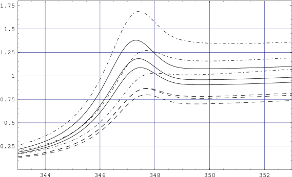
Refer to caption
Figure 18: Cross section for e+ett¯superscript𝑒superscript𝑒𝑡¯𝑡e^{+}e^{-}\rightarrow t{\overline{t}} as a function of the center-of-mass energy in GeV using the 1S mass definition for the top quark mass at lowest order ( dot-dashed), NLO (dashed), and NNLO (solid). The vertical axis shows σ(e+ett¯)/σpt𝜎superscript𝑒superscript𝑒𝑡¯𝑡subscript𝜎𝑝𝑡\sigma(e^{+}e^{-}\rightarrow t{\overline{t}})/\sigma_{pt}, where σpt=4πα2/3ssubscript𝜎𝑝𝑡4𝜋superscript𝛼23𝑠\sigma_{pt}=4\pi\alpha^{2}/3s. The three sets of curves at each order represent the variation with the renormalization scale μ𝜇\mu, (μ=15,30,𝜇1530\mu=15,~{}30, and 60GeV60𝐺𝑒𝑉60~{}GeV). [37]

The NNLO result still has roughly a 20%percent2020\% scale uncertainty. It is estimated that by scanning the threshold dependence of the cross section for e+ett¯superscript𝑒superscript𝑒𝑡¯𝑡e^{+}e^{-}\rightarrow t{\overline{t}} a measurement with the accuracy δMt200MeVsimilar-to𝛿subscript𝑀𝑡200𝑀𝑒𝑉\delta M_{t}\sim 200~{}MeV can be made with an integrated luminosity of L=50fb1𝐿50𝑓superscript𝑏1{\it L}=50~{}fb^{-1}. This is to be compared with the expected accuracy of the LHC measurement, δMt12GeVsimilar-to𝛿subscript𝑀𝑡12𝐺𝑒𝑉\delta M_{t}\sim 1-2~{}GeV.[26] A precise measurement of the top quark mass is of interest primarily because of its implications for electroweak precision measurements.[25]

4.5 tth𝑡𝑡tth production in e+esuperscript𝑒superscript𝑒e^{+}e^{-} and pp𝑝𝑝pp collisions

In many models with physics beyond the Standard Model, the Higgs coupling to the top quark is significantly different from that in the Standard Model. In the Standard Model, the fermion-Higgs Yukawa couplings are,

L=gffhψ¯ψh𝐿subscript𝑔𝑓𝑓¯𝜓𝜓{\it L}=-g_{ffh}{\overline{\psi}}\psi h (102)

where

gffh=Mfv.subscript𝑔𝑓𝑓subscript𝑀𝑓𝑣g_{ffh}={M_{f}\over v}~{}. (103)

Since the top quark is the heaviest quark, it has the largest Yukawa coupling to the Higgs boson. It is important to measure this coupling accurately in order to verify that the Higgs mechanism is the source of fermion masses.

The Higgs boson couplings to the lighter quarks can be tested by measuring the Higgs decays to fermion pairs. This is not possible, however, for the top-fermion coupling. Only for very heavy Higgs bosons (Mh>2Mtsubscript𝑀2subscript𝑀𝑡M_{h}>2M_{t}) is the decay htt¯𝑡¯𝑡h\rightarrow t{\overline{t}} kinematically accessible, and the branching ratio of the Higgs into tt¯𝑡¯𝑡t{\overline{t}} pairs is significantly smaller than that into gauge boson pairs. It does not appear feasible to measure gtthsubscript𝑔𝑡𝑡g_{tth} through this channel. The most promising prospect for measuring the top quark Yukawa coupling is tt¯h𝑡¯𝑡t{\overline{t}}h production in e+esuperscript𝑒superscript𝑒e^{+}e^{-} and pp𝑝𝑝pp (or pp¯𝑝¯𝑝p{\overline{p}}) collisions.

4.6 tt¯h𝑡¯𝑡t{\overline{t}}h at an e+esuperscript𝑒superscript𝑒e^{+}e^{-} collider

At an e+esuperscript𝑒superscript𝑒e^{+}e^{-} collider, tt¯h𝑡¯𝑡t{\overline{t}}h associated production occurs through s𝑠s-channel γ𝛾\gamma and Z𝑍Z exchange, as shown in Fig. 19.

γ,Z𝛾𝑍\gamma,Zesuperscript𝑒e^{-}e+superscript𝑒e^{+}hht𝑡tt¯¯𝑡{\overline{t}}
Z𝑍Zesuperscript𝑒e^{-}e+superscript𝑒e^{+}hht𝑡tt¯¯𝑡{\overline{t}}
Figure 19: Contributions to e+ett¯hsuperscript𝑒superscript𝑒𝑡¯𝑡e^{+}e^{-}\rightarrow t{\overline{t}}h at lowest order.

The contribution from Z𝑍Z exchange is a few percent of the total rate and will be neglected here. With this assumption, the rate is directly proportional to gtth2superscriptsubscript𝑔𝑡𝑡2g_{tth}^{2}. In order to interpret the cross section as a measurement of gtthsubscript𝑔𝑡𝑡g_{tth}, however, it is necessary to include the QCD corrections which are potentially of the same order of magnitude as new physics effects which may change gtthsubscript𝑔𝑡𝑡g_{tth} from the SM prediction. The NLO QCD result includes virtual and real gluon corrections on the outgoing t,t¯𝑡¯𝑡t,{\overline{t}} legs. The calculation follows that of the previous section for e+ett¯superscript𝑒superscript𝑒𝑡¯𝑡e^{+}e^{-}\rightarrow t{\overline{t}}, although in this case the virtual calculation also includes box diagrams. These corrections have been found in Refs. \refciteeetth_QCD1 and \refciteeetth_QCD2 and can be parameterized as

KσNLOσLO=1+αs(μ)F(s,Mt2,Mh2).𝐾subscript𝜎𝑁𝐿𝑂subscript𝜎𝐿𝑂1subscript𝛼𝑠𝜇𝐹𝑠superscriptsubscript𝑀𝑡2superscriptsubscript𝑀2K\equiv{\sigma_{NLO}\over\sigma_{LO}}=1+\alpha_{s}(\mu)F(s,M_{t}^{2},M_{h}^{2})~{}~{}. (104)

The parameter μ𝜇\mu is an unphysical renormalization scale and, at this order, the only dependence on μ𝜇\mu is in the running of αs(μ)subscript𝛼𝑠𝜇\alpha_{s}(\mu). For Mh=120GeVsubscript𝑀120𝐺𝑒𝑉M_{h}=120~{}GeV, and μ𝜇\mu ranging from Mtsubscript𝑀𝑡M_{t} to s𝑠\sqrt{s},

K(s=500GeV)𝐾𝑠500𝐺𝑒𝑉\displaystyle K(\sqrt{s}=500~{}GeV) similar-to\displaystyle\sim 1.41.51.41.5\displaystyle 1.4-1.5
K(s=1TeV)𝐾𝑠1𝑇𝑒𝑉\displaystyle K(\sqrt{s}=1~{}TeV) similar-to\displaystyle\sim .8.9..8.9\displaystyle.8-.9~{}. (105)

The NLO results for tt¯h𝑡¯𝑡t{\overline{t}}h production in e+esuperscript𝑒superscript𝑒e^{+}e^{-} collisions are shown in Fig. 20. The rate is quite small and has a maximum value for s700800GeVsimilar-to𝑠700800𝐺𝑒𝑉\sqrt{s}\sim 700-800~{}GeV for Mhsubscript𝑀M_{h} in the 120GeV120𝐺𝑒𝑉120~{}GeV region.

.

Refer to caption
Figure 20: NLO rate for e+ett¯hsuperscript𝑒superscript𝑒𝑡¯𝑡e^{+}e^{-}\rightarrow t{\overline{t}}h as a function of center of mass energy.[39]

In order to measure the top quark Yukawa coupling in e+esuperscript𝑒superscript𝑒e^{+}e^{-} collisions, we consider the final state

e+ett¯hW+Wbb¯bb¯.superscript𝑒superscript𝑒𝑡¯𝑡superscript𝑊superscript𝑊𝑏¯𝑏𝑏¯𝑏e^{+}e^{-}\rightarrow t{\overline{t}}h\rightarrow W^{+}W^{-}b{\overline{b}}b{\overline{b}}~{}. (106)

The events are then classified according to the W𝑊W decays, in an analogous manner to that discussed in Section 3.5 for top quark decays. Since the event rate is quite small, it is advantageous to combine hadronic and semi-leptonic W𝑊W decay channels.[41, 42] At s=800GeV𝑠800𝐺𝑒𝑉\sqrt{s}=800~{}GeV , an integrated luminosity of L=1000fb1𝐿1000𝑓superscript𝑏1{\it L}=1000~{}fb^{-1}, can measure the coupling to an accuracy of[41]

δgtthgtth5.5%.similar-to𝛿subscript𝑔𝑡𝑡subscript𝑔𝑡𝑡percent5.5{\delta g_{tth}\over g_{tth}}\sim 5.5\%~{}. (107)

At a lower energy, s=500GeV𝑠500𝐺𝑒𝑉\sqrt{s}=500~{}GeV, the rate is considerably smaller and even with an integrated luminosity of L=1000fb1𝐿1000𝑓superscript𝑏1{\it L}=1000~{}fb^{-1}, the precision is quite poor,[42]

δgtthgtth20%,similar-to𝛿subscript𝑔𝑡𝑡subscript𝑔𝑡𝑡percent20{\delta g_{tth}\over g_{tth}}\sim 20\%~{}, (108)

for Mh=120GeVsubscript𝑀120𝐺𝑒𝑉M_{h}=120~{}GeV.

4.7 pptt¯h𝑝𝑝𝑡¯𝑡pp\rightarrow t{\overline{t}}h at NLO

The QCD corrections to pptt¯h𝑝𝑝𝑡¯𝑡p{p}\rightarrow t{\overline{t}}h (or pp¯tt¯h𝑝¯𝑝𝑡¯𝑡p{\overline{p}}\rightarrow t{\overline{t}}h) can be calculated in a similar fashion to those for e+ett¯hsuperscript𝑒superscript𝑒𝑡¯𝑡e^{+}e^{-}\rightarrow t{\overline{t}}h. In the hadronic case, however, the calculation is complicated by the existence of strong interactions in the initial state. In this section, we discuss the treatment of initial state singularities in hadron collisions. The ingredients of an NLO calculation for pp𝑝𝑝pp or pp¯tt¯h𝑝¯𝑝𝑡¯𝑡p{\overline{p}}\rightarrow t{\overline{t}}h are:[34, 43]

  • σvirtual::subscript𝜎𝑣𝑖𝑟𝑡𝑢𝑎𝑙absent\sigma_{virtual}: This contains all of the one-loop diagrams contributing to the process. Finite diagrams, or diagrams which contain only ultraviolet singularities, can be evaluated numerically.[44] Diagrams which contain infrared singularities must be evaluated analytically.

  • σsoftsubscript𝜎𝑠𝑜𝑓𝑡\sigma_{soft}: This contains the soft singularities arising from both the initial and final state soft gluon radiation in the limit pg0subscript𝑝𝑔0p_{g}\rightarrow 0. The calculation is analogous to the discussion of Section 4.3.

  • σhard::subscript𝜎𝑎𝑟𝑑absent\sigma_{hard}: This is the contribution from real gluon radiation when the gluon has an energy above the soft cut-off. In contrast to the e+esuperscript𝑒superscript𝑒e^{+}e^{-} example of Section 4.3, this contribution has a singularity when the initial state quark or gluon is parallel to the radiated final state gluon. The initial state collinear singularities are absorbed into the parton distribution functions (PDFs).

The combination σsoft+σhard+σvirtualsubscript𝜎𝑠𝑜𝑓𝑡subscript𝜎𝑎𝑟𝑑subscript𝜎𝑣𝑖𝑟𝑡𝑢𝑎𝑙\sigma_{soft}+\sigma_{hard}+\sigma_{virtual} is finite.

Refer to caption
Figure 21: NLO QCD corrections to pp¯tt¯h𝑝¯𝑝𝑡¯𝑡p{\overline{p}}\rightarrow t{\overline{t}}h at S=2TeV𝑆2𝑇𝑒𝑉\sqrt{S}=2~{}TeV. This figure shows the independence of the total cross section on the soft cutoff, δssubscript𝛿𝑠\delta_{s}.[34]

4.8 Collinear Singularities and Phase Space Slicing

To illustrate the effects of collinear singularities, we consider the parton level subprocess,

q(p)+q¯(q)t(pt)+t¯(pt)+h(ph)+g(pg).𝑞𝑝¯𝑞𝑞𝑡subscript𝑝𝑡¯𝑡subscript𝑝superscript𝑡subscript𝑝𝑔subscript𝑝𝑔q(p)+{\overline{q}}(q)\rightarrow t(p_{t})+{\overline{t}}(p_{t^{\prime}})+h(p_{h})+g(p_{g})~{}. (109)

As in the e+esuperscript𝑒superscript𝑒e^{+}e^{-} example, we divide the gluon phase space into a soft and a hard region. We then further divide σhardsubscript𝜎𝑎𝑟𝑑\sigma_{hard} into a region with collinear divergences and a finite region,

σhardσhardcoll+σhardnotcollsubscript𝜎𝑎𝑟𝑑evaluated-atsubscript𝜎𝑎𝑟𝑑𝑐𝑜𝑙𝑙evaluated-atsubscript𝜎𝑎𝑟𝑑𝑛𝑜𝑡𝑐𝑜𝑙𝑙\sigma_{hard}\equiv\sigma_{hard}\mid_{coll}+\sigma_{hard}\mid_{not-coll} (110)

The separation depends on a new cut-off, δcsubscript𝛿𝑐\delta_{c}, although σhardsubscript𝜎𝑎𝑟𝑑\sigma_{hard} must be independent of δcsubscript𝛿𝑐\delta_{c}. If the emitted gluon is from the initial state quark line, then there is a quark propagator,

1(ppg)2=12ppg=1sEg(1cosθ)1superscript𝑝subscript𝑝𝑔212𝑝subscript𝑝𝑔1𝑠subscript𝐸𝑔1𝜃{1\over(p-p_{g})^{2}}=-{1\over 2p\cdot p_{g}}=-{1\over\sqrt{s}E_{g}(1-\cos\theta)} (111)

which becomes singular when p𝑝p and pgsubscript𝑝𝑔p_{g} are parallel (cosθ1𝜃1\cos\theta\rightarrow 1). The hard/not-collinear region is defined by,

2ppgEgs>δc2qpgEgs>δc.formulae-sequence2𝑝subscript𝑝𝑔subscript𝐸𝑔𝑠subscript𝛿𝑐2𝑞subscript𝑝𝑔subscript𝐸𝑔𝑠subscript𝛿𝑐{2p\cdot p_{g}\over E_{g}\sqrt{s}}>\delta_{c}\qquad\qquad{2q\cdot p_{g}\over E_{g}\sqrt{s}}>\delta_{c}~{}. (112)

In this region the quark propagator of Eq. 111 is finite and the cross section can be computed numerically.

In the collinear region,

2ppgEgs<δc2qpgEgs<δc,formulae-sequence2𝑝subscript𝑝𝑔subscript𝐸𝑔𝑠subscript𝛿𝑐2𝑞subscript𝑝𝑔subscript𝐸𝑔𝑠subscript𝛿𝑐{2p\cdot p_{g}\over E_{g}\sqrt{s}}<\delta_{c}\qquad\qquad{2q\cdot p_{g}\over E_{g}\sqrt{s}}<\delta_{c}, (113)

and the matrix element factorizes into a parton i𝑖i splitting into a hard parton isuperscript𝑖i^{\prime} plus a collinear gluon with kinematics

p𝑝pzp𝑧𝑝zp(1z)p1𝑧𝑝(1-z)pq𝑞q
Figure 22: Diagram contributing to collinear singularity for the process qq¯tt¯hg𝑞¯𝑞𝑡¯𝑡𝑔q{\overline{q}}\rightarrow t{\overline{t}}hg.
pisubscript𝑝superscript𝑖\displaystyle p_{i^{\prime}} =\displaystyle= zpi𝑧subscript𝑝𝑖\displaystyle zp_{i}
pgsubscript𝑝𝑔\displaystyle p_{g} =\displaystyle= (1z)pi1𝑧subscript𝑝𝑖\displaystyle(1-z)p_{i}
sigsubscript𝑠𝑖𝑔\displaystyle s_{ig} \displaystyle\equiv 2pipg2subscript𝑝𝑖subscript𝑝𝑔\displaystyle 2p_{i}\cdot p_{g}

These kinematics are illustrated in Fig. 22. In the current example, qqg𝑞𝑞𝑔q\rightarrow qg and the matrix element factorizes,[34]

A(ijtt¯h+g)2collinearΣigs2ALO(ijtt¯h)22Pii(z)zsigsubscript𝑐𝑜𝑙𝑙𝑖𝑛𝑒𝑎𝑟superscriptdelimited-∣∣𝐴𝑖𝑗𝑡¯𝑡𝑔2subscriptΣsuperscript𝑖superscriptsubscript𝑔𝑠2superscriptdelimited-∣∣subscript𝐴𝐿𝑂superscript𝑖𝑗𝑡¯𝑡22subscript𝑃𝑖superscript𝑖𝑧𝑧subscript𝑠𝑖𝑔\mid{\it A}(ij\rightarrow t{\overline{t}}h+g)\mid^{2}\rightarrow_{collinear}\Sigma_{i^{\prime}}g_{s}^{2}\mid{\it A}_{LO}(i^{\prime}j\rightarrow t{\overline{t}}h)\mid^{2}{2P_{ii^{\prime}}(z)\over zs_{ig}} (114)

where Piisubscript𝑃𝑖superscript𝑖P_{ii^{\prime}} is the probability that parton i𝑖i splits into parton isuperscript𝑖i^{\prime}, with fraction z𝑧z of the initial momentum. In this example,

Pii(z)=Pqq(z)=CF[1+z21zϵ(1z)].subscript𝑃𝑖superscript𝑖𝑧subscript𝑃𝑞𝑞𝑧subscript𝐶𝐹delimited-[]1superscript𝑧21𝑧italic-ϵ1𝑧P_{ii^{\prime}}(z)=P_{qq}(z)=C_{F}\biggl{[}{1+z^{2}\over 1-z}-\epsilon(1-z)\biggr{]}~{}. (115)

The phase space also factorizes in the collinear limit:[31]

(PS)4(ijtt¯h+g)collinear(PS)3(ijtt¯h)Γ(1ϵ)Γ(12ϵ)(4π)ϵ16π2subscript𝑃𝑆4subscript𝑖𝑗𝑡¯𝑡𝑔𝑐𝑜𝑙𝑙𝑖𝑛𝑒𝑎𝑟subscript𝑃𝑆3superscript𝑖𝑗𝑡¯𝑡Γ1italic-ϵΓ12italic-ϵsuperscript4𝜋italic-ϵ16superscript𝜋2\displaystyle(PS)_{4}(ij\rightarrow t{\overline{t}}h+g)_{collinear}\rightarrow(PS)_{3}(i^{\prime}j\rightarrow t{\overline{t}}h){\Gamma(1-\epsilon)\over\Gamma(1-2\epsilon)}{(4\pi)^{\epsilon}\over 16\pi^{2}}
zdzdsig[(1z)sig]ϵθ((1z)zpipjδcsig)absent𝑧𝑑𝑧𝑑subscript𝑠𝑖𝑔superscriptdelimited-[]1𝑧subscript𝑠𝑖𝑔italic-ϵ𝜃1𝑧𝑧subscript𝑝superscript𝑖subscript𝑝𝑗subscript𝛿𝑐subscript𝑠𝑖𝑔\displaystyle~{}~{}~{}~{}~{}~{}~{}~{}~{}\cdot z~{}dz~{}ds_{ig}[(1-z)s_{ig}]^{-\epsilon}\theta\biggl{(}{(1-z)\over z}p_{i^{\prime}}\cdot p_{j}\delta_{c}-s_{ig}\biggr{)} (116)

Combining Eqs. 115 and 116, the hard-collinear parton level cross section becomes:[45]

σhard/coll=αs2πΓ(1ϵ)Γ(12ϵ)(4πμ2Mt2)ϵ(1ϵ)δcϵsubscript𝜎𝑎𝑟𝑑𝑐𝑜𝑙𝑙subscript𝛼𝑠2𝜋Γ1italic-ϵΓ12italic-ϵsuperscript4𝜋superscript𝜇2superscriptsubscript𝑀𝑡2italic-ϵ1italic-ϵsuperscriptsubscript𝛿𝑐italic-ϵ\displaystyle\sigma_{hard/coll}={\alpha_{s}\over 2\pi}{\Gamma(1-\epsilon)\over\Gamma(1-2\epsilon)}\biggl{(}{4\pi\mu^{2}\over M_{t}^{2}}\biggr{)}^{\epsilon}\biggl{(}-{1\over\epsilon}\biggr{)}\delta_{c}^{-\epsilon}
Σi{01δsdz[(1z)2pipjzMt2]ϵPii(z)σLO(ijtt¯h)\displaystyle~{}~{}~{}~{}~{}~{}~{}~{}\cdot\Sigma_{i^{\prime}}\biggl{\{}\int_{0}^{1-\delta_{s}}dz\biggl{[}{(1-z)^{2}p_{i^{\prime}}\cdot p_{j}\over zM_{t}^{2}}\biggr{]}^{-\epsilon}P_{ii^{\prime}}(z)\sigma_{LO}(i^{\prime}j\rightarrow t{\overline{t}}h)
+(ij)}.\displaystyle~{}~{}~{}~{}~{}~{}~{}~{}+(i\leftrightarrow j)\biggr{\}}~{}. (117)

This result has a dependence on both δcsubscript𝛿𝑐\delta_{c} and δssubscript𝛿𝑠\delta_{s}. The 1δs1subscript𝛿𝑠1-\delta_{s} limit on the z𝑧z integration excludes soft gluon region. The remaining singularities in Eq. 117 are absorbed into the mass factorization as described in the next section.

4.9 Mass Factorization

The hadronic cross section depends on the PDFs, fi(x)subscript𝑓𝑖𝑥f_{i}(x):

σH(S)=Σijfi(x1)fj(x2)σ^ij(x1x2S)𝑑x1𝑑x2,subscript𝜎𝐻𝑆subscriptΣ𝑖𝑗subscript𝑓𝑖subscript𝑥1subscript𝑓𝑗subscript𝑥2subscript^𝜎𝑖𝑗subscript𝑥1subscript𝑥2𝑆differential-dsubscript𝑥1differential-dsubscript𝑥2\sigma_{H}(S)=\Sigma_{ij}\int f_{i}(x_{1})f_{j}(x_{2}){\hat{\sigma}}_{ij}(x_{1}x_{2}S)dx_{1}dx_{2}~{},

where σ^^𝜎{\hat{\sigma}} is the parton level cross section. At lowest order, there is no dependence on the renormalization/ factorization scale, μ𝜇\mu. Since the only physical quantity is the hadronic cross section, σH(S)subscript𝜎𝐻𝑆\sigma_{H}(S), we can define scale dependent PDFs to absorb the hard/collinear singularity of Eq. 117,[30, 31]

fi(x,μ)subscript𝑓𝑖𝑥𝜇\displaystyle f_{i}(x,\mu) \displaystyle\equiv fi(x)+(1ϵ)αs2πΓ(1ϵ)Γ(12ϵ)(4πμ2μ2)ϵsubscript𝑓𝑖𝑥1italic-ϵsubscript𝛼𝑠2𝜋Γ1italic-ϵΓ12italic-ϵsuperscript4𝜋superscript𝜇2superscript𝜇2italic-ϵ\displaystyle f_{i}(x)+\biggl{(}-{1\over\epsilon}\biggr{)}{\alpha_{s}\over 2\pi}{\Gamma(1-\epsilon)\over\Gamma(1-2\epsilon)}\biggl{(}{4\pi\mu^{2}\over\mu^{2}}\biggr{)}^{\epsilon} (118)
{z1δsdzzPii(z)fi(xz)+CF(2log(δs)+32)}.absentsuperscriptsubscript𝑧1subscript𝛿𝑠𝑑𝑧𝑧subscript𝑃𝑖superscript𝑖𝑧subscript𝑓superscript𝑖𝑥𝑧subscript𝐶𝐹2subscript𝛿𝑠32\displaystyle\cdot\biggl{\{}\int_{z}^{1-\delta_{s}}{dz\over z}P_{ii^{\prime}}(z)f_{i^{\prime}}({x\over z})+C_{F}(2\log(\delta_{s})+{3\over 2})\biggr{\}}~{}.

The upper limit on the z𝑧z integration excludes the soft region. After convoluting the parton cross section with the renormalized quark distribution function of Eq. (118), the infrared singular counterterm of Eq. (118) exactly cancels the remaining infrared poles of σ^virt+σ^soft+σ^hard/collsubscript^𝜎𝑣𝑖𝑟𝑡subscript^𝜎𝑠𝑜𝑓𝑡subscript^𝜎𝑎𝑟𝑑𝑐𝑜𝑙𝑙\hat{\sigma}_{virt}+\hat{\sigma}_{soft}+\hat{\sigma}_{hard/coll}.

The cancellation of the cutoff dependence at the level of the total NLO cross section is a very delicate issue, since it involves both analytical and numerical contributions. It is crucial to study the behavior of σNLOsubscript𝜎𝑁𝐿𝑂\sigma_{NLO} in a region where the cutoff(s) are small enough to justify the approximations used in the analytical calculation of the infra-red divergent soft and collinear limits, but not so small to give origin to numerical instabilities. This effect is illustrated in Fig. 21.

The NLO result for pp¯tt¯h𝑝¯𝑝𝑡¯𝑡p{\overline{p}}\rightarrow t{\overline{t}}h at the Tevatron is shown in Fig. 23 as a function of the unphysical factorization/ renormalization scale. The complete calculation includes not only the qq¯𝑞¯𝑞q{\overline{q}} initial state described here, but also the gg𝑔𝑔gg and qg𝑞𝑔qg initial states.

Refer to caption
Figure 23: Leading order and next-to-leading order rate for pp¯tt¯h𝑝¯𝑝𝑡¯𝑡p{\overline{p}}\rightarrow t{\overline{t}}h at the Tevatron for Mh=120GeVsubscript𝑀120𝐺𝑒𝑉M_{h}=120~{}GeV and S=2TeV𝑆2𝑇𝑒𝑉\sqrt{S}=2~{}TeV as a function of the unphysical factorization/renormalization scale.[34]

Note the reduced μ𝜇\mu dependence of the NLO rate from the lowest order prediction. The cross section is very small, making this a challenging measurement.

At the LHC, the process pptt¯h𝑝𝑝𝑡¯𝑡pp\rightarrow t{\overline{t}}h has a significant rate for Mh<130GeVsubscript𝑀130𝐺𝑒𝑉M_{h}<130~{}GeV and we can look for hbb¯𝑏¯𝑏h\rightarrow b{\overline{b}}, giving the final state of W+Wbb¯bb¯superscript𝑊superscript𝑊𝑏¯𝑏𝑏¯𝑏W^{+}W^{-}b{\overline{b}}b{\overline{b}}. This is an important discovery channel for a Higgs with Mh<130GeVsubscript𝑀130𝐺𝑒𝑉M_{h}<130~{}GeV. The ATLAS experiment, with L=100fb1𝐿100𝑓superscript𝑏1{\it L}=100~{}fb^{-1}, and assuming Mh=120GeVsubscript𝑀120𝐺𝑒𝑉M_{h}=120~{}GeV can measure δgtthgtth16%similar-to𝛿subscript𝑔𝑡𝑡subscript𝑔𝑡𝑡percent16{\delta g_{tth}\over g_{tth}}\sim 16\%. This is illustrated in Fig. 24.[26] The signal and the background have similar shapes at the LHC, increasing the difficulty of this measurement.
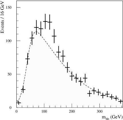
Refer to caption
Figure 24: Invariant mass for the bb¯𝑏¯𝑏b{\overline{b}} pair from the Higgs decay in the process pptt¯h𝑝𝑝𝑡¯𝑡pp\rightarrow t{\overline{t}}h at the LHC with Mh=120GeVsubscript𝑀120𝐺𝑒𝑉M_{h}=120~{}GeV (data points). The dashed line is the background. The error bars correspond to the statistical uncertainty with an integrated luminosity of L=100fb1𝐿100𝑓superscript𝑏1L=100~{}fb^{-1}.[26]

5 Heavy Top as Inspiration for Model Builders

We turn now to a discussion of the top quark in models where there is new physics involving the top quark beyond that of the Standard Model. The fact that the top quark is much heavier than the other quarks gives it a special role in electroweak symmetry breaking. In this section, we examine the role of the top quark in the minimal supersymmetric model and in models with dynamical symmetry breaking. We pay particular attention to how data from the Tevatron and the LHC can help us to test these ideas.

The large value of the top quark mass has important consequences in a supersymmetric (SUSY) model.[46] In the SM, the Higgs boson mass is a free parameter, while in a SUSY model there is an upper limit on the Higgs mass. At tree level in the minimal SUSY model, Mh<MZsubscript𝑀subscript𝑀𝑍M_{h}<M_{Z}, but the large top quark mass, and the subsequent large coupling to the Higgs boson,

mt2v1,similar-tosubscript𝑚𝑡2𝑣1{m_{t}\sqrt{2}\over v}\sim 1, (119)

lead to large radiative corrections to the prediction for the Higgs boson mass, raising the lower limit on the Higgs mass significantly. In addition, corrections due to the large top quark mass typically imply that the scalar partner of the top, the stop, is the lightest squark.

A further difference between the SM and a SUSY model which is due to the large top quark mass is the understanding of the mechanism of electroweak symmetry breaking in a SUSY model. If the supersymmetric model is embedded in a grand unified model, then the simplest version (mSUGRA) has the interesting property that the evolution of the parameters from the GUT scale to the weak scale drives the Higgs mass-squared negative as a consequence of the large value of Mtsubscript𝑀𝑡M_{t}, and therefore explains electroweak symmetry breaking. In fact, this mechanism 𝑟𝑒𝑞𝑢𝑖𝑟𝑒𝑠𝑟𝑒𝑞𝑢𝑖𝑟𝑒𝑠{\it requires} that the top quark have a mass near its observed value.

In models with dynamical symmetry breaking, the large value of the top quark mass can imply that the top quark is different from the lighter quarks, perhaps having different gauge interactions in an extended gauge sector. In Section 5.6, we discuss topcolor as an example of a model of dynamical symmetry breaking where the top quark plays a special role. Many possibilities for dynamical symmetry breaking in electroweak interactions are detailed in the review by Hill and Simmons.[47]

5.1 EWSB and the top quark mass

We begin by considering the importance of the top quark mass in the SM. In the SM, electroweak symmetry breaking occurs through the interactions of an SU(2)L𝑆𝑈subscript2𝐿SU(2)_{L} doublet scalar field, ΦΦ\Phi, with a scalar potential,[48]

Refer to caption

Figure 25: Higgs potential in the Standard Model with μ2<0superscript𝜇20\mu^{2}<0.
V=μ2ΦΦ+λ(ΦΦ)2.𝑉superscript𝜇2ΦsuperscriptΦ𝜆superscriptΦsuperscriptΦ2V=\mu^{2}\Phi\Phi^{\dagger}+\lambda(\Phi\Phi^{\dagger})^{2}~{}~{}. (120)

If μ2<0superscript𝜇20\mu^{2}<0, the neutral component of the Higgs doublet gets a vacuum expectation value,

Φ0=v2delimited-⟨⟩subscriptΦ0𝑣2\langle\Phi_{0}\rangle={v\over\sqrt{2}} (121)

and the scalar potential has the shape shown in Fig. 25. Electroweak symmetry breaking (EWSB) occurs and masses are generated for the W𝑊W and Z𝑍Z gauge bosons. After EWSB, there remains in the spectrum a physical particle, the Higgs boson, hh, and at tree level the quartic self- coupling of the Higgs boson, λ𝜆\lambda, is related to the Higgs mass by

Mh2=2λv2.superscriptsubscript𝑀22𝜆superscript𝑣2M_{h}^{2}=2\lambda v^{2}. (122)

A measurement of this relationship would test the mechanism of EWSB.

Eq. 120 is the scalar potential at the electroweak scale, Λvsimilar-toΛ𝑣\Lambda\sim v. All parameters of the electroweak theory change with the energy scale ΛΛ\Lambda in a precisely calculable way, and so will be different at higher energies. The most interesting parameters for us are the Higgs quartic self-coupling, λ𝜆\lambda, and the top quark Yukawa coupling, gtth=Mtvsubscript𝑔𝑡𝑡subscript𝑀𝑡𝑣g_{tth}={M_{t}\over v}. To one loop accuracy,444 g𝑔g and gsuperscript𝑔g^{\prime} are the SU(2)L𝑆𝑈subscript2𝐿SU(2)_{L} and U(1)Y𝑈subscript1𝑌U(1)_{Y} gauge coupling constants.

ΛdλdΛΛ𝑑𝜆𝑑Λ\displaystyle\Lambda{d\lambda\over d\Lambda} =\displaystyle= 116π2[24λ2(A12gtth2)λ+B12gtth4]116superscript𝜋2delimited-[]24superscript𝜆2𝐴12superscriptsubscript𝑔𝑡𝑡2𝜆𝐵12superscriptsubscript𝑔𝑡𝑡4\displaystyle{1\over 16\pi^{2}}\biggl{[}24\lambda^{2}-(A-12g_{tth}^{2})\lambda+B-12g_{tth}^{4}\biggr{]}
ΛdgtthdΛΛ𝑑subscript𝑔𝑡𝑡𝑑Λ\displaystyle\Lambda{dg_{tth}\over d\Lambda} =\displaystyle= 116π2(gtth12)[54gtth217g227g296gs2]116superscript𝜋2subscript𝑔𝑡𝑡12delimited-[]54superscriptsubscript𝑔𝑡𝑡217superscript𝑔227superscript𝑔296superscriptsubscript𝑔𝑠2\displaystyle{1\over 16\pi^{2}}\biggl{(}{g_{tth}\over 12}\biggr{)}\biggl{[}54g_{tth}^{2}-17g^{\prime 2}-27g^{\prime 2}-96g_{s}^{2}] (123)

where,

A𝐴\displaystyle A =\displaystyle= 3(3g2+g2)33superscript𝑔2superscript𝑔2\displaystyle 3(3g^{2}+g^{\prime 2})
B𝐵\displaystyle B =\displaystyle= 38(2g4+(g2+g2)2).382superscript𝑔4superscriptsuperscript𝑔2superscript𝑔22\displaystyle{3\over 8}\biggl{(}2g^{4}+(g^{2}+g^{\prime 2})^{2}\biggr{)}. (124)

We have omitted the equations for the running of the gauge coupling constants. They can be found in Ref. \refcitehhg.

In order for electroweak symmetry breaking to occur, the quartic coupling must remain finite at all scales,

1λ(Λ)>0.1𝜆Λ0{1\over\lambda(\Lambda)}>0. (125)

As λ𝜆\lambda is evolved from the weak scale to higher energy, it grows and eventually becomes infinite at some large scale. When λ𝜆\lambda becomes large, the scaling of Eq. 124 can be approximated,

ΛdλdΛ=32π2λ2.Λ𝑑𝜆𝑑Λ32superscript𝜋2superscript𝜆2\Lambda{d\lambda\over d\Lambda}={3\over 2\pi^{2}}\lambda^{2}~{}. (126)

Eq. 126 is easily solved,

1λ(Λ)=1λ(Mh)32π2log(ΛMh).1𝜆Λ1𝜆subscript𝑀32superscript𝜋2Λsubscript𝑀{1\over\lambda(\Lambda)}={1\over\lambda(M_{h})}-{3\over 2\pi^{2}}\log\biggl{(}{\Lambda\over M_{h}}\biggr{)}~{}. (127)

The position where λ(Λ)𝜆Λ\lambda(\Lambda)\rightarrow\infty is known as the Landau Pole. Since λ𝜆\lambda is related to the Higgs mass, Mh2=2v2λsuperscriptsubscript𝑀22superscript𝑣2𝜆M_{h}^{2}=2v^{2}\lambda, the requirement that the theory not approach the Landau pole gives an upper bound on the Higgs boson mass,

Mh2<4π2v23log(Λ/Mh).superscriptsubscript𝑀24superscript𝜋2superscript𝑣23Λsubscript𝑀M_{h}^{2}<{4\pi^{2}v^{2}\over 3\log\biggl{(}\Lambda/M_{h}\biggr{)}}~{}~{}. (128)

This means that at the scale ΛΛ\Lambda there must be some new physics beyond that of the SM which enters. The SM simply makes no sense at energy scales larger than ΛΛ\Lambda since in this region the Higgs quartic self-coupling is infinite. Assuming no new physics before the GUT scale, Λ1016GeVsimilar-toΛsuperscript1016𝐺𝑒𝑉\Lambda\sim 10^{16}~{}GeV, gives a bound on the Higgs mass of[49, 50]

Mh<160GeV.subscript𝑀160𝐺𝑒𝑉M_{h}<160~{}GeV~{}. (129)

This bound corresponds to the upper curve in Fig. 26. Non-perturbative studies using lattice gauge theory confirm the validity of this limit.[51]

Conversely, we require that the potential be bounded from below, which is equivalent to the restriction that λ>0𝜆0\lambda>0 at large ΦΦ\Phi. The scaling of the quartic coupling near λ=0𝜆0\lambda=0 is,

ΛdλdΛ=116π2[B12gtth4]Λ𝑑𝜆𝑑Λ116superscript𝜋2delimited-[]𝐵12superscriptsubscript𝑔𝑡𝑡4\Lambda{d\lambda\over d\Lambda}={1\over 16\pi^{2}}\biggl{[}B-12g_{tth}^{4}\biggr{]} (130)

which can be solved,

λ(Λ)=λ(Mh)+B12gtth416π2log(ΛMh).𝜆Λ𝜆subscript𝑀𝐵12superscriptsubscript𝑔𝑡𝑡416superscript𝜋2Λsubscript𝑀\lambda(\Lambda)=\lambda(M_{h})+{B-12g_{tth}^{4}\over 16\pi^{2}}\log\biggl{(}{\Lambda\over M_{h}}\biggr{)}~{}. (131)

The requirement that λ(Λ)>0𝜆Λ0\lambda(\Lambda)>0 gives a lower bound on the Higgs mass,

Mh22v2>12gtth4B16π2log(ΛMh).superscriptsubscript𝑀22superscript𝑣212superscriptsubscript𝑔𝑡𝑡4𝐵16superscript𝜋2Λsubscript𝑀{M_{h}^{2}\over 2v^{2}}>{12g_{tth}^{4}-B\over 16\pi^{2}}\log\biggl{(}{\Lambda\over M_{h}}\biggr{)}~{}~{}. (132)

A complete approach must include the full set of renormalization group equations, including the running of the coupling constants for large values of ΦΦ\Phi.

The restrictions on the Higgs mass from consistency of the theory are shown in Fig. 26, where the allowed region for a scale ΛΛ\Lambda is the area between the curves, known as the “chimney”. At a given scale ΛΛ\Lambda, the Higgs mass has a lower limit from bounding the potential from below and an upper limit from the requirement that Higgs quartic coupling, λ𝜆\lambda, be finite.

Refer to caption
Figure 26: Limits on the Higgs boson mass as a function of the cutoff scale ΛΛ\Lambda. The theoretically consistent region lies between the two curves.[49]

The exact shape of the allowed region depends sensitively on the value of Mtsubscript𝑀𝑡M_{t}.[49, 50]

The SM with a Higgs mass in the 130GeV130𝐺𝑒𝑉130~{}GeV region is consistent at energy scales all the way to the Planck scale. The theory is still unsatisfactory however, because it provides no explanation of why μ2<0superscript𝜇20\mu^{2}<0, as required for EWSB. In addition, the Higgs mass is a free parameter in the SM and there is no understanding of why it should have any particular value. In the next section, we will see that low energy supersymmetry can potentially solve both these problems.

5.2 Supersymmetry and the Top Quark

TeV scale supersymmetric models explain several mysteries about the SM:

  • A heavy top quark and mSUGRA (minimal supergravity) explain why μ2<0superscript𝜇20\mu^{2}<0.

  • A heavy top quark and the MSSM (minimal supersymmetric Standard Model) explain why the Higgs mass may light, as suggested by precision measurements.

In this section, we give a brief review of phenomenological models of supersymmetry and discuss the relationship between the top quark mass and the requirement that supersymmetry exist below the TeV scale.

Supersymmetry is a symmetry which relates the masses and couplings of particles of differing spin. To each SM chiral fermion is associated a complex scalar and each of the SU(3)×SU(2)L×U(1)Y𝑆𝑈3𝑆𝑈subscript2𝐿𝑈subscript1𝑌SU(3)\times SU(2)_{L}\times U(1)_{Y} gauge bosons similarly acquires a Majorana fermion partner. Supersymmetry connects particles of differing spin, but with all other characteristics the same.[52] In an unbroken supersymmetric model, particles and their superpartners have identical masses. It is clear, then, that supersymmetry must be a broken symmetry if it is to be a theory of low energy interactions. There is no scalar particle, for example, with the mass and quantum numbers of the electron. In fact, there are no candidate supersymmetric scalar partners for any of the fermions in the experimentally observed spectrum. The most general soft breaking of supersymmetry introduces masses and mixing parameters and the theory loses much of its capabilities for specific predictions.

The Higgs sector in a SUSY model always contains at least two SU(2)L𝑆𝑈subscript2𝐿SU(2)_{L} doublets. In the supersymmetric extension of the Standard Model, the Higgs doublet acquires a SUSY partner which is an SU(2)L𝑆𝑈subscript2𝐿SU(2)_{L} doublet of Majorana fermion fields, h~1subscript~1{\tilde{h}}_{1} (the Higgsinos), which contribute to the triangle SU(2)L𝑆𝑈subscript2𝐿SU(2)_{L} and U(1)Y𝑈subscript1𝑌U(1)_{Y} gauge anomalies as described in Section 2.1. Since the fermions of the Standard Model have exactly the right quantum numbers to cancel these anomalies, it follows that the contribution from the fermionic partner of the Higgs doublet remains uncancelled.[6, 7] This contribution must be cancelled by adding a second Higgs doublet (and its Majorana fermion partner) with precisely the opposite U(1)Y𝑈subscript1𝑌U(1)_{Y} quantum numbers from the first Higgs doublet.

All supersymmetric models thus have at least 2-Higgs doublets and so the minimal supersymmetric model has 5 physical Higgs bosons: h0,H0,A0,H±superscript0superscript𝐻0superscript𝐴0superscript𝐻plus-or-minush^{0},H^{0},A^{0},H^{\pm}. The ratio of the vacuum expectation values of the neutral Higgs bosons,

tanβv2v1𝛽subscript𝑣2subscript𝑣1\tan\beta\equiv{v_{2}\over v_{1}} (133)

is a fundamental parameter of the theory. At tree level, the neutral Higgs boson masses are predicted in terms of two parameters, which are usually taken to be tanβ𝛽\tan\beta and the mass of the pseudoscalar Higgs boson, MAsubscript𝑀𝐴M_{A}. The neutral Higgs boson masses are then predicted,

Mh,H2=12(MA2+MZ2)12(MA2+MZ2)24MZ2MA2cos22βsuperscriptsubscript𝑀𝐻2minus-or-plus12superscriptsubscript𝑀𝐴2superscriptsubscript𝑀𝑍212superscriptsuperscriptsubscript𝑀𝐴2superscriptsubscript𝑀𝑍224superscriptsubscript𝑀𝑍2superscriptsubscript𝑀𝐴2superscript22𝛽M_{h,H}^{2}={1\over 2}(M_{A}^{2}+M_{Z}^{2})\mp{1\over 2}\sqrt{(M_{A}^{2}+M_{Z}^{2})^{2}-4M_{Z}^{2}M_{A}^{2}\cos^{2}2\beta} (134)

which gives an upper bound on the lightest Higgs mass:

Mh<MZcos2β<MZsubscript𝑀subscript𝑀𝑍delimited-∣∣2𝛽subscript𝑀𝑍M_{h}<M_{Z}\mid\cos 2\beta\mid<M_{Z} (135)

which is excluded experimentally. (In a SUSY model, the LEP and LEPII results require Mh>89.8GeVsubscript𝑀89.8𝐺𝑒𝑉M_{h}>89.8~{}GeV.[4])

The Higgs mass prediction in a supersymmetric model receives large radiative corrections from top and stop squark loops. At 1-loop, and neglecting possible soft SUSY breaking tri-linear scalar mixing, the lightest Higgs mass becomes:

Mh2superscriptsubscript𝑀2\displaystyle M_{h}^{2} =\displaystyle= MA2+MZ2+ϵ212{(MA2+MZ2+ϵ)24MZ2MA2cos22β\displaystyle{M_{A}^{2}+M_{Z}^{2}+\epsilon\over 2}-{1\over 2}\biggl{\{}(M_{A}^{2}+M_{Z}^{2}+\epsilon)^{2}-4M_{Z}^{2}M_{A}^{2}\cos^{2}2\beta (136)
4ϵ(MA2sin2β+MZ2cos2β)}1/2\displaystyle-4\epsilon(M_{A}^{2}\sin^{2}\beta+M_{Z}^{2}\cos^{2}\beta)\biggr{\}}^{1/2}

where,

ϵ=italic-ϵabsent\displaystyle\epsilon= 3GF2π2Mt4sin2βlog(M~t2Mt2),3subscript𝐺𝐹2superscript𝜋2superscriptsubscript𝑀𝑡4superscript2𝛽superscriptsubscript~𝑀𝑡2superscriptsubscript𝑀𝑡2\displaystyle{3G_{F}\over\sqrt{2}\pi^{2}}{M_{t}^{4}\over\sin^{2}\beta}\log\biggl{(}{{\tilde{M}}_{t}^{2}\over M_{t}^{2}}\biggr{)}, (137)

and M~tsubscript~𝑀𝑡{\tilde{M}}_{t} is the average stop squark mass. For unbroken supersymmetry, the top and stop have the same masses, Mt=M~tsubscript𝑀𝑡subscript~𝑀𝑡M_{t}={\tilde{M}}_{t}, and the bound of Eq. 135 is recovered. The mass splitting between the top and stop in a broken SUSY theory changes the upper bound on the Higgs mass to,

Mh2<MZ2cos22β+ϵsin2β.superscriptsubscript𝑀2superscriptsubscript𝑀𝑍2superscript22𝛽italic-ϵsuperscript2𝛽M_{h}^{2}<M_{Z}^{2}\cos^{2}2\beta+\epsilon\sin^{2}\beta. (138)

The large Mt4superscriptsubscript𝑀𝑡4M_{t}^{4} corrections raise the Higgs mass bound above the experimental limit, as shown in Fig. 27.

Refer to caption
Figure 27: Upper bound on Higgs mass in MSSM at one loop and with no soft trilinear mixing.[53]

There are many analyses[53] which include a variety of two-loop effects, renormalization group effects, etc., but the important point is that for given values of tanβ𝛽\tan\beta, the scalar mixing parameters, and the squark masses, there is an upper bound on the lightest neutral Higgs boson mass. For large values of tanβ𝛽\tan\beta the limit is relatively insensitive to the value of tanβ𝛽\tan\beta and with a squark mass less than about 1TeV1𝑇𝑒𝑉1~{}TeV, the upper limit on the Higgs mass is about 110GeV110𝐺𝑒𝑉110~{}GeV if mixing in the top squark sector is negligible. For large mixing, this limit is raised to around 130GeV130𝐺𝑒𝑉130~{}GeV.

5.3 mSUGRA

The minimal supersymmetric model (MSSM) is constructed by adding to the Lagrangian all of the soft supersymmetry breaking terms allowed by the gauge symmetries. These include masses for all the new SUSY particles and tri-linear scalar mixing terms. The most general Lagrangian of this type has 105 new parameters beyond those of the Standard Model. In order to make definite predictions, the simplifying assumption that the soft parameters unify at MGUTsubscript𝑀𝐺𝑈𝑇M_{GUT} is often made. (The resulting model is usually called mSUGRA or the CMSSM). In this framework the model is completely specified by five parameters:

  • Common scalar mass at MGUTsubscript𝑀𝐺𝑈𝑇M_{GUT}, m~0subscript~𝑚0{\tilde{m}}_{0}

  • Common gaugino mass at MGUTsubscript𝑀𝐺𝑈𝑇M_{GUT}, M1/2subscript𝑀12M_{1/2}

  • 1 Higgs mass-squared, m122superscriptsubscript𝑚122m_{12}^{2}

  • 1 tri-linear coupling at MGUTsubscript𝑀𝐺𝑈𝑇M_{GUT}, A0λFsubscript𝐴0subscript𝜆𝐹A_{0}\lambda_{F}

  • sign(μ^)^𝜇({\hat{\mu}})

The parameter μ^^𝜇{\hat{\mu}} describes the mixing between the two Higgs doublets. At the GUT scale, the Higgs masses are,

Mh,H2(MGUT)=m02+μ^2,superscriptsubscript𝑀𝐻2subscript𝑀𝐺𝑈𝑇superscriptsubscript𝑚02superscript^𝜇2M_{h,H}^{2}(M_{GUT})=m_{0}^{2}+{\hat{\mu}}^{2}, (139)

while the squark and slepton masses are

Mq~2(MGUT)=Ml~2(MGUT)=m02.superscriptsubscript𝑀~𝑞2subscript𝑀𝐺𝑈𝑇superscriptsubscript𝑀~𝑙2subscript𝑀𝐺𝑈𝑇superscriptsubscript𝑚02M_{\tilde{q}}^{2}(M_{GUT})=M_{\tilde{l}}^{2}(M_{GUT})=m_{0}^{2}~{}. (140)

The theory must explain why the lightest neutral Higgs mass-squared becomes negative at the weak scale and breaks the electroweak symmetry, while the scalar fermion masses remain positive so as to not break color and electromagnetism.

In an mSUGRA model, the masses and parameters are evolved using the renormalization group equations (RGE) to scale from MGUTsubscript𝑀𝐺𝑈𝑇M_{GUT} down to the weak scale in order to make predictions for the masses at the weak scale. The large top quark mass plays an important role here. We can understand the basic scaling by considering only the Higgs doublet, H2subscript𝐻2H_{2},555H2subscript𝐻2H_{2} is the SU(2)L𝑆𝑈subscript2𝐿SU(2)_{L} doublet with isospin Y=+12𝑌12Y=+{1\over 2}. the scalar partners of the third generation SU(2)L𝑆𝑈subscript2𝐿SU(2)_{L} fermion doublet, (t~L,b~L)Q~3subscript~𝑡𝐿subscript~𝑏𝐿subscript~𝑄3({\tilde{t}}_{L},{\tilde{b}}_{L})\equiv{\tilde{Q}}_{3}, and the scalar partner of the right-handed top quark, t~Rsubscript~𝑡𝑅{\tilde{t}}_{R}. The renormalization group scaling is given by:[54]

dMH22dlog(Λ)𝑑superscriptsubscript𝑀subscript𝐻22𝑑Λ\displaystyle{dM_{H_{2}}^{2}\over d\log(\Lambda)} =\displaystyle= 18π2(3gtth2Xt3g2M22g2M12)18superscript𝜋23superscriptsubscript𝑔𝑡𝑡2subscript𝑋𝑡3superscript𝑔2superscriptsubscript𝑀22superscript𝑔2superscriptsubscript𝑀12\displaystyle{1\over 8\pi^{2}}(3g_{tth}^{2}X_{t}-3g^{2}M_{2}^{2}-g^{\prime 2}M_{1}^{2})
dM~tR2dlog(Λ)𝑑superscriptsubscript~𝑀subscript𝑡𝑅2𝑑Λ\displaystyle{d{\tilde{M}}_{t_{R}}^{2}\over d\log(\Lambda)} =\displaystyle= 18π2(2gtth2Xt163gs2M32169g2M12)18superscript𝜋22superscriptsubscript𝑔𝑡𝑡2subscript𝑋𝑡163superscriptsubscript𝑔𝑠2superscriptsubscript𝑀32169superscript𝑔2superscriptsubscript𝑀12\displaystyle{1\over 8\pi^{2}}(2g_{tth}^{2}X_{t}-{16\over 3}g_{s}^{2}M_{3}^{2}-{16\over 9}g^{\prime 2}M_{1}^{2})
dM~Q32dlog(Λ)𝑑superscriptsubscript~𝑀subscript𝑄32𝑑Λ\displaystyle{d{\tilde{M}}_{Q_{3}}^{2}\over d\log(\Lambda)} =\displaystyle= 18π2(gtth2Xt163gs2M323g2M2219g2M12)18superscript𝜋2superscriptsubscript𝑔𝑡𝑡2subscript𝑋𝑡163superscriptsubscript𝑔𝑠2superscriptsubscript𝑀323superscript𝑔2superscriptsubscript𝑀2219superscript𝑔2superscriptsubscript𝑀12\displaystyle{1\over 8\pi^{2}}(g_{tth}^{2}X_{t}-{16\over 3}g_{s}^{2}M_{3}^{2}-3g^{2}M_{2}^{2}-{1\over 9}g^{\prime 2}M_{1}^{2})

where,

Xtsubscript𝑋𝑡\displaystyle X_{t} \displaystyle\equiv MH22+M~Q32+M~tR2+At2.subscriptsuperscript𝑀2subscript𝐻2subscriptsuperscript~𝑀2subscript𝑄3subscriptsuperscript~𝑀2subscript𝑡𝑅superscriptsubscript𝐴𝑡2\displaystyle M^{2}_{H_{2}}+{\tilde{M}}^{2}_{Q_{3}}+{\tilde{M}}^{2}_{{t_{R}}}+A_{t}^{2}~{}. (141)

M3,2,1subscript𝑀321M_{3,2,1} are the gaugino masses associated with the SU(3)×SU(2)L×U(1)Y𝑆𝑈3𝑆𝑈subscript2𝐿𝑈subscript1𝑌SU(3)\times SU(2)_{L}\times U(1)_{Y} gauge sector, gtthsubscript𝑔𝑡𝑡g_{tth} is the coupling of the Higgs to the top quark in the MSSM, and Atsubscript𝐴𝑡A_{t} is the soft SUSY mixing term in the top sector. The QCD term (proportional to gs2superscriptsubscript𝑔𝑠2g_{s}^{2}) makes M~tR2,M~Q32superscriptsubscript~𝑀subscript𝑡𝑅2superscriptsubscript~𝑀subscript𝑄32{\tilde{M}}_{t_{R}}^{2},{\tilde{M}}_{Q_{3}}^{2} increase faster than MH2subscript𝑀subscript𝐻2M_{H_{2}} as the scale is reduced from MGUTsubscript𝑀𝐺𝑈𝑇M_{GUT}. The Yukawa term (proportional to gtthsubscript𝑔𝑡𝑡g_{tth}) drives MH22<0superscriptsubscript𝑀subscript𝐻220M_{H_{2}}^{2}<0, while the other scalar mass-squared terms remain positive. This behavior is a consequence of the large Mtsubscript𝑀𝑡M_{t} value.

Neglecting the gauge couplings, we have:

ddlog(Λ)(MH22M~tR2M~Q32)=gtth28π2Xt(321),𝑑𝑑Λmatrixsuperscriptsubscript𝑀subscript𝐻22superscriptsubscript~𝑀𝑡𝑅2superscriptsubscript~𝑀subscript𝑄32superscriptsubscript𝑔𝑡𝑡28superscript𝜋2subscript𝑋𝑡matrix321{d\over d\log(\Lambda)}\left(\begin{matrix}M_{H_{2}}^{2}\cr{\tilde{M}}_{tR}^{2}\cr{\tilde{M}}_{Q_{3}}^{2}\cr\end{matrix}\right)={g_{tth}^{2}\over 8\pi^{2}}X_{t}\left(\begin{matrix}3\cr 2\cr 1\cr\end{matrix}\right)~{}, (142)

which can be easily solved,

Mh2(Λ)=Mh2(MGUT)3gtth28π2Xtlog(MGUTΛ).superscriptsubscript𝑀2Λsuperscriptsubscript𝑀2subscript𝑀𝐺𝑈𝑇3superscriptsubscript𝑔𝑡𝑡28superscript𝜋2subscript𝑋𝑡subscript𝑀𝐺𝑈𝑇ΛM_{h}^{2}(\Lambda)=M_{h}^{2}(M_{GUT})-{3g_{tth}^{2}\over 8\pi^{2}}X_{t}\log({M_{GUT}\over\Lambda})~{}. (143)

For heavy Mtsubscript𝑀𝑡M_{t}, Mh2superscriptsubscript𝑀2M_{h}^{2} becomes negative and triggers EWSB. It is interesting that this behavior 𝑟𝑒𝑞𝑢𝑖𝑟𝑒𝑠𝑟𝑒𝑞𝑢𝑖𝑟𝑒𝑠{\it requires} Mt175GeVsimilar-tosubscript𝑀𝑡175𝐺𝑒𝑉M_{t}\sim 175~{}GeV.[55]

The RGE scaling from the GUT scale to the weak scale in mSUGRA type models yields a a typical pattern of masses, as seen in Fig. 28. The gluino is the heaviest gaugino, while the squarks are significantly heavier than the sleptons.
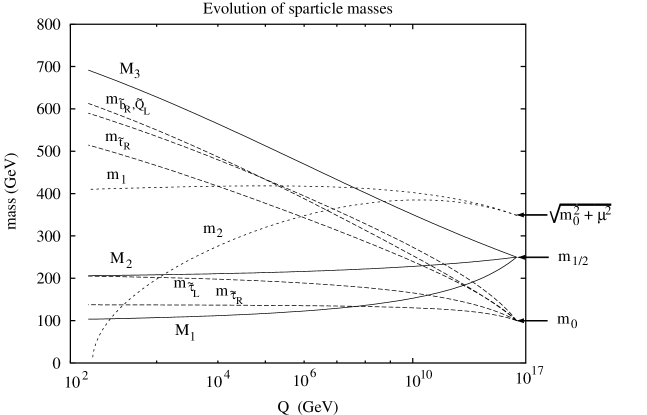
Refer to caption

Figure 28: Typical pattern of masses in an mSUGRA model.[55].

5.4 Charged Higgs Decays

The pattern of top quark decays is changed in the MSSM from that of the SM, due to the extended Higgs sector. The presence of a charged Higgs boson allows the decay, tH+b𝑡superscript𝐻𝑏t\rightarrow H^{+}b if the mass of the charged Higgs is less than Mtmbsubscript𝑀𝑡subscript𝑚𝑏M_{t}-m_{b}. This decay looks similar to tWb𝑡𝑊𝑏t\rightarrow Wb and can have a significant rate. The coupling of the charged Higgs to the tb𝑡𝑏t~{}b system is,

gtH+bmtcotβP++mbtanβPsimilar-tosubscript𝑔𝑡superscript𝐻𝑏subscript𝑚𝑡𝛽subscript𝑃subscript𝑚𝑏𝛽subscript𝑃g_{tH^{+}b}\sim m_{t}\cot\beta P_{+}+m_{b}\tan\beta P_{-} (144)

and so this decay is relevant both for very large and for very small tanβ𝛽\tan\beta. For small tanβ𝛽\tan\beta, H+cssuperscript𝐻𝑐𝑠H^{+}\rightarrow cs and H+tbsuperscript𝐻superscript𝑡𝑏H^{+}\rightarrow t^{*}b, while for large tanβ𝛽\tan\beta, H+τνsuperscript𝐻𝜏𝜈H^{+}\rightarrow\tau\nu. These decays would suppress the rate for top decays to leptons plus jets in the SM top search. In Run I, the Tevatron experiments placed a limit on MH+subscript𝑀superscript𝐻M_{H^{+}} of roughly MH+>100GeVsubscript𝑀superscript𝐻100𝐺𝑒𝑉M_{H^{+}}>100~{}GeV for tanβ<1𝛽1\tan\beta<1 or tanβ>50𝛽50\tan\beta>50.[56]

5.5 The Top squark

The mass-squared matrix for the scalar partners of the left and right handed top quarks (t~L,t~Rsubscript~𝑡𝐿subscript~𝑡𝑅{\tilde{t}}_{L},{\tilde{t}}_{R}) includes mixing between the partners of the left- and right- handed top:

M~t2=(M~Q32+Mt2Mt(Atμ^cotβ)+MZ2Ltcos2βM~tR2+Mt2Mt(Atμ^cotβ)+MZ2Rtcos2β)superscriptsubscript~𝑀𝑡2matrixsuperscriptsubscript~𝑀subscript𝑄32superscriptsubscript𝑀𝑡2subscript𝑀𝑡subscript𝐴𝑡^𝜇𝛽superscriptsubscript𝑀𝑍2subscript𝐿𝑡2𝛽missing-subexpressionmissing-subexpressionsuperscriptsubscript~𝑀subscript𝑡𝑅2superscriptsubscript𝑀𝑡2subscript𝑀𝑡subscript𝐴𝑡^𝜇𝛽superscriptsubscript𝑀𝑍2subscript𝑅𝑡2𝛽{\tilde{M}}_{t}^{2}=\left(\begin{matrix}{\tilde{M}}_{Q_{3}}^{2}+M_{t}^{2}&M_{t}(A_{t}-{\hat{\mu}}\cot\beta)\cr~{}~{}~{}+M_{Z}^{2}L_{t}\cos 2\beta&\cr&{\tilde{M}}_{t_{R}}^{2}+M_{t}^{2}\cr M_{t}(A_{t}-{\hat{\mu}}\cot\beta)&~{}~{}~{}+M_{Z}^{2}R_{t}\cos 2\beta\cr\end{matrix}\right)

The mixing is proportional to the top quark mass and so the large value of Mtsubscript𝑀𝑡M_{t} can cause one of the top squarks to be relatively light. If the scalar mass scale, M~Q3subscript~𝑀subscript𝑄3{\tilde{M}}_{Q_{3}} is much larger than MZ,Mt,Atsubscript𝑀𝑍subscript𝑀𝑡subscript𝐴𝑡M_{Z},M_{t},A_{t}, then the stop masses are roughly degenerate M~Q3similar-toabsentsubscript~𝑀subscript𝑄3\sim{\tilde{M}}_{Q_{3}}. On the other hand if M~Q3MZ,Mt,Atsimilar-tosubscript~𝑀subscript𝑄3subscript𝑀𝑍subscript𝑀𝑡subscript𝐴𝑡{\tilde{M}}_{Q_{3}}\sim M_{Z},M_{t},A_{t}, then the large mixing effects drive the stop mass to a small value and the stop squark becomes the lightest squark.

It is possible to search for a light stop in the decays of the top, tt~χ~0𝑡~𝑡superscript~𝜒0t\rightarrow{\tilde{t}}{\tilde{\chi}}^{0}, where χ~0superscript~𝜒0{\tilde{\chi}}^{0} is the lightest neutral SUSY particle. The limits then depend on the assumed branching ratio for the top into stop decays. The Run I data was sensitive to stop and chargino masses in the 100GeV100𝐺𝑒𝑉100~{}GeV range.[57]

5.6 The Top Quark and Dynamical Symmetry Breaking

The top quark has a special role in technicolor models where a tt¯𝑡¯𝑡t{\overline{t}} condensate can play the part of the Higgs boson in generating EWSB. This can happen in models where there is a new strong interaction felt by the top quark, but not by the lighter quarks. The proto-type model of this type is called 𝑡𝑜𝑝𝑐𝑜𝑙𝑜𝑟𝑡𝑜𝑝𝑐𝑜𝑙𝑜𝑟{\it topcolor}.[topref] A review of this class of models can be found in Ref. [47]. Topcolor models are constructed by expanding the strong gauge group from the SU(3)𝑆𝑈3SU(3) of QCD to,

SU(3)tc×SU(3)SU(3)QCD𝑆𝑈subscript3𝑡𝑐𝑆𝑈3𝑆𝑈subscript3𝑄𝐶𝐷SU(3)_{tc}\times SU(3)\rightarrow SU(3)_{QCD} (145)

SU(3)tc𝑆𝑈subscript3𝑡𝑐SU(3)_{tc} couples only to the 3rd generation with a coupling gtcsubscript𝑔𝑡𝑐g_{tc}, while the second SU(3)𝑆𝑈3SU(3) gauge symmetry couples only to the first two generations. The symmetry is broken to SU(3)QCD𝑆𝑈subscript3𝑄𝐶𝐷SU(3)_{QCD} at a scale M𝑀M. Below M𝑀M, the gauge bosons of the SU(3)tc𝑆𝑈subscript3𝑡𝑐SU(3)_{tc} group, the “topgluons”, are massive and lead to effective 4-Fermi interactions between the top quarks:

Lgtc2M2(Q¯3LγμTA2Q3L)(t¯RγμTA2tR),similar-to𝐿superscriptsubscript𝑔𝑡𝑐2superscript𝑀2subscript¯𝑄3𝐿subscript𝛾𝜇superscript𝑇𝐴2subscript𝑄3𝐿subscript¯𝑡𝑅superscript𝛾𝜇superscript𝑇𝐴2subscript𝑡𝑅{\it L}\sim{g_{tc}^{2}\over M^{2}}({\overline{Q}}_{3L}\gamma_{\mu}{T^{A}\over 2}Q_{3L})({\overline{t}}_{R}\gamma^{\mu}{T^{A}\over 2}t_{R}), (146)

where TAsuperscript𝑇𝐴T^{A} is the SU(3)𝑆𝑈3SU(3) generator in the adjoint representation and Q3Lsubscript𝑄3𝐿Q_{3L} is the left-handed (tL,bL)subscript𝑡𝐿subscript𝑏𝐿(t_{L},b_{L}) doublet. If the SU(3)tc𝑆𝑈subscript3𝑡𝑐SU(3)_{tc} coupling, gtcsubscript𝑔𝑡𝑐g_{tc}, is larger than a critical value, a top condensate forms, t¯tdelimited-⟨⟩¯𝑡𝑡\langle{\overline{t}}t\rangle, which breaks the electroweak symmetry and generates a mass for the top quark. One must arrange that t¯t0delimited-⟨⟩¯𝑡𝑡0\langle{\overline{t}}t\rangle\neq 0 and b¯b=0delimited-⟨⟩¯𝑏𝑏0\langle{\overline{b}}b\rangle=0. This is usually done by adding an additional U(1)h𝑈subscript1U(1)_{h} gauge symmetry under which the t𝑡t and b𝑏b quarks transform differently.

This class of models can be tested at the Tevatron and the LHC by searching for effects of the top gluons and the new Zsuperscript𝑍Z^{\prime}, and through B𝐵B decays.[59] Since the Zsuperscript𝑍Z^{\prime} boson corresponding to the U(1)h𝑈subscript1U(1)_{h} and the top gluons of SU(3)tc𝑆𝑈subscript3𝑡𝑐SU(3)_{tc} couple differently to the third generation and to the lighter quarks, they lead to flavor changing neutral currents. Present limits from B𝐵B meson mixing require that the topgluon be heavier than 35TeV35𝑇𝑒𝑉3-5~{}TeV and MZ>710GeVsubscript𝑀superscript𝑍710𝐺𝑒𝑉M_{Z^{\prime}}>7-10~{}GeV.[58]

6 Conclusions

The story of the top quark is far from over. Its properties and its role in the SM and in physics beyond the SM will be further elucidated in the emerging Run II data at the Tevatron. The increased statistics of Run II will enable more precise measurements of the mass, couplings, and decay properties of the top. The LHC will provide even more insight into the role of the top quark. It is possible that surprises are just around the corner!

Acknowledgements

I would like to thank K.T. Mohanthapa, H. Haber, and A. Nelson for organizing such an enjoyable and successful school.

References

  • [1] T. Abe . et. al., Phys. Rev. Lett. 74 (1995) 2626, Phys. Rev. D50 (1994) 2966; S. Abachi et. al., Phys. Rev. Lett. 74 (1995) 2632, hep-ex/9503003.
  • [2] F. Abe et. al., Phys. Rev. Lett. 82 (1999) 271, hep-ex/9810029; S. Abachi et. al., Phys. Rev. D60 (1999) 052001.
  • [3] See results of LEP Electroweak Working Group, http://lepewwg.web.cern.ch/LEPEWWG/.
  • [4] Particle Data Group, K. Hagiwara et. al., Phys. Rev. D66 (2002) 010001.
  • [5] E. Simmons, TASI2000, hep-ph/0011244; S. Willenbrock, Rev. Mod. Phys. 72 (2000) 1141, hep-ph/0211067; hep-ph/0008189.
  • [6] M. Peskin and D.Schroeder, An Introduction  to  Quantum  Field  Theory, (Addison-Wesley, Reading, 1995).
  • [7] C. Quigg, Gauge  Theories  of  the  Strong,  Weak,  and  Electromagnetic  Interactions, (Benjamin-Cummings, Reading, 1983).
  • [8] E. Rice et. al., Phys. Rev. Lett. 48 (1982) 906.
  • [9] J. Kuhn, The Top Quark and  The  Electroweak Interaction, 1995 SLAC Summer School, hep-ph/9707321.
  • [10] G. Degrassi and A. Sirlin, Nucl. Phys. B352 (1991) 342.
  • [11] M. Carena et. al., Report of the Tevatron Higgs Working Group, hep-ph/0010338.
  • [12] P. Nason, S. Dawson, and R. K. Ellis, Nucl. Phys. B303 (1988) 607.
  • [13] W. Beenakker, H. Huijf, W. van Neerven, and J. Smith, Phys. Rev. D40 (1989) 54.
  • [14] S. Catani et. al., Phys. Lett. B378 (1996) 329, hep-ph/9602208; E. Berger and H. Contopanagos, Phys. Lett. B361 (1995) 115, hep-ph/9507363; E. Laenen, J. Smith, and W. van Neerven, Nucl. Phys. B369 (1992) 543; R. Bonciani, S. Catani, M. Mangano, and P. Nason, Nucl. Phys. B529 (1998) 424, hep-ph/9801375.
  • [15] M. Cacciari et. al., hep-ph/0303085.
  • [16] F.  Abe et. al., Phys. Rev. Lett. 80 (1998) 2773, hep-ph/971008; S. Abachi et. al., Phys. Rev. Lett. 79 (1997) 1203; hep-ex/9703008.
  • [17] T. Affolder 𝑒𝑡.𝑎𝑙.formulae-sequence𝑒𝑡𝑎𝑙{\it et.al.}, Phys. Rev. Lett. 86 (2001) 3233, hep-ph/0012029.
  • [18] G. Eilam et.al., Phys. Rev. Lett., 66 (1991) 3105; T. Mehen, Phys. Lett. B417 (1998) 353, hep-ph/9707365.
  • [19] T. Affolder et. al., Phys. Rev. Lett. 84 (2000) 216, hep-ph/9909042.
  • [20] D. Amidei and R. Brock, Tev 2000 Study (1996), FERMILAB-Pub-96/082.
  • [21] J. Womersley, TASI02, Boulder, Colorado, hep-ex/0301007; D. Chakraborty, J. Konigsberg, and D. Rainwater, hep-ph/0303092.
  • [22] F. Abe et. al., Phys. Rev. Lett. 80 (1998) 2767, hep-ex/9801014; S. Abachi et. al., Phys. Rev. Lett. 79 (1997) 1197, hep-ex/9703008.
  • [23] M. Smith and W. Willenbrock, Phys. Rev. D54 (1996) 6696, hep-ph/9604223; S. Zhu, Phys. Lett. B524 (2002) 238, hep-ph/0109269.
  • [24] T. Stelzer, Z. Sullivan, and S. Willenbrock, Phys. Rev. D56 (1997) 5919, hep-ph/9705398.
  • [25] U. Baur et. al., Snowmass 2001, Snowmass, Colorado, hep-ph/0202001.
  • [26] M. Beneke et. al., LHC Top Study, hep-ph/0003033.
  • [27] G. Mahlon and S. Parke, Phys. Lett. B411 (1997) 173, hep-ph/9706304; V. Barger, J. Ohnemus, and R. Phillips, Int. J. Mod. Phys. A4 (1989) 617.
  • [28] J. Jersak, E. Laermann and P. Zerwas, Phys. Rev. D25 (1982) 1218; V. Ravindran and W. van Neerven, Phys. Lett. B445 (1998) 214, hep-ph/9809411.
  • [29] H. Baer, J. Ohnemus, and J. Owens, Phys. Rev D40 (1989) 2844.
  • [30] B. Harris and J. Owens, Phys. Rev. D65 (094032) , hep-ph/0102128.
  • [31] W. Giele and N. Glover, Phys. Rev. D46 (1992) 1980; W. Giele, N. Glover, and D. Kosower, Nucl. Phys. B403 (1993) 633, hep-ph/9302225.
  • [32] G. Sterman, Introduction  to  Quantum Field Theory (Cambridge University Press, Cambridge, 1993).
  • [33] G. Grammer and D. Yennie, Phys. Rev. D8 (1973) 4332; F. Fiorani, G. Marchesini, and L. Reina, Nucl. Phys. B309 (1988) 439.
  • [34] L. Reina, S. Dawson, and D.  Wackeroth, Phys. Rev. D65 (2002) 053017, hep-ph/0109066.
  • [35] Y. Sumino et.al., Phys. Rev. D47 (1993) 56.
  • [36] A. Hoang, A. Manohar, and I. Stewart, Phys. Rev. D65 (2002) 014014, hep-ph/0107144.
  • [37] S. Groote and O. Yakovlev, Phys. Rev. D63 (2001) 074012, hep-ph/0008156.
  • [38] A. Hoang and T. Teubner, Phys. Rev. D60 (1999) 114027, hep-ph/9904468.
  • [39] S. Dawson and L. Reina, Phys. Rev. D59 (1999) 054012, hep-ph/9808443.
  • [40] S.  Dittmaier et al, Phys. Lett. B441 (1998)383, hep-ph/9808433.
  • [41] A. Juste and G. Merino, hep-ph/9910301; A. Gay, www.desy.de/ desch/higgs/stmalo/gay.ps.
  • [42] H. Baer, S. Dawson, and L. Reina, Phys. Rev. D61 (2000) 013002, hep-ph/9906419.
  • [43] L. Reina and S. Dawson, Phys. Rev. Lett. 87 (2001) 201804, hep-ph/0107101; S. Dawson, L. Orr, L. Reina, and D. Wackeroth, hep-ph/0211438; W. Beenakker et. al., Nucl. Phys. B653 (2003) 151, hep-ph/0211352; W. Beenakker et. al., Phys. Rev. Lett. 87 (2001) 201805, hep-ph/0107-81.
  • [44] G. van Oldenborgh and J. Vermaseren, Z. Phys. C46 (1990) 425.
  • [45] U. Baur, S. Keller, and D. Wackeroth, Phys. Rev. D59 (1999) 013002, hep-ph/9807417.
  • [46] J. Bagger, TASI95, hep-ph/9604232, M. Dine, TASI96, hep-ph/9612389, S. Martin, in Perspectives  on  Supersymmetry, ed. G. Kane (World Scientific, Singapore, 1998) hep-ph/9709356, S. Dawson, TASI97,hep-ph/9712464
  • [47] C. Hill and E. Simmons, hep-ph/0203079.
  • [48] J.  Gunion et. al., The Higgs Hunters Guide, (Addison-Wesley, Menlo Park, 1990).
  • [49] M. Sher, Phys. Rep. 179 (1989) 273.
  • [50] J. Casas, J. Espinosa, and M.  Quiros, Phys. Lett. B342 (1995) 171, hep-ph/9409458; B382 (1996) 374, hep-ph/9603227.
  • [51] M. Luscher and P. Weisz, Nucl. Phys. B318 (1989) 705; A. Hasenfratz et. al., Nucl. Phys. B317 (1989) 81.
  • [52] J. Wess and J.  Bagger, Supersymmetry and Supergravity, (Princeton University Press, Princeton, 1983).
  • [53] M. Carena et al, Nucl. Phys. B580 (2000) 29, hep-ph/0001002; R. J. Zhang, Phys. Lett. B447 (1999) 89, hep-ph/9808299; R. Hempfling and H. Hoang, Phys. Lett. B331 (1994) 99, hep-ph/9401219; S. Heinemeyer, W. Hollik, and G. Weiglein, Phys. Rev. D58 (1998) 091701, hep-ph/9803277.
  • [54] M. Machacek and M. Vaughn, Nucl. Phys. B222 (1983) 83; C. Ford et. al., Nucl. Phys. B395 (1993) 17.
  • [55] V. Barger, M. Berger, and P. Ohmann, Phys. Rev. D49 (1994) 4908, hep-ph/9311269.
  • [56] B. Abbott et. al., Phys. Rev. Lett. 82 (1999) 4975, hep-ex/9902028; R. Demina et. al., Phys. Rev. D62 (2000) 035011, hep-ex/9910275.
  • [57] T. Affolder, Phys. Rev. Lett. 84 (2000)5704, hep-ex/9910049; Phys. Rev. Lett. 84 (2000) 5273, hep-ex/9912018.
  • [58] G. Burdman, K. Land, and T. Rador, Phys. Lett. B514 (2001) 41, hep-ph/0012073.
  • [59] E. Simmons, hep-ph/0211335.