IRB$-$TH$-$2/03

Reduction method for dimensionally regulated one-loop N-point Feynman integrals
G. Duplančić and B. Nižić

Theoretical Physics Division, Rudjer Bošković Institute, P.O. Box 180, HR-10002 Zagreb, Croatia

We present a systematic method for reducing an arbitrary one$-$loop $N-$point massless Feynman integral with generic 4$-$dimensional momenta to a set comprised of eight fundamental scalar integrals: six box integrals in $D=6$, a triangle integral in $D=4$, and a general two$-$point integral in $D$ space time dimensions. All the divergences present in the original integral are contained in the general two$-$point integral and associated coefficients. The problem of vanishing of the kinematic determinants has been solved in an elegant and transparent manner. Being derived with no restrictions regarding the external momenta, the method is completely general and applicable for arbitrary kinematics. In particular, it applies to the integrals in which the set of external momenta contains subsets comprised of two or more collinear momenta, which are unavoidable when calculating one$-$loop contributions to the hard$-$scattering amplitude for exclusive hadronic processes at large momentum transfer in PQCD. The iterative structure makes it easy to implement the formalism in an algebraic computer program.

1 Introduction

Scattering processes have played a crucial role in establishing the fundamental interactions of nature. They represent the most important source of information on short-distance physics. With increasing energy, multiparticle events are becoming more and more dominant. Thus, in testing various aspects of QCD, the high-energy scattering processes, both exclusive and inclusive, in which the total number of particles (partons) in the initial and final states is $N\geq 5$, have recently become increasingly important.

Owing to the well-known fact that the LO predictions in perturbative QCD (PQCD) do not have much predictive power, the inclusion of higher-order corrections is essential for many reasons. In general, higher-order corrections have a stabilizing effect, reducing the dependence of the LO predictions on the renormalization and factorization scales and the renormalization scheme. Therefore, to achieve a complete confrontation between theoretical predictions and experimental data, it is very important to know the size of radiative corrections to the LO predictions.

Obtaining radiative corrections requires the evaluation of one-loop integrals arising from the Feynman diagram approach. With the increasing complexity of the process under consideration, the calculation of radiative corrections becomes more and more tedious. Therefore, it is extremely useful to have an algorithmic procedure for these calculations, which is computerizable and leads to results which can be easily and safely evaluated numerically.

The case of Feynman integrals with massless internal lines is of special interest, because one often deals with either really massless particles (gluons) or particles whose masses can be neglected in high$-$energy processes (quarks). Owing to the fact that these integrals contain IR divergences (both soft and collinear), they need to be evaluated in an arbitrary number of space-time dimensions. As it is well known, in calculating Feynman diagrams mainly three difficulties arise: tensor decomposition of integrals, reduction of scalar integrals to several basic scalar integrals and the evaluation of a set of basic scalar integrals.

Considerable progress has recently been made in developing efficient approaches for calculating one$-$loop Feynman integrals with a large number ($N\geq 5$) of external lines [1, 2, 3, 4, 5, 6, 7, 8, 9, 10]. Various approaches have been proposed for reducing the dimensionally regulated ($N\geq 5$)$-$point tensor integrals to a linear combination of $N-$ and lower$-$point scalar integrals multiplied by tensor structures made from the metric tensor $g^{\mu\nu}$ and external momenta [1, 2, 5, 7, 10]. It has also been shown that the general $(N>5)-$point scalar one$-$loop integral can recursively be represented as a linear combination of $(N-1)$$-$point integrals provided the external momenta are kept in four dimensions [3, 4, 5, 6, 7, 8]. Consequently, all scalar integrals occurring in the computation of an arbitrary one$-$loop $(N\geq 5)$$-$point integral can be reduced to a sum over a set of basic scalar box $(N=4)$ integrals with rational coefficients depending on the external momenta and the dimensionality of space$-$time. Despite, the considerable progress, the developed methods still cannot be applied to all cases of practical interest. The problem is related to vanishing of various relevant kinematic determinants.

As far as the calculation of one-loop $(N>5)$-point massless integrals is concerned, the most complete and systematic method is presented in [7]. It does not, however, apply to all cases of practical interest. Namely, being obtained for the non-exceptional external momenta it cannot be, for example, applied to the integrals in which the set of external momenta contains subsets comprised of two or three collinear on-shell momenta. The integrals of this type arise when performing the leading-twist NLO analysis of hadronic exclusive processes at large$-$momentum transfer in PQCD.

With no restrictions regarding the external kinematics, in this paper we formulate an efficient, systematic and completely general method for reducing an arbitrary one$-$loop $N-$point massless integral to a set of basic integrals. Although the method is presented for massless case, the generalization on massive case is straightforward. The main difference between the massive and massless cases manifests itself in the basic set of integrals, which in former case is far more complex. Among the one$-$loop Faynman integrals there exist both massive and massless integrals for which the existing reduction methods break down. The massless integrals belonging to this category are of more practical interest at the moment, so in this paper we concentrate on massless case.

The paper is organized as follows. Section 2 is devoted to introducing notation and to some preliminary considerations. In Sec. 3, for the sake of completenes, we briefly review a tensor decomposition method for $N-$point tensor integrals which was originally obtained in Ref. [2]. In Sec. 4 we present a procedure for reducing one$-$loop $N$$-$point massless scalar integrals with generic $4$$-$dimensional external momenta to a fundamental set of integrals. Since the method is closely related to the one given in [5, 6], similarities and differences between the two are pointed out. Being derived with no restrictions to the external momenta, the method is completely general and applicable for arbitrary kinematics. Section 5 contains considerations regarding the fundamental set of integrals which is comprised of eight integrals. Section 6 is devoted to some concluding remarks. In the Appendix A we give explicit expressions for the relevant basic massless box integrals in $D=6$ space$-$time dimensions. These integrals constitute a subset of the fundamental set of scalar integrals. As an illustration of the tensor decomposition and scalar reduction methods, in the Appendix B we evaluate an one$-$loop 6$-$point Feynman diagram with massless internal lines, contributing to the NLO hard$-$scattering amplitude for $\gamma\,\gamma\rightarrow\pi^{+}\,\pi^{-}$ exclusive reaction at large momentum transfer in PQCD.

2 Definitions and general properties

In order to obtain one$-$loop radiative coorections to physical processes in massless gauge theory, the integrals of the following type are required:

$$I^{N}_{\mu_{1}\cdots\mu_{P}}(D;\{p_{i}\})\equiv(\mu^{2})^{2-D/2}\int\frac{{\rm d}^{D}l}{(2\pi)^{D}}\frac{l_{\mu_{1}}\cdots l_{\mu_{P}}}{A_{1}A_{2}\cdots A_{N}}~{}\cdot$$ (1)

This is a rank $P$ tensor one$-$loop $N$$-$point Feynman integral with massless internal lines in $D$$-$dimensional space$-$time, where $p_{i}$, $(i=1,2,...,N)$ are the external momenta, $l$ is the loop momentum, and $\mu$ is the usual dimensional regularization scale.

The Feynman diagram with $N$ external lines, which corresponds to the above integral, is shown in Fig. 1.

Figure 1: One-loop N-point diagram

For the momentum assignments as shown, i.e. with all external momenta taken to be incoming, the massless propagators have the form

$$A_{i}\equiv(l+r_{i})^{2}+{\rm i}\epsilon\qquad i=1,\cdots,N~{},$$ (2)

where the momenta $r_{i}$ are given by $r_{i}=p_{i}+r_{i-1}$ for $i$ from 1 to $N$, and $r_{0}=r_{N}$. The quantity ${\rm i}\epsilon$($\epsilon>0$) represents an infinitesimal imaginary part, it ensures causality and after the integration determines the correct sign of the imaginary part of the logarithms and dilogarithms. It is customary to choose the loop momentum in a such a way that one of the momenta $r_{i}$ vanishes. However, for general considerations, such a choice is not convenient, since by doing so, one loses the useful symmetry of the integral with respect to the indices $1,\cdots,N$.

The corresponding scalar integral is

$$I^{N}_{0}(D;\{p_{i}\})\equiv(\mu^{2})^{2-D/2}\int\frac{{\rm d}^{D}l}{(2\pi)^{D}}\frac{1}{A_{1}A_{2}\cdots A_{N}}~{}.$$ (3)

If $P+D-2N\geq 0$, the integral (1) is UV divergent. In addition to UV divergence, the integral can contain IR divergence. There are two types of IR divergence: collinear and soft. A Feynman diagram with massless particles contains a soft singularity if it contains an internal gluon line attached to two external quark lines which are on mass$-$shell. On the other hand, a diagram contains a collinear singularity if it contains an internal gluon line attached to an external quark line which is on mass $-$shell. Therefore, a diagram containing a soft singularity at the same time contains two collinear singularities, i.e. soft and collinear singularities overlap.

When evaluating Feynman diagrams, one ought to regularize all divergences. Making use of the dimensional regularization method, one can simultaneously regularize UV and IR divergences, which makes the dimensional regularization method optimal for the case of massless field theories.

The tensor integral (1) is, as it is seen, invariant under the permutations of the propagators $A_{i}$, and is symmetric with respect to the Lorentz indices $\mu_{i}$. Lorentz covariance allows the decomposition of the tensor integral (1) in the form of a linear decomposition consisting of the momenta $p_{i}$ and the metric tensor $g_{\mu\nu}$.

3 Decomposition of tensor integrals

Various approaches have been proposed for reducing the dimensionally regulated $N-$point tensor integrals to a linear combination of $N-$ and lower$-$point scalar integrals multiplied by tensor structures made from the metric tensor $g^{\mu\nu}$ and external momenta. In this section we briefly review the derivation of the tensor reduction formula originally obtained in Ref. [2].

For the purpose of the following discussion, let us consider the tensor integral

$$I^{N}_{\mu_{1}\cdots\mu_{P}}(D;\{{\nu}_{i}\})\equiv(\mu^{2})^{2-D/2}\int\frac{{\rm d}^{D}l}{(2\pi)^{D}}\frac{l_{\mu_{1}}\cdots l_{\mu_{P}}}{A_{1}^{{\nu}_{1}}A_{2}^{{\nu}_{2}}\cdots A_{N}^{{\nu}_{N}}}~{},$$ (4)

and the corresponding scalar integral

$$I_{0}^{N}(D;\{{\nu}_{i}\})\equiv(\mu^{2})^{2-D/2}\int\frac{{\rm d}^{D}l}{(2\pi)^{D}}\frac{1}{A_{1}^{{\nu}_{1}}A_{2}^{{\nu}_{2}}\cdots A_{N}^{{\nu}_{N}}}~{}\cdot$$ (5)

The above integrals represent generalizations of the integrals (1) and (3), in that they contain arbitrary powers ${\nu}_{i}\in\bf N$ of the propagators in the integrand, where $\{\nu_{i}\}$ is the shorthand notation for ($\nu_{1},\cdots,\nu_{N}$). Also, for notational simplicity, the external momenta are omitted from the argument of the integral.

The Feynman parameter representation of the tensor integral $I^{N}_{\mu_{1}\cdots\mu_{P}}(D;\{\nu_{i}\})$, given in (4), which is valid for arbitrary values of $N$, $P$, $r_{i}$ and $\nu_{i}(>0)$, for the values of $D$ for which the remaining integral is finite, and the $\Gamma-$function does not diverge is given by

$$I^{N}_{\mu_{1}\cdots\mu_{P}}(D;\{\nu_{i}\})=\frac{{\rm i}}{(4\pi)^{2}}(4\pi\mu^{2})^{2-D/2}\!\!\sum_{k,j_{1},\cdots,j_{N}\geq 0\atop 2k+{\scriptstyle\Sigma}j_{i}=P}\!\!\left\{[g]^{k}[r_{1}]^{j_{1}}\cdots[r_{N}]^{j_{N}}\right\}_{\mu_{1}\cdots\mu_{P}}$$ (6)

$$\times\,\frac{\Gamma\left(\sum\nolimits_{i}\nu_{i}-D/2-k\right)}{2^{k}\,\left[\prod\nolimits_{i}\Gamma(\nu_{i})\right]}(-1)^{\Sigma_{i}\nu_{i}+P-k}\int_{0}^{1}\!\left(\prod\nolimits_{i}{\rm d}y_{i}y_{i}^{\nu_{i}+j_{i}-1}\right)$$

$$\times\delta\left(\sum\nolimits_{i=1}^{N}y_{i}-1\right)\left[\,-\sum_{i,j=1\atop i<j}^{N}y_{i}y_{j}\left(r_{i}-r_{j}\right)^{2}-{\rm i}\epsilon\,\right]^{k+D/2-\Sigma_{i}\nu_{i}},$$

where $\{[g]^{k}[r_{1}]^{j_{1}}\cdots[r_{N}]^{j_{N}}\}_{\mu_{1}\cdots\mu_{P}}$ represents a symmetric (with respect to $\mu_{1}\cdots\mu_{P}$) combination of tensors, each term of which is composed of $k$ metric tensors and $j_{i}$ external momenta $r_{i}$. Thus, for example,

$$\left\{gr_{1}\right\}_{\mu_{1}\mu_{2}\mu_{3}}=g_{\mu_{1}\mu_{2}}r_{1\mu_{3}}+g_{\mu_{1}\mu_{3}}r_{1\mu_{2}}+g_{\mu_{2}\mu_{3}}r_{1\mu_{1}}.$$

As for the integral representation of the corresponding scalar integral (5) the result is of the form

$$I^{N}_{0}(D;\{\nu_{i}\})=\frac{{\rm i}}{(4\pi)^{2}}(4\pi\mu^{2})^{2-D/2}\frac{\Gamma\left(\sum\nolimits_{i=1}^{N}\nu_{i}-D/2\right)}{\prod\nolimits_{i=1}^{N}\Gamma(\nu_{i})}(-1)^{\Sigma_{i=1}^{N}\nu_{i}}$$ (7)

$$\times\,\int_{0}^{1}\!\left(\prod_{i=1}^{N}{\rm d}y_{i}y_{i}^{\nu_{i}-1}\right)\delta\left(\sum_{i=1}^{N}y_{i}-1\right)\left[\,-\sum_{i,j=1\atop i<j}^{N}y_{i}y_{j}\left(r_{i}-r_{j}\right)^{2}-{\rm i}\epsilon\,\right]^{D/2-\Sigma_{i=1}^{N}\nu_{i}}.$$

Now, on the basis of (7), (6) can be written in the form

$$I^{N}_{\mu_{1}\cdots\mu_{P}}(D;\{\nu_{i}\})=\sum_{k,j_{1},\cdots,j_{N}\geq 0\atop 2k+{\scriptstyle\Sigma}j_{i}=P}\left\{[g]^{k}[r_{1}]^{j_{1}}\cdots[r_{N}]^{j_{N}}\right\}_{\mu_{1}\cdots\mu_{P}}$$ (8)

$${}\times\frac{(4\pi\mu^{2})^{P-k}}{(-2)^{k}}\left[\prod_{i=1}^{N}\frac{\Gamma(\nu_{i}+j_{i})}{\Gamma(\nu_{i})}\right]I^{N}_{0}(D+2(P-k);\{\nu_{i}+j_{i}\}).$$

This is the desired decomposition, of the dimensionally regulated $N-$point rank $P$ tensor integral. It is originally obtained in Ref. [2]. Based on (8), any dimensionally regulated $N-$point tensor integral can be expressed as a linear combination of $N-$point scalar integrals multiplied by tensor structures made from the metric tensor $g^{\mu\nu}$ and external momenta. Therefore, with the decomposition (8), the problem of calculating the tensor integrals has been reduced to the calculation of the general scalar integrals.

It should be pointed out that among the tensor reduction methods presented in the literature one can find methods, e.g. [7] which for $N\geq 5$ completely avoid the terms proportional to the metric tensor $g^{\mu\nu}$. Compared with the method expressed by (8), these reduction procedures lead to decomposition containing a smaller number of terms. The methods of this type are based on the assumption that for $N\geq 5$, one can find four linearly independent 4-vectors forming a basis of the 4-dimensional Minkowski space, in terms of which the metric tensor can then be expressed. This assumption is usually not realized when analyzing the exclusive processes at large-momentum-transfer (hard scattering picture) in PQCD. Thus, for example, in order to obtain the next-to-leading order corrections to the hard-scattering amplitude for the proton-Compton scattering, one has to evaluate one-loop $N=8$ diagrams. The set of external momenta contains two subsets comprised of three collinear momenta (representing the proton). The kinematics of the process is thus limited to the 3-dimensional subspace. If this is the case, the best way of doing the tensor decomposition is the one based on formula (8), regardless of the fact that for large $N$ the number of terms obtained can be very large.

As is well known, the direct evaluation of the general scalar integral (5) (i.e. (7)) represents a non-trivial problem. However, with the help of the recursion relations, the problem can be significantly simplified in the sense that the calculation of the original scalar integral can be reduced to the calculation of a certain number of simpler fundamental (basic) intgerals.

4 Recursion relations for scalar integrals

Recursion relations for scalar integrals have been known for some time [3, 4, 5, 6, 7]. However, as it turns out, the existing set of relations that can be found in the literature is not sufficient to perform the reduction procedure completely, i.e. for all one-loop integrals appearing in practice. The problem is related to vanishing of various kinematic determinants, it is manifest for the cases corresponding to $N>6$, and it is especially acute when evaluating one-loop Feynman integrals appearing in the NLO analysis of large momentum transfer exclusive processes in PQCD. As is well known, these processes are generally described in terms of Feynman diagrams containing a large number of external massless lines. Thus, for example, for nucleon Compton scattering is $N=8$. A large number of external lines implies a large number of diagrams to be considered, as well as a very large number of terms generated when performing the tensor decomposition using (8). In view of the above, to treat the Feynman integrals (diagrams) with a large number of external lines the use of computers is unavoidable. This requires that the scalar reduction procedure be generally applicable. It is therefore absolutely clear that any ambiguity or uncertainty present in the scalar recursion relations constitutes a serious problem. The method presented below makes it possible to perform the reduction completely regardless of the kinematics of the process considered and the complexity of the structure of the contributing diagrams.

For the reason of completeness and clearness of presentation and with the aim of comparison with the already existing results, we now briefly present a few main steps of the derivation of recursion relations. It should be pointed out that the derivation essentially represents a variation of the derivation originally given in [5].

Recursion relations for scalar integrals are obtained with the help of the integration-by-parts method [5, 13, 14]. Owing to translational invariance, the dimensionally regulated integrals satisfy the following identity:

$$0\equiv\int\frac{{\rm d}^{D}l}{(2\pi)^{D}}\frac{\partial}{\partial l^{\mu}}\left(\frac{z_{0}l^{\mu}+\sum\nolimits_{i=1}^{N}z_{i}r_{i}^{\mu}}{A_{1}^{\nu_{1}}\cdots A_{N}^{\nu_{N}}}\right)~{},$$ (9)

where $z_{i}~{}(i=0\cdots N)$ are arbitary constants, while $A_{i}$ are the propagators given by (2). The identity (9) is a variation of the identity used in [5], where it was assumed that $r_{N}=0$. Performing the differentiation, expressing scalar products in the numerator in terms of propagators $A_{i}$, choosing $z_{0}=\sum_{i=1}^{N}z_{i}$, (which we assume in the following) and taking into account the scalar integral (5), the identity (9) leads to the relation

$$\sum_{j=1}^{N}\left(\sum_{i=1}^{N}\left[(r_{j}-r_{i})^{2}+2{\rm i}\epsilon\right]z_{i}\right)\nu_{j}I_{0}^{N}(D;\{\nu_{k}+\delta_{kj}\})$$ (10)

$$= \!\!\!\sum_{i,j=1}^{N}z_{i}\nu_{j}I_{0}^{N}(D;\{\nu_{k}+\delta_{kj}-\delta_{ki}\})-(D-\sum_{j=1}^{N}\nu_{j})z_{0}I_{0}^{N}(D;\{\nu_{k}\}),$$

where $\delta_{ij}$ is the Kronecker delta symbol. In arriving at (10), it has been understood that

$$I_{0}^{N}(D;\nu_{1},\cdots,\nu_{l-1},0,\nu_{l+1},\cdots,\nu_{N})\equiv I_{0}^{N-1}(D;\nu_{1},\cdots,\nu_{l-1},\nu_{l+1},\cdots,\nu_{N}).$$ (11)

The relation (10) represents the starting point for the derivation of the recursion relations for scalar integrals.

We have obtained the fundamental set of recursion relations by choosing the arbitrary constants $z_{i}$ so as to satisfy the following system of linear equations:

$$\sum\nolimits_{i=1}^{N}(r_{i}-r_{j})^{2}z_{i}=C,\quad j=1,\ldots,N,$$ (12)

where $C$ is an arbitrary constant. Introducing the notation $r_{ij}=(r_{i}-r_{j})^{2}$, the system (12) may be written in matrix notation as

$$\left(\begin{array}[]{ccccc}0&r_{12}&\cdots&r_{1N}\\ r_{12}&0&\cdots&r_{2N}\\ \vdots&\vdots&\ddots&\vdots\\ r_{1N}&r_{2N}&\cdots&0\end{array}\right)\left(\begin{array}[]{c}z_{1}\\ z_{2}\\ \vdots\\ z_{N}\end{array}\right)=\left(\begin{array}[]{c}C\\ C\\ \vdots\\ C\end{array}\right).$$ (13)

It should be pointed out that the expression of the type (10) and the system of the type (13), for the case of massive propagators ($A_{i}=(l+r_{i})^{2}-m_{i}^{2}+{\rm i}\epsilon$), see Ref. [5], can simply be obtained from the relation given above by making a change $r_{ij}\rightarrow r_{ij}-m_{i}^{2}-m_{j}^{2}$. Consequently, considerations performed for the massive case [5, 6] apply to the massless case, and vice versa.

It should be mentioned that, in the existing literature, the constant $C$ used to be chosen as a real number different from zero. However, it is precisely this fact that, at the end, leads to the breakdown of the existing scalar reduction methods. Namely, for some kinematics (e.g. collinear on-shell external lines) the system (13) has no solution for $C\neq 0$. However, if the possibility $C=0$ is allowed, the system (13) will have a solution regardless of kinematics. This makes it possible to obtain additional reduction relations and formulate methods applicable to arbitrary number of external lines and to arbitrary kinematics.

If (12) is taken into account, and after using the relation [2]

$$-\sum\nolimits_{j=1}^{N}\nu_{j}I_{0}^{N}(D;\{\nu_{k}+\delta_{kj}\})=(4\pi\mu^{2})^{-1}I^{N}_{0}(D-2;\{\nu_{k}\}),$$ (14)

which can be easily proved from the representation (7), the relation (10) reduces to

$$C\,I_{0}^{N}(D-2;\{\nu_{k}\}) = \sum_{i=1}^{N}z_{i}I_{0}^{N}(D-2;\{\nu_{k}-\delta_{ki}\})$$ (15)

$$+(4\pi\mu^{2})(D-1-\sum_{j=1}^{N}\nu_{j})z_{0}I_{0}^{N}(D;\{\nu_{k}\}),$$

where $z_{i}$ are given by the solution of the system (12), and the infinitesimal part proportional to ${\rm i}\epsilon$ has been omitted. This is a generalized form of the recursion relation which connects the scalar integrals in a different number of dimensions [3, 4, 5, 6, 7]. The use of the relation (15) in practical calculations depends on the form of the solution of the system of equations (12). For general considerations, it is advantageous to write the system (12) in the following way:

$$\left(\begin{array}[]{ccccc}0&1&1&\cdots&1\\ 1&0&r_{12}&\cdots&r_{1N}\\ 1&r_{12}&0&\cdots&r_{2N}\\ \vdots&\vdots&\vdots&\ddots&\vdots\\ 1&r_{1N}&r_{2N}&\cdots&0\end{array}\right)\left(\begin{array}[]{c}-C\\ z_{1}\\ z_{2}\\ \vdots\\ z_{N}\end{array}\right)=\left(\begin{array}[]{c}z_{0}\\ 0\\ 0\\ \vdots\\ 0\end{array}\right).$$ (16)

In writing (16), we have taken into account the fact that $z_{0}=\sum_{i=1}^{N}z_{i}$. In this way, the only free parameter is $z_{0}$ and by choosing it in a convenient way, one can always find the solution of the above system and, consequently, be able to use the recursion relations (15).

In the literature, for example in Ref. [5, 6, 7], the recursion relations are obtained by inserting the general solution of the system (12), i.e. the system (16), into the relation (15). The recursion relations thus obtained are of limited practical use if the matrices of the mentioned systems are very singular. This happens when there are either two or more collinear external lines or, in general, for $N>6$. When this is the case, the analysis of the general coefficient of the recursion becomes very complicated and in many cases unmanageable. There are cases when all coefficients vanish. As stated in [6], for $N\geq 7$, owing to the drastic reduction of the recurrence relations these cases need a separate investigation. In addition, the above-mentioned problems with $C\neq 0$ appear. To avoid these problems, a different approach to recursion relations can be taken. It is based on the fact, that finding any solution of the systems of equations mentioned above, makes it possible to perform the reduction. Being forced to use computers, it is very convenient and important that the reduction procedure be organized in a such a way that the recursion relations are classified and used depending on the form of the solutions of the above systems. If this is done, the increased singularity of the kinematic determinants turns out to be working in our favour by making it easy to find a solution of the systems of linear equations relevant to the reduction.

In the following we frequently refer to two determinants, for which we introduce the notations: for the determinant of the system (13) we introduce det$(R_{N})$, while for the determinant of the system (16) we use det$(S_{N})$. Depending on whether the kinematic determinants det$(R_{N})$ and det$(S_{N})$ are equal to zero or not, we distinguish four different types of recursion relations following from (15). Before proceeding to consider various cases, note that in the case when det$(S)\neq 0$, it holds

$$C=-z_{0}\frac{{\rm det}(R_{N})}{{\rm det}(S_{N})}.$$ (17)

It should be mentioned that for some of the recursion relations presented below one can find similar expressions in the literature. For reasons of clearness, connections of the relations given below with those existing in the literature are commented upon after the analysis of all possible cases has been considered.

Let us now discuss all possible cases separately.

4.1 Case I:   ${\rm det}(S_{N})\neq 0$, ${\rm det}(R_{N})\neq 0$

The most convenient choice in this case is $z_{0}=1$. It follows from (17) that $C\neq 0$, so that the recursion relation (15) can be written in the following form:

$$I_{0}^{N}(D;\{\nu_{k}\}) = \frac{1}{4\pi\mu^{2}(D-1-\sum\nolimits_{j=1}^{N}\nu_{j})}\bigg{[}C\,I_{0}^{N}(D-2;\{\nu_{k}\})$$ (18)

$$-\sum\nolimits_{i=1}^{N}z_{i}I_{0}^{N}(D-2;\{\nu_{k}-\delta_{ki}\})\bigg{]}.$$

As it is seen, this recursion relation connects the scalar integral in $D$ dimensions with the scalar integrals in $D-2$ dimensions and can be used to reduce the dimensionality of the scalar integral.

Since det$(R_{N})\neq 0$, some more recursion relations can be directly derived from (10). By directly choosing the constants $z_{i}$ in (10) in such a way that $z_{i}=\delta_{ik}$, for $k=1,\cdots,N$, we arrive at a system of $N$ equations which is always valid:

$$\sum_{j=1}^{N}(r_{k}-r_{j})^{2}\nu_{j}I_{0}^{N}(D;\{\nu_{i}+\delta_{ij}\}) = \sum_{j=1}^{N}\nu_{j}I_{0}^{N}(D;\{\nu_{i}+\delta_{ij}-\delta_{ik}\})$$ (19)

$$-(D-\sum_{j=1}^{N}\nu_{j})I_{0}^{N}(D;\{\nu_{i}\}),\qquad k=1,\cdots,N.$$

In the system (19) we have again disregarded the non-essential infinitesimal term proportional to ${\rm i}\epsilon$. The matrix of the system (19) is the same as the matrix of the system (12), whose determinant is different from zero, so that the system (19) can be solved with respect to $I_{0}^{N}(D;\{\nu_{i}+\delta_{ij}\})$, $j=1,\cdots,N$. The solutions represent the recursion relations which can be used to reduce the powers of the propagators in the scalar integrals. Making use of these relations and the relation (18), each scalar integral $I_{0}^{N}(D;\{\nu_{i}\})$ belonging to the type for which det$(S_{N})\neq 0$, det$(R_{N})\neq 0$ can be represented as a linear combination of integrals $I_{0}^{N}(D^{\prime};\{1\})$ and integrals with the number of propagators which is less than $N$. For the dimension $D^{\prime}$, one usually chooses $4+2\varepsilon$, where $\varepsilon$ is the infinitesimal parameter regulating the divergences. Even in the case when one starts with $D<D^{\prime}$, one can make use of the recursion (18) to change from the dimension $D$ to the dimension $D^{\prime}$.

In addition to the two sets of recursion relations presented above, by combining them one can obtain an additional and very useful set of recursion relations. This set at the same time reduces $D$ and $\nu_{i}$ in all terms. By adding and subtracting the expression ${\delta}_{jk}I_{0}^{N}(D;\{\nu_{i}+\delta_{ij}-\delta_{ik})$ in the first term on the right-hand side of the system (19) and makeing use of the relation (14), one finds

$$\sum_{j=1}^{N}(r_{k}-r_{j})^{2}\nu_{j}I_{0}^{N}(D;\{\nu_{i}+\delta_{ij}\}) = -(4\pi{\mu}^{2})^{-1}I_{0}^{N}(D-2;\{\nu_{i}-\delta_{ik}\})$$ (20)

$$-(D-1-\sum_{j=1}^{N}\nu_{j})I_{0}^{N}(D;\{\nu_{i}\}),\qquad k=1,\cdots,N.$$

The solution of this system of equations can in principle be used for reducing the dimension of the integral and the propagator powers. However, a much more useful set of the recursion relations is obtained by combining (20) and (18). Expressing the second term on the right$-$hand side of (20) with the help of (18), leads to

$$\sum_{j=1}^{N}(r_{k}-r_{j})^{2}\nu_{j}I_{0}^{N}(D;\{\nu_{i}+\delta_{ij}\}) = (4\pi{\mu}^{2})^{-1}\bigg{[}\sum_{j=1}^{N}(z_{j}-{\delta}_{jk})I_{0}^{N}(D-2;\{\nu_{i}-\delta_{ij}\})$$ (21)

$$-CI_{0}^{N}(D-2;\{\nu_{i}\})\bigg{]},~{}~{}~{}\qquad k=1,\cdots,N,$$

where $z_{i}$ and $C$ represent solutions of the system (16) for $z_{0}=1$. Solutions of the system (21) represent the recursion relations which, at the same time, reduce (make smaller) the dimension and the powers of the propagators in all terms (which is very important). As such, they are especialy convenient for making a rapid reduction of the scalar integrals which appear in the tensor decomposition of high-rank tensor integrals.

4.2 Case II:   ${\rm det}(S_{N})\neq 0$, ${\rm det}(R_{N})=0$

The most convenient choice in this case is $z_{0}=1$. Unlike in the preceding case, it follows from (17) that $C=0$, so that the recursion relation (15) can be written as

$$I_{0}^{N}(D;\{\nu_{k}\})=\frac{1}{4\pi\mu^{2}(D-1-\sum\nolimits_{j=1}^{N}\nu_{j})}\left[-\sum\nolimits_{i=1}^{N}z_{i}I_{0}^{N}(D-2;\{\nu_{k}-\delta_{ki}\})\right].$$ (22)

It follows from (22) that it is possible to represent each integral of this type as a linear combination of scalar integrals with the number of propagators being less than $N$.

4.3 Case III:   ${\rm det}(S_{N})=0$, ${\rm det}(R_{N})\neq 0$

This possibility arises only if the first row of the matrix of the system (16) is a linear combination of the remaining rows. Then, the system (16) has a solution only for the choice $z_{0}=0$. With this choice, the remaining system of equations reduces to the system (12), where the constant $C$ can be chosen at will. After the parameter $C$ is chosen, the constants $z_{i}$ are uniquely determined. Thus the recursion relation (15) with the choice $C=1$ leads to

$$I_{0}^{N}(D;\{\nu_{k}\})=\sum\nolimits_{i=1}^{N}z_{i}I_{0}^{N}(D;\{\nu_{k}-\delta_{ki}\}).$$ (23)

Consequently, as in the preceding case, the scalar integrals of the type considered can be represented as a linear combination of scalar integrals with a smaller number of propagators.

4.4 Case IV:   ${\rm det}(S_{N})=0$, ${\rm det}(R_{N})=0$

Unlike in the preceding cases, in this case two different recursion relations arise. To derive them, we proceed by subtracting the last, $(N+1)$$-$th, equation of the system (16) from the second, third,… and $N$$-$th equation, respectively. As a result, we arrive at the following system of equations:

$$\left(\begin{array}[]{ccccc}0&1&1&\cdots&1\\ 0&-r_{1N}&r_{12}-r_{2N}&\cdots&r_{1N}\\ 0&r_{12}-r_{1N}&-r_{2N}&\cdots&r_{2N}\\ \vdots&\vdots&\vdots&\ddots&\vdots\\ 0&r_{1,N-1}-r_{1N}&r_{2,N-1}-r_{2N}&\cdots&r_{N-1,N}\\ 1&r_{1N}&r_{2N}&\cdots&0\end{array}\right)\left(\begin{array}[]{c}-C\\ z_{1}\\ z_{2}\\ \vdots\\ z_{N-1}\\ z_{N}\end{array}\right)=\left(\begin{array}[]{c}z_{0}\\ 0\\ 0\\ \vdots\\ 0\\ 0\end{array}\right).~{}~{}~{}~{}~{}~{}$$ (42)

As it is seen, the first $N$ equations of the above system form a system of equations in which the constant $C$ does not appear, and which can be used to determine the constants $z_{i}$, $i=1,\cdots N$. The fact that det$(S_{N})=0$ implies that the determinant of this system vanishes. Therefore, for the system in question to be consistent (for the solution to exist), the choice $z_{0}=0$ has to be made. Consequently, the solution of the system, $z_{i}\,\,(i=1,2,...N)$, will contain at least one free parameter. Inserting this solution into the last, $(N+1)$$-$th, equation of the system (42), we obtain

$$\sum\nolimits_{i=1}^{N}r_{iN}z_{i}=C~{}.$$ (43)

Now, by arbitrarily choosing the parameter $C$, one of the free parameters on the left-hand side can be fixed.

Sometimes, (for instance, when there are collinear external lines) the left-hand side of Eq. (43) vanishes explicitly, although the solution for $z_{i}$ contains free parameters. In this case the choice $C=0$ has to be made.

Therefore, corresponding to the case when det$(S_{N})$=det$(R_{N})=0$, one of the following two recursion relations holds:

$$I_{0}^{N}(D;\{\nu_{k}\})=\sum\nolimits_{i=1}^{N}z_{i}I_{0}^{N}(D;\{\nu_{k}-\delta_{ki}\}),$$ (44)

obtained from (15) by setting $z_{0}=0$ and $C=1$, or

$$0=\sum\nolimits_{i=1}^{N}z_{i}I_{0}^{N}(D;\{\nu_{k}-\delta_{ki}\}),$$ (45)

obtained from (15) by setting $z_{0}=0$ and $C=0$.

In the case (44), it is clear that the integral with $N$ external lines can be represented in terms of the integrals with $N-1$ external lines. What happens, however, in the case (45)? With no loss of generality, we can take that $z_{1}\neq 0$. The relation (45) can then be written in the form

$$z_{1}I_{0}^{N}(D;\{\nu_{k}\})=-\sum\nolimits_{i=2}^{N}z_{i}I_{0}^{N}(D;\{\nu_{k}+\delta_{k1}-\delta_{ki}\}).$$ (46)

We can see that, in this case too, the integral with $N$ external lines can be represented in terms of the integrals with $N-1$ external lines. In this reduction, $\sum\nolimits_{i=1}^{N}\nu_{i}$ remains conserved.

Based on the above considerations, it is clear that in all the above cases with the exception of that when det$(S_{N})\neq 0$, det$(R_{N})\neq 0$, the integrals with $N$ external lines can be represented in terms of the integrals with smaller number of external lines. Consequently, then, there exists a fundemantal set of integrals in terms of which all integrals can be represented as a linear combination.

Before moving on to determine a fundamental set of integrals, let us briefly comment on the recursion relations for scalar integrals that can be found in the literature. As we see below, det$(S_{N})$ is proportional to the Gram determinant. All recursion relations for which the Gram determinant does not vanish are well known. Thus the relation of the type (18) can be found in Refs. [3, 4, 5, 6, 7], while the solutions of the systems (19) and (21) correspond to the recursion relations (28) and (30), respectively, given in Ref. [6]. Even though Case II also belongs to the class of cases for which the Gram determinant is different from zero, the system (13) has no solution for $C\neq 0$. This is a reason why the problem with using recursion relations appear in all approaches in which it is required that $C\neq 0$. This can be seen from the discussion in [7] (the method is based on the choice $C=1$) where the authors state that the reduction cannot be done for $N=3$ with on-shell external lines, and for $N=4$ when one of the Mandelstam variables $s$ or $t$ vanishes. Such cases, however, are unavoidable when obtaining leading twist NLO PQCD predictions for exclusive processes at large momentum transfer. On the other hand, in the approach of Ref. [6], where all coefficients of the recursion are given in terms of det$(S_{N})$ and the minors of the matrix $S_{N}$, the relation of the type (22) can be obtained (Eq. (35) in Ref. [6]). Cases III and IV, for which the Gram determinant vanishes are of special interest. One of the most discussed cases in the literature, belonging to Case III, is $N=6$. The recursion relations of the type (23) can be found in Ref. [4, 5, 6, 7]. As for Case IV, it is especially interesting owing to the fact that it includes all cases for $N\geq 7$. In this case, the systems (13) and (16) have no unique solution. Case IV causes a lot of trouble for approaches in which the recursion coefficients are given in terms of det$(S_{N})$ and the minors of the matrix $S_{N}$, for example in Ref. [6]. The problem consists in the fact that all determinants vanish, making it impossible to formulate the recursion relation, so these cases need a separate investigation. On the other hand, the method of Ref. [7], based on using pseudo-inverse matrices, can be used to construct the most general solution of the system (13) for the case of the vanishing Gram determinant. Even though the authors of Ref. [7] claim that using their approach one can always perform the reduction of the $N$-point function ($N\geq 6$), that does not seem to be the case. Namely, the method in [7] is based on the choice $C=1$, and as it has been shown above, in some cases belonging to Case IV the system (12) has no solution for $C\neq 0$, implying that the reduction cannot be performed. The impossibility of performing the reduction manifests itself such that $v\cdot K\cdot v=0$ (see (15) and (19) in [7]), a consequence of which is that the recursion coefficients become divergent. The situation of this kind arises regularly when dealing with integrals containing collinear external lines, i.e. for exceptional kinematics. The method of Ref. [7] has been obtained for non-exceptional kinematics.

In view of what has been said above, most of the problems with existing reduction methods appear when dealing with the integrals with a large number of external lines. In all considerations in the literature that happens for $N>6$. It is very important to point out that, this is valid for the case when external momenta span the 4-dimensional Minkowski space. If the dimensionality of space span by external momenta is smaller, the problems start appearing for smaller $N$. Even though one can find the statements that such cases are at the moment of minor physical interest, we disagree. Namely, as stated earlier, the analysis of exclusive processes in PQCD, even for simple processes, requires evaluation of the diagrams with $N\geq 6$. Since these diagrams contain collinear external lines, the kinematics is limited to ($d<4$)-dimensional subspace. Thus, for example, for nucleon Compton scattering the integrals with $N=8$ external lines contribute and the kinematics is limited to the 3-dimensional subspace. A consequence of this is that the problem with using existing reduction methods will start appearing at the level of one-loop $N=5$ diagrams.

The reduction method presented in this paper is formulated with an eye on exclusive processes in PQCD. The main point of the method is that the reduction is defined in terms of the solution of the linear systems given by (13) and (16). A consequence of this is that the method is quite general, very flexible, practical and easily transfered to the computer program. To perform reduction, one only needs to find solution of the above systems which can always be done. A very pleasing feature of this reduction is that the increased singularity of the kinematic determinants facilitates reduction, since finding a solution of the relevant linear systems becomes easy.

5 On the fundamental set of integrals

We now turn to determine the fundamental set of integrals. To this end, let us first evaluate the determinant of the system (16), det$(S_{N})$, and determine the conditions under which this kinematic determinant vanishes.

By subtracting the last column from the second, third, … and $N-$th column, respectively, and then the last row from the second, third, … and $N-$th row, respectively, we find that the determinant det$(S_{N})$ is given by the following expression:

$${\rm det}(S_{N})=-{\rm det}\left[-2(r_{i}-r_{N})(r_{j}-r_{N})\right],\qquad i,j=1,\ldots,N-1.$$ (47)

As it can be seen, det$(S_{N})$ is proportional to the Gram determinant. Denote by $n$ the dimension of the vector space spanned by the vectors $r_{i}-r_{N}$,  ($i=1,\ldots,N-1$). Owing to the linear dependence of these vectors, the determinant vanishes when $N>n+1$. As in practice, we deal with the 4$-$dimensional Minkowski space, the maximum value for $n$ equals 4. An immediate consequence of this is that all integrals with $N>5$ can be reduced to the integrals with $N\leq 5$.

In view of what has been said above, all one-loop integrals are expressible in terms of the integrals $I_{0}^{3}(4+2\varepsilon;\{1\})$, $I_{0}^{4}(4+2\varepsilon;\{1\})$, $I_{0}^{5}(4+2\varepsilon;\{1\})$, belonging to Case I, and the general two$-$point integrals $I_{0}^{2}(D^{\prime};{\nu}_{1},{\nu}_{2})$, which are simple enough to be evaluated analytically.

Next, by substituting $D=6+2\varepsilon$, $N=5$ and ${\nu}_{i}=1$ into the recursion relation (15), one finds

$$C\,I_{0}^{5}(4+2\varepsilon;\{1\})=\sum_{i=1}^{5}z_{i}I_{0}^{5}(4+2\varepsilon;\{\delta_{kk}-\delta_{ki}\})+(4\pi\mu^{2})(2{\varepsilon})~{}z_{0}~{}I_{0}^{5}(6+2\varepsilon;\{1\}).$$ (48)

Owing to the fact that the integral $I_{0}^{5}(6+2\varepsilon;\{1\})$ is IR finite[4], the relation (48) implies that the $N=5$ scalar integral, $I_{0}^{5}(4+2\varepsilon;\{1\})$, can be expressed as a linear combination of the $N=4$ scalar integrals, $I_{0}^{4}(4+2\varepsilon;\{1\})$, plus a term linear in $\varepsilon$. In massless scalar theories, the term linear in $\varepsilon$ can simply be omitted, with a consequence that the $N=5$ integrals can be reduced to the $N=4$ integrals. On the other hand, when calculating in renormalizable gauge theories (like QCD), the situation is not so simple, owing to the fact that the rank $P(\leq N)$ tensor integrals are required.

In the process of the tensor decomposition and then reduction of scalar integrals all way down to the fundamental set of integrals, there appears a term of the form $(1/{\varepsilon})I_{0}^{5}(4+2\varepsilon;\{1\})$, which implies that one would need to know an analytical expression for the integral $I_{0}^{5}(4+2\varepsilon;\{1\})$, to order $\varepsilon$. Going back to the expression (48), we notice that all such terms can be written as a linear combination of the box (4$-$point) integrals in $4+2\varepsilon$ dimensions and 5$-$point integrals in $6+2\varepsilon$ dimensions. Therefore, at this point, the problem has been reduced to calculating the integral $I_{0}^{5}(6+2\varepsilon;\{1\})$, which is IR finite, and need to be calculated to order ${\cal O}({\varepsilon}^{0})$. It is an empirical fact [4, 5, 6, 7, 15] that in final expressions for physical quantities all terms containing the integral $I_{0}^{5}(6+2\varepsilon;\{1\})$ always combine so that this integral ends up being multiplied by the coefficients $\cal O(\varepsilon)$, and as such, can be omitted in one$-$loop calculations. A few theoretical proofs of this fact can be found in literature [4, 6, 7], but, to the best of our knowledge, the proof for the case of exceptional kinematics is still missing. That being the case, in concrete calculations, (to be sure and to have all the steps of the calculation under control ), it is absolutely necessary to keep track of all the terms containing the integral $I_{0}^{5}(6+2\varepsilon;\{1\})$, add them up and check whether the factor multiplying it is of order ${\cal O}(\varepsilon)$. Even though the experience gained in numerous calculations shows that this is so, a situation in which the integral $I_{0}^{5}(6+2\varepsilon;\{1\})$ would appear in the final result for a physical quantity accompained by a factor ${\cal O}(1)$ would not, from practical point of view, present any problem. Namely, being IR finite, although extremely complicated to be evaluated analyticaly, the integral $I_{0}^{5}(6+2\varepsilon;\{1\})$ can always, if necessary, be evaluated numerically.

Based on the above considerations we may conclude that all one$-$loop integrals occurring when evaluating physical processes in massless field theories can be expressed in terms of the integrals

$$I_{0}^{2}(D^{\prime};{\nu}_{1},{\nu}_{2}),~{}~{}~{}I_{0}^{3}(4+2\varepsilon;1,1,1),~{}~{}~{}I_{0}^{4}(4+2\varepsilon;1,1,1,1).$$

These integrals, therefore, constitute a minimal set of fundamental integrals.

In view of the above discussion, we conclude that the set of fundamental integrals is comprised of integrals with two, three and four external lines. Integrals with two external lines can be calculated analytically in arbitrary number of dimensions and with arbitrary powers of the propagators. They do not constitute a problem. As far as the integrals with three and four external lines are concerned, depending on how many kinematic variables vanish, we distinguish several different cases. We now show that in the case $N=3$ we have only one fundamental integral, while in the case corresponding to $N=4$ there are six integrals. For this purpose, we make use of the vanishing of the kinematic determinants det$(R_{N})$ and det$(S_{N})$.

5.1 The general scalar integral for $N=2$

According to (5), the general massless scalar two$-$point integral in $D$ space$-$time dimensions is of the form

$$I_{0}^{2}(D;\nu_{1},\nu_{2})\equiv(\mu^{2})^{2-D/2}\int\frac{{\rm d}^{D}l}{(2\pi)^{D}}\frac{1}{A_{1}^{{\nu}_{1}}A_{2}^{{\nu}_{2}}}\cdot$$ (49)

The closed form expression for the above integral, valid for arbitrary $D=n+2\varepsilon$, and arbitrary propagator powers ${\nu}_{1}$ and ${\nu}_{2}$, is given by

$$I^{2}_{0}(n+2\varepsilon;\nu_{1},\nu_{2}) = (4\pi\mu^{2})^{2-n/2}(-1)^{\nu_{1}+\nu_{2}}\left(-p^{2}-{\rm i}\epsilon\right)^{n/2-\nu_{1}-\nu_{2}}$$ (50)

$$\times \frac{\Gamma\left(\nu_{1}+\nu_{2}-n/2-\varepsilon\right)}{\Gamma(-\varepsilon)}\frac{\Gamma\left(n/2-\nu_{1}+\varepsilon\right)}{\Gamma(1+\varepsilon)}\frac{\Gamma\left(n/2-\nu_{2}+\varepsilon\right)}{\Gamma(1+\varepsilon)}$$

$$\times \frac{1}{\Gamma(\nu_{1})\Gamma(\nu_{2})}\frac{\Gamma(2+2\varepsilon)}{\Gamma(n-\nu_{1}-\nu_{2}+2\varepsilon)}I_{0}^{2}(4+2\varepsilon,1,1)\,,$$

where

$$I^{2}_{0}(4+2\varepsilon;1,1) = \frac{{\rm i}}{(4\pi)^{2}}\left(-\frac{p^{2}+{\rm i}\epsilon}{4\pi\mu^{2}}\right)^{\varepsilon}\frac{\Gamma\left(-\varepsilon\right)\Gamma^{2}\left(1+\varepsilon\right)}{\Gamma\left(2+2\varepsilon\right)}\,.$$ (51)

It is easily seen that in the formalism of the dimensional regularization the above integral vanishes for $p^{2}=0$.

5.2 The scalar integrals for $N=3$

The massless scalar one$-$loop triangle integral in $D=4+2\varepsilon$ dimensions is given by

$$I_{0}^{3}(4+2\varepsilon,\{1\})=({\mu}^{2})^{-\varepsilon}\int\frac{{\rm d}^{4+2\varepsilon}l}{(2\pi)^{4+2\varepsilon}}\frac{1}{A_{1}A_{2}A_{3}}~{}.$$ (52)

Making use of the representation (7), and introducing the external masses $p_{i}^{2}=m_{i}^{2}$ $(i=1,2,3)$, the integral (52) can be written in the form

$$I_{0}^{3}(4+2\varepsilon,\{1\}) = \frac{{-\rm i}}{(4\pi)^{2}}\frac{\Gamma(1-\varepsilon)}{(4\pi{\mu}^{2})^{\varepsilon}}\int_{0}^{1}{\rm d}x_{1}{\rm d}x_{2}{\rm d}x_{3}\;\delta(x_{1}+x_{2}+x_{3}-1)$$ (53)

$$\times\left(-x_{1}x_{2}\;m_{2}^{2}-x_{2}x_{3}\;m_{3}^{2}-x_{3}x_{1}\;m_{1}^{2}-{\rm i}\epsilon\right)^{\varepsilon-1}.$$

It is evident that the above integral is invariant under permutations of external massess $m_{i}^{2}$. Depending on the number of the external massless lines, and using the above mentioned symmetry, there are three relevant special cases of the above integral. We denote them by

$$I_{3}^{1m} \equiv I_{0}^{3}(4+2\varepsilon,\{1\};0,0,m_{3}^{2}),$$ (54)

$$I_{3}^{2m} \equiv I_{0}^{3}(4+2\varepsilon,\{1\};0,m_{2}^{2},m_{3}^{2}),$$ (55)

$$I_{3}^{3m} \equiv I_{0}^{3}(4,\{1\};m_{1}^{2},m_{2}^{2},m_{3}^{2}),$$ (56)

The integrals $I_{3}^{1m}$ and $I_{3}^{2m}$ are IR divergent and need to be evaluated with $\varepsilon>0$, while the integral $I_{3}^{3m}$ is finite and can be calculated with $\varepsilon=0$.

Now, it is easily found that the determinants of the systems of equations (13) and (16) are, for $N=3$, given by

$${\rm det}(R_{3}) = 2m_{1}^{2}m_{2}^{2}m_{3}^{2},$$ (57)

$${\rm det}(S_{3}) = (m_{1}^{2})^{2}+(m_{2}^{2})^{2}+(m_{3}^{2})^{2}-2m_{1}^{2}m_{2}^{2}-2m_{1}^{2}m_{3}^{2}-2m_{2}^{2}m_{3}^{2},$$ (58)

As is seen from (57), if at least one of the external lines is on mass-shell, the determinant det$(R_{3})$ vanishes. Consequently, using the recursion relations (Case II or IV) the integrals $I_{3}^{1m}$ and $I_{3}^{2m}$ can be reduced to the integrals with two external lines. Therefore, we conclude that among the scalar integrals with three external lines the integral $I_{3}^{3m}$ is the only fundamental one.

The result for this integral is well known [12, 13, 16]. In [12] it is expressed in terms of the dimensionless quantities of the form

$$x_{1,2}=\frac{1}{2}\left[1-\frac{m_{1}^{2}}{m_{2}^{2}}+\frac{m_{3}^{2}}{m_{2}^{2}}\pm\sqrt{\left(1-\frac{m_{1}^{2}}{m_{2}^{2}}-\frac{m_{3}^{2}}{m_{2}^{2}}\right)^{2}-4\frac{m_{1}^{2}}{m_{2}^{2}}\frac{m_{3}^{2}}{m_{2}^{2}}}\right]$$ (59)

and, being proportional to $1/(x_{1}-x_{2})$, appears to have a pole at $x_{1}=x_{2}$. It appears that the final expression [12] is not well defined when $x_{1}=x_{2}$.

On the basis of Eqs.(58) and (59), one finds that

$$x_{1}-x_{2}=\frac{1}{m_{2}^{2}}\sqrt{{\rm\det}(S_{3})}.$$

This equation implies that when $x_{1}-x_{2}=0$, instead of examining the limit of the general expression in [12], one can utilize the reduction relations (23) (corresponding to ${\rm det}(R_{3})\neq 0$ and ${\rm det}(S_{3})=0$) to reduce the IR finite integral with three external lines, $I_{3}^{3m}$, to the integrals with two external lines.

5.3 The scalar integrals for $N=4$

The massless scalar one$-$loop box integral in $D=4+2\varepsilon$ space$-$time dimensions is given by

$$I_{0}^{4}(4+2\varepsilon,\{1\})=({\mu}^{2})^{-\varepsilon}\int\frac{{\rm d}^{4+2\varepsilon}l}{(2\pi)^{4+2\varepsilon}}\frac{1}{A_{1}A_{2}A_{3}A_{4}}~{},.$$ (60)

Making use of (7), introducing the external ”masses” $p_{i}^{2}=m_{1}^{2}$ $(i=1,2,3,4)$, and the Mandelstam variables $s=(p_{1}+p_{2})^{2}$ and $t=(p_{2}+p_{3})^{2}$, the integral (60) becomes

$$I_{0}^{4}(4+2\varepsilon,\{1\})=\frac{{\rm i}}{(4\pi)^{2}}\frac{\Gamma(2-\varepsilon)}{(4\pi{\mu}^{2})^{\varepsilon}}\int_{0}^{1}{\rm d}x_{1}{\rm d}x_{2}{\rm d}x_{3}{\rm d}x_{4}\;\delta(x_{1}+x_{2}+x_{3}+x_{4}-1)$$ (61)

$$\times\left(-x_{1}x_{3}\;t-x_{2}x_{4}\;s-x_{1}x_{2}\;m^{2}_{2}\right.\left.-x_{2}x_{3}\;m^{2}_{3}-x_{3}x_{4}\;m^{2}_{4}-x_{1}x_{4}\;m^{2}_{1}-{\rm i}\epsilon\right)^{\varepsilon-2}.$$

Introducing the following set of ordered pairs

$${(s,t),\,(m_{1}^{2},m_{3}^{2}),\,(m_{2}^{2},m_{4}^{2})},$$ (62)

one can easily see that the integral (61) is invariant under the permutations of ordered pairs, as well as under the simultaneous exchange of places of elements in any two pairs.

The determinants of the coefficient matrices of the systems of equations (13) and (16), corresponding to the above integral, are

$${\rm det}(R_{4}) = {}s^{2}t^{2}+(m_{1}^{2}m_{3}^{2})^{2}+(m_{2}^{2}m_{4}^{2})^{2}$$ (63)

$${}-2stm_{1}^{2}m_{3}^{2}-2stm_{2}^{2}m_{4}^{2}-2m_{1}^{2}m_{2}^{2}m_{3}^{2}m_{4}^{2}\,.$$

$${\rm det}(S_{4}) = {}2\,[\,st\,(m_{1}^{2}+m_{2}^{2}+m_{3}^{2}+m_{4}^{2}-s-t)$$ (64)

$${}+m_{2}^{2}m_{4}^{2}(s+t+m_{1}^{2}+m_{3}^{2}-m_{2}^{2}-m_{4}^{2})$$

$${}+m_{1}^{2}m_{3}^{2}(s+t-m_{1}^{2}-m_{3}^{2}+m_{2}^{2}+m_{4}^{2})$$

$${}-s(m_{1}^{2}m_{2}^{2}+m_{3}^{2}m_{4}^{2})-t(m_{1}^{2}m_{4}^{2}+m_{2}^{2}m_{3}^{2})\,]~{}.$$

By looking at the expression for ${\rm det}(R_{4})$ given in (63) it follows that all box integrals $I_{0}^{4}$ that are characterized by the fact that in each of the ordered pairs in (62) at least one kinematic variable vanishes, are reducible. Therefore, for a box integral to be irreducible, it is necessary that both kinematic variables in at least one of the ordered pairs should be different from zero. Owing to the symmetries valid for the box integrals it is always possible to choose that pair to be $(s,t)$.

Taking into account symmetries, and the number of external massless lines, there are six potentially irreducible special cases of the integral (61). Adopting the notation of Ref. [4], we denote them by

$$I_{4}^{4m} \equiv I_{0}^{4}(4,\{1\};s,t,m_{1}^{2},m_{2}^{2},m_{3}^{2},m_{4}^{2}),$$ (65)

$$I_{4}^{3m} \equiv I_{0}^{4}(4+2\varepsilon,\{1\};s,t,0,m_{2}^{2},m_{3}^{2},m_{4}^{2}),$$ (66)

$$I_{4}^{2mh} \equiv I_{0}^{4}(4+2\varepsilon,\{1\};s,t,0,0,m_{3}^{2},m_{4}^{2}),$$ (67)

$$I_{4}^{2me} \equiv I_{0}^{4}(4+2\varepsilon,\{1\};s,t,0,m_{2}^{2},0,m_{4}^{2}),$$ (68)

$$I_{4}^{1m} \equiv I_{0}^{4}(4+2\varepsilon,\{1\};s,t,0,0,0,m_{4}^{2}),$$ (69)

$$I_{4}^{0m} \equiv I_{0}^{4}(4+2\varepsilon,\{1\};s,t,0,0,0,0,),$$ (70)

with all kinematic variables appearing above being different from zero. The results for these integrals are well known [4, 11, 12, 17].

The integrals (66-70) are IR divergent, and as such need to be evaluated with $\varepsilon>0$, while the integral (65) is finite and can be calculated in $D=4$. The results for these integrals, obtained in [11, 12] for arbitrary values of the relevant kinematic variables, and presented in a simple and compact form, have the following structure:

$$I_{4}^{K}(s,t;{m_{i}^{2}}) = {}\frac{i}{(4{\pi})^{2}}\,\frac{\Gamma(1-\varepsilon){\Gamma}^{2}(1+\varepsilon)}{\Gamma(1+2\varepsilon)}\,\frac{1}{\sqrt{{\rm det}(R_{4}^{K})}}$$ (71)

$${}\times\left[\frac{G^{K}(s,t;\varepsilon;{m_{i}^{2}})}{{\varepsilon}^{2}}+H^{K}(s,t;{m_{i}^{2}})\right]+{\cal O}(\varepsilon),$$

$${}K\in\{0m,1m,2me,2mh,3m,4m\}\,.$$

The IR divergences (both soft and collinear) of the integrals are contained in the first term within the square brackets, while the second term is finite. The function $G^{K}(s,t;\varepsilon;{m_{i}^{2}})$ is represented by a sum of powerlike terms, it depends on $\varepsilon$ and is finite in the $\varepsilon\rightarrow 0$ limit. As for the function $H^{K}(s,t;{m_{i}^{2}})$, it is given in terms of dilogarithm functions and constants. In the above, ${\rm det}(R_{4}^{K})$ is the determinant corresponding to the integral $I_{4}^{K}$ given in (65-70).

For the purpose of numerical integration, it is very useful to have the exact limit of the integral $I_{4}^{K}$ when ${\rm det}(R_{4}^{K})\rightarrow 0$. This limit can be determined in an elegant manner by noticing that for ${\rm det}(R_{4}^{K})=0$ the reduction relations corresponding to Cases II and IV apply, making it possible to represent the box integral $I_{4}^{K}$ as a linear combination of the triangle integrals. This result can be made use of to combine box and triangle integrals (or pieces of these integrals) with the aim of obtaining numerical stability of the integrand [9].

The integrals (65-70) are irreducible only if the corresponding kinematic determinant ${\rm det}(R_{4}^{K})$ does not vanish.

With the help of the tensor decomposition and the scalar reduction procedures, any dimensionally regulated one$-$loop $N-$point Feynman integral can be represented as a linear combination of the integrals:

$$I_{0}^{2}(D^{\prime};{\nu}_{1},{\nu}_{2}),$$

$$I_{3}^{3m},$$

$$I_{4}^{4m},~{}I_{4}^{3m},~{}I_{4}^{2mh},~{}I_{4}^{2me},~{}I_{4}^{1m},~{}I_{4}^{0m},$$ (72)

multiplied by tensor structures made from the external momenta and the metric tensor. The integrals in (72) constitute a fundamental set of integrals. An alternative and more convenient set of fundamental integrals is obtained by noticing that all the relevant box integrals are finite in $D=6$. On the basis of Eq. (15), all IR divergent box integrals can be expressed as linear combinations of triangle integrals in $D=4+2\varepsilon$ dimension and a box integral in $D=6+2\varepsilon$ dimension. Next, using the same equation, all triangle integrals can be decomposed into a finite triangle integral and two$-$point integrals. In the final expression thus obtained all divergences, IR as well as UV, are contained in the general two-point integrals and associated coefficients. Therefore, an alternative fundamental set of integrals is comprised of

$$I_{0}^{2}(D^{\prime};{\nu}_{1},{\nu}_{2}),$$

$$I_{3}^{3m},$$

$$I_{4}^{4m},~{}J_{4}^{3m},~{}J_{4}^{2mh},~{}J_{4}^{2me},~{}J_{4}^{1m},~{}J_{4}^{0m},$$ (73)

where $J_{4}^{K}$ denotes box integrals in $D=6$ dimensions, explicit expressions for which are given in the Appendix A. A characteristic feature of this fundamental set of integrals, which makes it particularly interesting, is that the integral $I_{0}^{2}$ is the only divergent one, while the rest of integrals are finite.

6 Conclusion

In this work we have considered one$-$loop scalar and tensor Feynman integrals with an arbitrary number of external lines which are relevant for construction of multi$-$parton one$-$loop amplitudes in massless field theories.

Main result of this paper is a scalar reduction approach by which an arbitrary $N-$point scalar one$-$loop integral can be reqursively represented as a linear combination of eight basic scalar integrals with rational coefficients depending on the external momenta and the dimensionality of space$-$time, provided the external momenta are kept in four dimensions. The problem of vanishing of the kinematic determinants, which is a reflection of very complex singularity structure of these integrals, has been solved in an elegant and transparent manner. Namely, the approach has been taken according to which instead of solving the general system of linear equations given in (12), and then finding the limit, which sometimes doesn’t exists, of the obtained solution corresponding to a given singular kinematic situation, we first obtain and then solve the system of equations appropriate to the situation being considered.

Our method has been derived without any restrictions regarding the external momenta. As such, it is completely general and applicable for arbitrary kinematics. In particular, it applies to the integrals in which the set of external momenta contains subsets comprised of two or more collinear momenta. This kind of integrals are encountered when performing leading$-$twist NLO PQCD analysis of the hadronic exclusive processes at large$-$momentum$-$transfer. Trough the tensor decomposition and scalar reduction presented, any massless one-loop Feynman integral with generic 4-dimensional momenta can be expressed as a linear combination of a fundamental set of scalar integrals: six box integrals in $D=6$, a triangle integral in $D=4$, and a general two$-$point integral. All the divergences present in the original integral are contained in the general two-point integral and associated coefficients.

In conclusion, the computation of IR divergent one$-$loop integrals for arbitrary number of external lines can be mastered with the reduction formulas presented above. The iterative structure makes it easy to implement the formalism in algebraic computer program. With this work all the conceptual problems concerning the construction of multi$-$parton one$-$loop amplitudes are thus solved.

Appendix A

In addition to the explicit calculation, the irreducible box integrals in $D=6$ dimensions can be obtained using the existing analytical expressions for the irreducible box integrals in $D=4+2\varepsilon$ dimensions and the reduction formula (15). To this end, we substitute $D=6+2\varepsilon$, $N=4$, ${\nu}_{i}=1$ and $C=1$ into the relation (15) and find

$$I_{0}^{4}(6+2\varepsilon;\{1\})=\frac{1}{4\pi\mu^{2}(2{\varepsilon}+1)~{}z_{0}}\left(I_{0}^{4}(4+2\varepsilon;\{1\})-\sum_{i=1}^{4}z_{i}I_{0}^{4}(4+2\varepsilon;\{\delta_{kk}-\delta_{ki}\})\right)~{}.$$ (74)

Note that the IR divergences in $D=4+2\varepsilon$ box integrals are exactly cancelled by the divergences of the triangle integrals.

The expressions for the relevant basic massless scalar box integrals in $D=6$ space$-$time dimensions are listed below:

The three$-$mass scalar box integral

$$I^{3m}_{4}(D=6;s,t;m_{2}^{2},m_{3}^{2},m_{4}^{2})=\frac{{\rm i}}{(4\pi)^{2}}\,\frac{1}{4\pi\mu^{2}}\,$$ (75)

$${}\times h^{3m}\Bigg{\{}\frac{1}{2}\ln\left(\frac{s+{\rm i}\epsilon}{m_{3}^{2}+{\rm i}\epsilon}\right)\ln\left(\frac{s+{\rm i}\epsilon}{m_{4}^{2}+{\rm i}\epsilon}\right)+\frac{1}{2}\ln\left(\frac{t+{\rm i}\epsilon}{m_{2}^{2}+{\rm i}\epsilon}\right)\ln\left(\frac{t+{\rm i}\epsilon}{m_{3}^{2}+{\rm i}\epsilon}\right)$$

$${}+\mbox{Li}_{2}\left(\,1-\frac{m_{2}^{2}+{\rm i}\epsilon}{t+{\rm i}\epsilon}\,\right)+\mbox{Li}_{2}\left(\,1-\frac{m_{4}^{2}+{\rm i}\epsilon}{s+{\rm i}\epsilon}\,\right)$$

$${}+\mbox{Li}_{2}\Big{[}\,1-(s+{\rm i}\epsilon)\,f^{3m}\,\Big{]}+\mbox{Li}_{2}\Big{[}\,1-(t+{\rm i}\epsilon)\,f^{3m}\,\Big{]}$$

$${}-\mbox{Li}_{2}\Big{[}\,1-(m_{2}^{2}+{\rm i}\epsilon)\,f^{3m}\,\Big{]}-\mbox{Li}_{2}\Big{[}\,1-(m_{4}^{2}+{\rm i}\epsilon)\,f^{3m}\,\Big{]}$$

$${}-\frac{1}{2}\left(t-m_{2}^{2}-m_{3}^{2}+2m_{2}^{2}m_{3}^{2}\frac{t-m_{4}^{2}}{st-m_{2}^{2}m_{4}^{2}}\right){\cal I}_{3}(m_{2}^{2},m_{3}^{2},t)$$

$${}-\frac{1}{2}\left(s-m_{3}^{2}-m_{4}^{2}+2m_{3}^{2}m_{4}^{2}\frac{s-m_{2}^{2}}{st-m_{2}^{2}m_{4}^{2}}\right){\cal I}_{3}(m_{3}^{2},m_{4}^{2},s)\Bigg{\}}.$$

The adjacent (”hard”) two$-$mass scalar box integral

$$I_{4}^{2mh}(D=6;s,t;m_{3}^{2},m_{4}^{2})=\frac{{\rm i}}{(4\pi)^{2}}\,\frac{1}{4\pi\mu^{2}}\,$$ (76)

$${}\times h^{2mh}\Bigg{\{}\frac{1}{2}\ln\left(\frac{s+{\rm i}\epsilon}{m_{3}^{2}+{\rm i}\epsilon}\right)\ln\left(\frac{s+{\rm i}\epsilon}{m_{4}^{2}+{\rm i}\epsilon}\right)+\mbox{Li}_{2}\left(\,1-\frac{m_{4}^{2}+{\rm i}\epsilon}{s+{\rm i}\epsilon}\,\right)$$

$${}-\mbox{Li}_{2}\left(\,1-\frac{m_{3}^{2}+{\rm i}\epsilon}{t+{\rm i}\epsilon}\,\right)+\mbox{Li}_{2}\Big{[}\,1-(s+{\rm i}\epsilon)\,f^{2mh}\,\Big{]}$$

$${}+\mbox{Li}_{2}\Big{[}\,1-(t+{\rm i}\epsilon)\,f^{2mh}\,\Big{]}-\mbox{Li}_{2}\Big{[}\,1-(m_{4}^{2}+{\rm i}\epsilon)\,f^{2mh}\,\Big{]}$$

$${}-\frac{1}{2}\left(s-m_{3}^{2}-m_{4}^{2}+2\frac{m_{3}^{2}m_{4}^{2}}{t}\right){\cal I}_{3}(m_{3}^{2},m_{4}^{2},s)\Bigg{\}}.$$

The opposite (”easy”) two$-$mass scalar box integral

$$I^{2me}_{4}(D=6;s,t;m_{2}^{2},m_{4}^{2})=\frac{{\rm i}}{(4\pi)^{2}}\,\frac{1}{4\pi\mu^{2}}\,$$ (77)

$${}\times h^{2me}\Bigg{\{}\,\mbox{Li}_{2}\Big{[}\,1-(s+{\rm i}\epsilon)\,f^{2me}\,\Big{]}+\mbox{Li}_{2}\Big{[}\,1-(t+{\rm i}\epsilon)\,f^{2me}\,\Big{]}$$

$${}-\mbox{Li}_{2}\Big{[}\,1-(m_{2}^{2}+{\rm i}\epsilon)\,f^{2me}\,\Big{]}-\mbox{Li}_{2}\Big{[}\,1-(m_{4}^{2}+{\rm i}\epsilon)\,f^{2me}\,\Big{]}\,\Bigg{\}}.$$

The one$-$mass scalar box integral

$$I^{1m}_{4}(D=6;s,t;m_{4}^{2})=\frac{{\rm i}}{(4\pi)^{2}}\,\frac{1}{4\pi\mu^{2}}\,$$ (78)

$${}\times h^{1m}\Bigg{\{}\,\mbox{Li}_{2}\Big{[}\,1-(s+{\rm i}\epsilon)\,f^{1m}\,\Big{]}+\mbox{Li}_{2}\Big{[}\,1-(t+{\rm i}\epsilon)\,f^{1m}\,\Big{]}$$

$${}-\mbox{Li}_{2}\Big{[}\,1-(m_{4}^{2}+{\rm i}\epsilon)\,f^{1m}\,\Big{]}-\frac{{\pi}^{2}}{6}\,\Bigg{\}}.$$

The zero$-$mass (massless) scalar box integral

$$I^{0m}_{4}(D=6;s,t)=\frac{{\rm i}}{(4\pi)^{2}}\,\frac{1}{4\pi\mu^{2}}\,$$ (79)

$${}\times h^{0m}\Bigg{\{}\,\mbox{Li}_{2}\Big{[}\,1-(s+{\rm i}\epsilon)\,f^{0m}\,\Big{]}+\mbox{Li}_{2}\Big{[}\,1-(t+{\rm i}\epsilon)\,f^{0m}\,\Big{]}-\frac{{\pi}^{2}}{3}\,\Bigg{\}},$$

where

$$h^{K}=\left(-2\frac{\sqrt{{\rm det}(R_{4}^{K})}}{{~{}\rm det}(S_{4}^{K})}\right),$$ (80)

and

$$\frac{\rm i}{(4\pi)^{2}}{\cal I}_{3}(a,b,c)=I_{3}^{3m}(D=4;a,b,c)~{}.$$ (81)

The functions appearing above are given by

$$f^{3m}=f^{2me} = \frac{s+t-m_{2}^{2}-m_{4}^{2}}{st-m_{2}^{2}m_{4}^{2}}~{},$$

$$f^{2mh}=f^{1m} = \frac{s+t-m_{4}^{2}}{st}~{},$$

$$f^{0m} = \frac{s+t}{st}~{},$$

$$h^{3m} = \left(s+t-m_{2}^{2}-m_{3}^{2}-m_{4}^{2}+m_{3}^{2}\frac{m_{2}^{2}t+m_{4}^{2}s-2m_{2}^{2}m_{4}^{2}}{st-m_{2}^{2}m_{4}^{2}}\right)^{-1},$$

$$h^{2mh} = \left(s+t-m_{3}^{2}-m_{4}^{2}+\frac{m_{3}^{2}m_{4}^{2}}{t}\right)^{-1},$$

$$h^{2me} = \left(s+t-m_{2}^{2}-m_{4}^{2}\right)^{-1},$$

$$h^{1m} = \left(s+t-m_{4}^{2}\right)^{-1},$$

$$h^{0m} = \left(s+t\right)^{-1}.$$

Appendix B

As an illustration of the tensor decomposition and scalar reduction methods, we evaluate an one-loop 6-point Feynman diagram shown in Fig. 2.

Note that, due to the kinematics which is bounded to three dimensional Minkowski subspace there are no four linearly independent four-vectors. Consequently, this diagram is of complexity of the 7-point one-loop diagram with four dimensional external kinematics. We choose this particular diagram because of the compactness of intermediate and final expressions.

This is one (out of 462) diagram contributing to the NLO hard-scattering amplitude for the exclusive process $\gamma(k_{1},\varepsilon_{1})\,\gamma(k_{2},\varepsilon_{2})\rightarrow\pi^{+}(P_{+})\,\pi^{-}(P_{-})$, (with both photons on-shell) at large momentum transfer.

In the $\gamma\,\gamma$ centre-of-mass frame, the 4-momenta of the incoming and outgoing particles are

$$k_{1,\,2}={\sqrt{s}}/2\,(1,\mp\sin\theta_{c.m.},0,\pm\cos\theta_{c.m.}),\quad P_{\pm}={\sqrt{s}}/2\,(1,0,0,\pm 1),$$ (82)

while the polarization states of the photons are

$$\varepsilon_{1}^{\pm}=\varepsilon_{2}^{\mp}=\mp 1/{\sqrt{2}}\,(0,\cos\theta_{c.m.},\pm i,\sin\theta_{c.m.}),$$ (83)

where ${\sqrt{s}}$ is the total centre-of-mass energy of the $\gamma\,\gamma$ system (or the invariant mass of the $\pi^{+}\,\pi^{-}$ pair).

For example, taking $\theta_{c.m.}=\pi/2$ and assuming that the photons have opposite helicities, the amplitude corresponding to the Feynman diagram of Fig. 2 is proportional to the integral

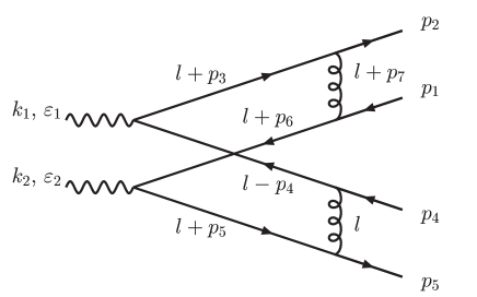
Figure 2: One of the diagrams contributing to the hard scattering amplitude of the process $\gamma\,\gamma\rightarrow\pi^{+}\,\pi^{-}$ at NLO.

$${\cal I}=\frac{(\mu^{2})^{-\varepsilon}}{2}\int\frac{d^{4+2\varepsilon}l}{(4\pi)^{4+2\varepsilon}}\frac{{\rm Tr}\left[\gamma_{\mu}\gamma_{5}\hskip 3.90451pt/P_{+}\gamma^{\mu}(\hskip 1.59029pt/l+\hskip 2.51563pt/p_{3})\hskip 2.33159pt/\varepsilon_{1}(\hskip 1.59029pt/l-\hskip 2.51563pt/p_{4})\gamma_{\nu}\gamma_{5}\hskip 3.90451pt/P_{-}\gamma^{\nu}(\hskip 1.59029pt/l+\hskip 2.51563pt/p_{5})\hskip 2.33159pt/\varepsilon_{2}(\hskip 1.59029pt/l+\hskip 2.51563pt/p_{6})\right]}{l^{2}(l+p_{3})^{2}(l-p_{4})^{2}(l+p_{5})^{2}(l+p_{6})^{2}(l+p_{7})^{2}},$$ (84)

with the momenta $p_{i}$ $(i=1,\ldots,7)$

$${}p_{1}=\overline{x}\,P_{+},\,\,\,\,p_{2}=x\,P_{+},\,\,\,\,p_{3}=k_{1}-\overline{y}\,P_{-},\,\,\,\,p_{4}=\overline{y}\,P_{-},$$

$${}p_{5}=y\,P_{-},\,\,\,\,p_{6}=y\,P_{-}-k_{2},\,\,\,\,p_{7}=\overline{x}\,P_{+}+y\,P_{-}-k_{2}.$$ (85)

The quantities $x$ and $\overline{x}\equiv 1-x$ ($y$ and $\overline{y}\equiv 1-y$) are the fractions of the momentum $P_{+}$ ($P_{-}$) shared between the quark and the antiquark in the $\pi^{+}$ ($\pi^{-}$).

With the aim of regularizing the IR divergences, the dimension of the integral is taken to be $D=4+2\varepsilon$.

The integral ${\cal I}$ is composed of one-loop 6-point tensor integrals of rank 0, 1, 2, 3 and 4. Performing the tensor decomposition and evaluating the trace, we obtain the integral ${\cal I}$ in the form

$${\cal I} = -2{\left(1+\varepsilon\right)}^{2}\,{\Big{[}}\,24\,s^{3}\,x\,\overline{x}\,y\,\overline{y}\,{\left(4\,\pi\,{\mu}^{2}\right)}^{4}\,I_{0}^{6}(12+2\,\varepsilon,\{1,1,1,1,1,5\})$$ (86)

$${}+6\,s^{3}\,\overline{y}\,y\,{\left(4\,\pi\,{\mu}^{2}\right)}^{4}\,I_{0}^{6}(12+2\,\varepsilon,\{1,4,1,1,2,1\})$$

$${}+2\,s^{3}\,\overline{y}\,\left(y-\overline{y}\right)\,{\left(4\,\pi\,{\mu}^{2}\right)}^{4}\,I_{0}^{6}(12+2\,\varepsilon,\{1,3,2,1,2,1\})$$

$${}+8\,s^{3}\,y\,\overline{y}\,{\left(4\,\pi\,{\mu}^{2}\right)}^{4}\,I_{0}^{6}(12+2\,\varepsilon,\{1,3,1,1,3,1\})$$

$${}+2\,s^{3}\,x\,y\,\overline{y}\,{\left(4\,\pi\,{\mu}^{2}\right)}^{4}\,I_{0}^{6}(12+2\,\varepsilon,\{1,2,2,2,1,2\})$$

$${}+s^{3}\,\overline{y}\,\left(y-\overline{y}\right)\,{\left(4\,\pi\,{\mu}^{2}\right)}^{3}\,I_{0}^{6}(10+2\,\varepsilon,\{1,2,2,1,2,1\})$$

$${}+s^{2}\,y\,\overline{y}\,\left(1+\varepsilon\right)\,\left(4\,\pi\,{\mu}^{2}\right)\,I_{0}^{6}(6+2\,\varepsilon,\{1,1,1,1,1,1\})$$

$${}+s\,\left(1+\varepsilon\right)\,\left(2+\varepsilon\right)\,{\left(4\,\pi\,{\mu}^{2}\right)}^{2}\,I_{0}^{6}(8+2\,\varepsilon,\{1,1,1,1,1,1\})$$

$${}+\ldots\mbox{75 similar terms}\,{\Big{]}}.$$

Next, performing the scalar reduction using the method described in the paper, we arrive at the following expression for the integral written in terms of the basic integrals:

$${\cal I}=8\,(1+\varepsilon)^{2}\left\{(4\,\pi\,{\mu}^{2})\left[\frac{\varepsilon}{\overline{x}}\,I_{4}^{1m}(6+2\,\varepsilon;-s/2,-s\,\overline{y}/2;-s\,y/2)\right.\right.$$ (87)

$${}+\frac{1+\varepsilon}{\overline{x}}\,I_{4}^{1m}(6+2\,\varepsilon;-s\,y/2,-s/2;-s\,\overline{y}/2)$$

$${}+\left(1+\varepsilon\left(1-\frac{x}{\overline{x}}\right)\right)\,I_{4}^{1m}(6+2\,\varepsilon;-s\,x/2,-s\,\overline{y}/2;-s\,(\overline{x}\,\overline{y}+x\,y)/2)$$

$${}\left.+\left(-\frac{x}{\overline{x}}+\varepsilon\left(1-\frac{x}{\overline{x}}\right)\right)\,I_{4}^{2me}(6+2\,\varepsilon;-s\,\overline{x}/2,-s\,\overline{y}/2;-s/2,-s\,(\overline{x}\,\overline{y}+x\,y)/2)\right]$$

$${}+\frac{1}{s}\left[\frac{1}{(\overline{x}-x)\,y}\left(\frac{2\,\overline{x}}{\varepsilon\,(\overline{x}-x)}+2-\frac{\overline{x}}{x}\right)\,I_{2}(4+2\,\varepsilon;-s\,\overline{x}/2)\right.$$

$${}+\frac{1}{(x-\overline{x})\,\overline{y}}\left(\frac{2\,x}{\varepsilon\,(x-\overline{x})}+2-\frac{x}{\overline{x}}\right)\,I_{2}(4+2\,\varepsilon;-s\,x/2)$$

$${}+\frac{1}{(\overline{y}-y)\,x}\left(\frac{2\,\overline{y}}{\varepsilon\,(\overline{y}-y)}+2-\frac{\overline{y}}{y}\right)\,I_{2}(4+2\,\varepsilon;-s\,\overline{y}/2)$$

$${}+\frac{1}{(y-\overline{y})\,\overline{x}}\left(\frac{2\,y}{\varepsilon\,(y-\overline{y})}+2-\frac{y}{\overline{y}}\right)\,I_{2}(4+2\,\varepsilon;-s\,y/2)$$

$${}+\left(\frac{(1-x\,\overline{y}-3\,y\,\overline{x})(1-y\,\overline{x}-3\,x\,\overline{y})}{x\,\overline{x}\,y\,\overline{y}\,(x-\overline{x})(y-\overline{y})}+\frac{2(\overline{x}\,\overline{y}+x\,y)(8\,x\,\overline{x}\,y\,\overline{y}-x\,\overline{x}-y\,\overline{y})}{\varepsilon\,x\,\overline{x}\,y\,\overline{y}\,(x-\overline{x})^{2}(y-\overline{y})^{2}}\right)$$

$${}\left.\left.\times\,I_{2}(4+2\,\varepsilon;-s\,(\overline{x}\,\overline{y}+x\,y)/2)+\frac{(\overline{x}\,\overline{y}+x\,y)}{x\,\overline{x}\,y\,\overline{y}}\,I_{2}(4+2\,\varepsilon;-s/2)\right]\right\}.$$

Here, $I_{2}$ is the two-point scalar integral in $D=4+2\,\varepsilon$ with $\nu_{i}=1$, while $I_{4}^{1m}$ and $I_{4}^{2me}$ are box scalar integrals in $D=6+2\,\varepsilon$. Analytic expressions for these integrals are given in the Appendix A. Expanding Eq. (87) up to order ${\cal O}(\varepsilon^{0})$, we finally get

$${\cal I}=\frac{i}{(4\,\pi)^{2}}\frac{8}{s}\left\{-\frac{1}{x\,\overline{y}}{\rm Li}_{2}(\overline{x}-x)-\frac{1}{y\,\overline{x}}{\rm Li}_{2}(x-\overline{x})-\frac{1}{y\,\overline{x}}{\rm Li}_{2}(\overline{y}-y)-\frac{1}{x\,\overline{y}}{\rm Li}_{2}(y-\overline{y})\right.$$ (88)

$${}+\frac{x\,\overline{y}+y\,\overline{x}}{x\,\overline{x}\,y\,\overline{y}}{\rm Li}_{2}\left(-(x-\overline{x})(y-\overline{y})\right)+\frac{\pi^{2}}{6}\frac{x\,\overline{y}+y\,\overline{x}}{x\,\overline{x}\,y\,\overline{y}}-\frac{\overline{x}\,\overline{y}+x\,y}{x\,\overline{x}\,y\,\overline{y}}\ln\!\left(\frac{s}{2\,\mu^{2}}\right)$$

$${}+\frac{(\overline{x}-2\,x)}{x\,y\,(\overline{x}-x)}\,\ln\left(\frac{s\,\overline{x}}{2\,\mu^{2}}\right)+\frac{(x-2\,\overline{x})}{\overline{x}\,\overline{y}\,(x-\overline{x})}\,\ln\left(\frac{s\,x}{2\,\mu^{2}}\right)$$

$${}+\frac{(\overline{y}-2\,y)}{x\,y\,(\overline{y}-y)}\,\ln\left(\frac{s\,\overline{y}}{2\,\mu^{2}}\right)+\frac{(y-2\,\overline{y})}{\overline{x}\,\overline{y}\,(y-\overline{y})}\,\ln\left(\frac{s\,y}{2\,\mu^{2}}\right)$$

$${}-\frac{x}{\overline{y}\,(x-\overline{x})^{2}}\,\ln^{2}\left(\frac{s\,x}{2\,\mu^{2}}\right)-\frac{\overline{x}}{y\,(x-\overline{x})^{2}}\,\ln^{2}\left(\frac{s\,\overline{x}}{2\,\mu^{2}}\right)$$

$${}-\frac{y}{\overline{x}\,(y-\overline{y})^{2}}\ln^{2}\!\left(\frac{s\,y}{2\,\mu^{2}}\right)-\frac{\overline{y}}{x\,(y-\overline{y})^{2}}\ln^{2}\!\left(\frac{s\,\overline{y}}{2\,\mu^{2}}\right)$$

$${}-\frac{(1-x\,\overline{y}-3\,y\,\overline{x})(1-y\,\overline{x}-3\,x\,\overline{y})}{x\,\overline{x}\,y\,\overline{y}\,(x-\overline{x})(y-\overline{y})}\,\ln\left(\frac{s\,(\overline{x}\,\overline{y}+x\,y)}{2\,\mu^{2}}\right)$$

$${}-\frac{(\overline{x}\,\overline{y}+x\,y)(8\,x\,\overline{x}\,y\,\overline{y}-x\,\overline{x}-y\,\overline{y})}{x\,\overline{x}\,y\,\overline{y}\,(x-\overline{x})^{2}(y-\overline{y})^{2}}\,\ln^{2}\left(\frac{s\,(\overline{x}\,\overline{y}+x\,y)}{2\,\mu^{2}}\right)$$

$$-\frac{2}{\hat{\varepsilon}}\left[\frac{x}{\overline{y}\,(x-\overline{x})^{2}}\,\ln\left(\frac{s\,x}{2\,\mu^{2}}\right)+\frac{\overline{x}}{y\,(x-\overline{x})^{2}}\,\ln\left(\frac{s\,\overline{x}}{2\,\mu^{2}}\right)\right.$$

$${}+\frac{y}{\overline{x}\,(y-\overline{y})^{2}}\,\ln\left(\frac{s\,y}{2\,\mu^{2}}\right)+\frac{\overline{y}}{x\,(y-\overline{y})^{2}}\,\ln\left(\frac{s\,\overline{y}}{2\,\mu^{2}}\right)$$

$${}\left.\left.+\frac{(\overline{x}\,\overline{y}+x\,y)(8\,x\,\overline{x}\,y\,\overline{y}-x\,\overline{x}-y\,\overline{y})}{x\,\overline{x}\,y\,\overline{y}\,(x-\overline{x})^{2}(y-\overline{y})^{2}}\,\ln\left(\frac{s\,(\overline{x}\,\overline{y}+x\,y)}{2\,\mu^{2}}\right)\right]\right\},$$

where $1/\hat{\varepsilon}=1/\varepsilon+\gamma-\ln(4\,\pi)$.

References

• [1] G. Passarino and M. Veltman, Nucl. Phys. B 160 (1979) 151; G. J. van Oldenborgh and J. A. M. Vermaseren, Z. Phys. C 46 (1990) 425; W. L. van Neerven and J. A. M. Vermaseren, Phys. Lett. B 137 (1984) 241.
• [2] A. I. Davydychev, Phys. Lett. B 263 (1991) 107.
• [3] Z. Bern, L. J. Dixon and D. A. Kosower, Phys. Lett. B 302 (1993) 299 [Erratum-ibid. B 318 (1993) 649] [arXiv:hep-ph/9212308].
• [4] Z. Bern, L. J. Dixon and D. A. Kosower, Nucl. Phys. B 412 (1994) 751 [arXiv:hep-ph/9306240].
• [5] O. V. Tarasov, Phys. Rev. D 54 (1996) 6479 [arXiv:hep-th/9606018].
• [6] J. Fleischer, F. Jegerlehner and O. V. Tarasov, Nucl. Phys. B 566 (2000) 423 [arXiv:hep-ph/9907327].
• [7] T. Binoth, J. P. Guillet and G. Heinrich, Nucl. Phys. B 572 (2000) 361 [arXiv:hep-ph/9911342]; G. Heinrich and T. Binoth, Nucl. Phys. Proc. Suppl.  89 (2000) 246 [arXiv:hep-ph/0005324].
• [8] T. Binoth, J. P. Guillet, G. Heinrich and C. Schubert, Nucl. Phys. B 615 (2001) 385 [arXiv:hep-ph/0106243].
• [9] J. M. Campbell, E. W. Glover and D. J. Miller, Nucl. Phys. B 498 (1997) 397 [arXiv:hep-ph/9612413].
• [10] A. Denner and S. Dittmaier, Nucl. Phys. B 658 (2003) 175 [arXiv:hep-ph/0212259].
• [11] G. Duplančić and B. Nižić, Eur. Phys. J. C 20 (2001) 357 [arXiv:hep-ph/0006249].
• [12] G. Duplančić and B. Nižić, Eur. Phys. J. C 24 (2002) 385 [arXiv:hep-ph/0201306].
• [13] A. I. Davydychev, J. Phys. A 25 (1992) 5587.
• [14] K. G. Chetyrkin and F. V. Tkachov, Nucl. Phys. B 192 (1981) 159; F. V. Tkachov, Phys. Lett. B 100 (1981) 65.
• [15] F. Jegerlehner and O. Tarasov, Nucl. Phys. Proc. Suppl. 116 (2003) 83 [arXiv:hep-ph/0212004].
• [16] A. T. Suzuki, E. S. Santos and A. G. Schmidt, Eur. Phys. J. C 26 (2002) 125 [arXiv:hep-th/0205158].
• [17] C. Anastasiou, E. W. Glover and C. Oleari, Nucl. Phys. B 565 (2000) 445 [arXiv:hep-ph/9907523]. A. T. Suzuki, E. S. Santos and A. G. Schmidt, arXiv:hep-ph/0210083.