Renormalization and factorization scale analysis of $\overline{b}b$ production in antiproton-proton collisions

Abstract:

There a sizable and systematic discrepancy between experimental data on the $\overline{b}b$ production in $\overline{\mathrm{p}}$p, $\gamma$p and $\gamma\gamma$ collisions and existing theoretical calculations within perturbative QCD. Before interpreting this discrepancy as a signal of new physics, it is important to understand quantitatively the ambiguities of conventional calculations. In this paper the uncertainty coming from renormalization and factorization scale dependence of finite order perturbation calculations of the total cross section of $\overline{b}b$ production in $\overline{\mathrm{p}}$p collisions is discussed in detail. It is shown that the mentioned discrepancy is reduced significantly if these scales are fixed via the Principle of Minimal Sensitivity.

1 Introduction

Heavy quark production in hard collisions of hadrons, leptons and photons has been considered as a clean test of perturbative QCD. It has therefore come as a surprise that the data on $\overline{b}b$ production in $\overline{\mathrm{p}}$p collisions at the Tevatron [1, 2], $\gamma$p collisions at HERA [3, 4] and $\gamma\gamma$ collisions at LEP2 [5, 6], some of them reproduced in Fig. 1, lie systematically by a factor of about 2-4 above the median of current theoretical calculations. For the first process the data are sufficiently copious to measure also the differential distribution in transverse momentum of the produced $b$ quark.

Figure 1: Data on $\overline{b}b$ production in $\overline{\mathrm{p}}$p [1], $\gamma$p [3, 4] and $\gamma\gamma$ [5, 6] collisions.

Although the data have sizable errors, this excess is too big to be accommodated within the current calculations. The comprehensive review of current status and related problems of the comparison of data on heavy quark production in all three collisions with QCD calculations can be found in [7, 8, 9].

The discrepancy between the D0 and CDF data on $\overline{b}b$ production and theoretical calculations [10], shown in Fig. 1a, has led to suggestions that it might represent the manifestation of effects of unintegrated gluon distribution function within the $k_{T}$-factorization approach [11, 12], or even a signal of supersymmetry [13, 14]. The agreement between the Tevatron data and the calculations [11, 14], reproduced in Fig. 2, is, indeed, quite impressive. On the other hand, before invoking new physics it is important to check that the data cannot be explained by more sophisticated application of QCD phenomenology.

Figure 2: D0 and CDF data on $\overline{b}b$ production compared to calculations using the $k_{T}$-factorization approach as implemented in CASCADE event generator [11] (left) and the supersymmetry [susy] (right).

The QCD calculations of heavy quark production in hard collisions of hadrons, leptons and photons depend on a number of inputs: $\alpha_{s}$, parton distribution functions (PDF) of colliding hadrons or photons, fragmentation functions of $b$ quarks, masses of heavy quarks, and the choice of renormalization (RS) and factorization (FS) scales $\mu$ and $M$. Quite recently, proper parameterization of fragmentation function has been argued [9] to be one of the possible sources of the disagreement of the CDF data [2] with NLO QCD calculations. There are also attempts to go beyond fixed order perturbative calculations by resumming the effects of large logs of the type $\ln(S/4m_{b}^{2})$ [15] or $\ln(p_{T}/m_{b})$ [16].

In this paper I investigate in detail the dependence of existing fixed order (LO and NLO) QCD calculations [17, 18] of the total cross section $\sigma_{tot}(\overline{b}b)$ in $\overline{\mathrm{p}}$p collisions on the choices of the renormalization and factorization scales. Similar analysis of $\overline{b}b$ production in $\gamma$p and $\gamma\gamma$ collisions will be presented elsewhere .

The paper is organized as follows. In the next Section basic facts relevant for further discussion are collected. In Section 3 some of the methods for selecting the renormalization and factorization scales are recalled and their relevance for the process under study discussed. This is followed in Section 4 by the discussion of the general form of the renormalization and factorization scale dependence of $\sigma_{tot}(\overline{b}b)$ at the NLO. Numerical results relevant for energies up to the Tevatron range are presented in Section 5 and conclusions drawn in Section 6.

2 Basic facts and formulae

The basic quantity of perturbative QCD calculations, the renormalized color coupling $\alpha_{s}(\mu)$, depends on the renormalization scale $\mu$ in a way governed by the equation

$$\frac{{\mathrm{d}}\alpha_{s}(\mu)}{{\mathrm{d}}\ln\mu^{2}}\equiv\beta(\alpha_{s}(\mu))=-\frac{\beta_{0}}{4\pi}\alpha_{s}^{2}(\mu)-\frac{\beta_{1}}{16\pi^{2}}\alpha_{s}^{3}(\mu)+\cdots,$$ (1)

where for $n_{f}$ massless quarks $\beta_{0}=11-2n_{f}/3$ and $\beta_{1}=102-38n_{f}/3$. The solutions of (1) depend beside $\mu$ also on the renormalization scheme (RS). At the NLO (i.e. taking into account first two terms in (1)) this RS can be specified, for instance, via the parameter $\Lambda_{\mathrm{RS}}$, corresponding to the renormalization scale for which $\alpha_{s}$ diverges . The coupling $\alpha_{(}\mu)$ is then given as the solution of the equation

$$\frac{\beta_{0}}{4\pi}\ln\left(\frac{\mu^{2}}{\Lambda^{2}_{\mathrm{RS}}}\right)=\frac{1}{\alpha_{s}(\mu)}+c\ln\frac{c\alpha_{s}(\mu)}{1+c\alpha_{s}(\mu)},$$ (2)

where $c=\beta_{1}/(4\pi\beta_{0})$. At the NLO the coupling $\alpha_{s}$ is thus a function of the ratio $\mu/\Lambda_{\mathrm{RS}}$ and the variation of the RS for fixed scale $\mu$ is therefore equivalent to the variation of $\mu$ for fixed RS. To vary both the renormalization scale and scheme is legitimate, but redundant. Let me emphasize that the choice of the RS is as important as the choice of renormalization scale. The fact that the coupling $\alpha_{s}(\mu)$, as well the coefficients of perturbation expansions, depend for fixed $\mu$ on the RS also implies that the existence of a “natural” physical scale in the problem, like the masses of heavy quarks in our case, is actually of no help in specifying unambiguously the NLO calculation. I will come back to this point in the next Section. If not stated otherwise, I will work in the conventional $\overline{\mathrm{MS}}$ RS and vary the renormalization scale $\mu$ only.

For hadrons the factorization scale dependence of PDF is determined by the system of evolution equations for quark singlet, nonsinglet and gluon distribution functions

$$\frac{{\mathrm{d}}\Sigma(M)}{{\mathrm{d}}\ln M^{2}} = P_{qq}(M)\otimes\Sigma(M)+P_{qG}(M)\otimes G(M),$$ (3)

$$\frac{{\mathrm{d}}G(M)}{{\mathrm{d}}\ln M^{2}} = P_{Gq}(M)\otimes\Sigma(M)+P_{GG}(M)\otimes G(M),$$ (4)

$$\frac{{\mathrm{d}}q_{\mathrm{NS}}(M)}{{\mathrm{d}}\ln M^{2}} = P_{\mathrm{NS}}(M)\otimes q_{\mathrm{NS}}(M),$$ (5)

where

$$\Sigma(x,M) \equiv \sum_{i=1}^{n_{f}}\left(q_{i}(x,M)+\overline{q}_{i}(x,M)\right),$$ (6)

$$q_{\mathrm{NS},i}(x,M) \equiv (q_{i}(x,M)+\overline{q}_{i}(x,M))-\frac{1}{n_{f}}\Sigma(x,M),~{}\forall i.$$ (7)

The splitting functions admit expansion in powers of $\alpha_{s}(M)$

$$P_{ij}(x,M)=\frac{\alpha_{s}(M)}{2\pi}P^{(0)}_{ij}(x)+\left(\frac{\alpha_{s}(M)}{2\pi}\right)^{2}P_{ij}^{(1)}(x)+\cdots,$$ (8)

where $P^{(0)}_{ij}(x)$ are unique, whereas all higher order splitting functions $P^{(j)}_{kl},j\geq 1$ depend on the choice of the factorization scheme (FS). Conversely, they can be taken as defining the FS, similarly as the higher order $\beta$-function coefficients $\beta_{i},i\geq 2$ in (1) define, together with $\Lambda_{\mathrm{RS}}$, the renormalization scheme. The equations (3-5) can be recast into evolution equations for $q_{i}(x,M),\overline{q}_{i}(x,M)$ and $G(x,M)$.

In all calculations of this exploratory study I took $n_{f}=4$ and solved the RG equation (2) numerically in order to guarantee correct behaviour of its solution for small renormalization scales.

3 Renormalization and factorization scales and their choice

Let us first recall the situation for processes involving the renormalization scale only. For them the QCD contribution to corresponding cross sections has the form ($a_{s}\equiv\alpha_{s}/\pi$)

$$r(Q)=a_{s}^{k}(\mu,{\mathrm{RS}})\left(r_{0}(Q)+r_{1}(Q/\mu,{\mathrm{RS}})a_{s}(\mu,{\mathrm{RS}})+r_{2}(Q/\mu,{\mathrm{RS}})a_{s}^{2}(\mu,{\mathrm{RS}})\cdots\right).$$ (9)

As an example, take the familiar ratio

$$R_{\tau}\equiv\frac{\Gamma(\tau^{-}\rightarrow\nu_{\tau}+{\mathrm{hadrons}})}{\Gamma(\tau^{-}\rightarrow\nu_{\tau}\mu^{-}\overline{\nu}_{\mu})}=3\left(1+r_{\tau}\right),$$ (10)

where the QCD correction $r_{\tau}$ is given by the expression (9) with $k=1$ and $r_{0}=1$. Theoretical consistency of the expansion (9) implies

$$r^{(N)}\equiv\sum_{j=k}^{N}r_{j-k}a_{s}^{j}~{}\Rightarrow~{}\frac{{\mathrm{d}}r^{(N)}}{{\mathrm{d}}\ln\mu}=O(a_{s}^{N+1}),$$ (11)

i.e. the derivative of the $N$-th order approximant $r^{(N)}$ with respect to $\ln\mu$ is of higher order than the appoximant $r^{(N)}$ itself. This requirement determines the dependence of the coefficients $r_{k}$ on $\mu$. For $r_{1}$ we get, for instance,

$$r_{1}(Q/\mu,{\mathrm{RS}})=kb\ln\frac{\mu}{Q}+r_{1}(1,{\mathrm{RS}})=kb\ln\frac{\mu}{\Lambda_{\mathrm{RS}}}-\rho(Q),$$ (12)

where $\rho(Q)\equiv kb\ln(Q/\Lambda_{\mathrm{RS}})-r_{1}(1,{\mathrm{RS}})$ is a renormalization scale and scheme invariant.

There are two general approaches to selecting the renormalization scale applicable in such circumstances: the Principle of Minimal Sensitivity [20] (PMS) and the method based on the concept of Effective Charges [21] (EC). In the first approach the emphasize is put on the stability of the results with respect to variations of $\mu$. In the absence of information on higher order perturbative terms in (9) the PMS approach is natural as it selects the point $\mu$ where the truncated perturbation expansion is most stable and has thus locally the property possessed by the all order result globally. The EC approach is based on the criterion of apparent convergence of perturbation expansions and the renormalization scale $\mu$ (and at higher orders other free parameters) is chosen in such a way that all higher order contributions vanish, i.e. demanding $r^{(N)}=r^{(k)}$ for all $N$. Whatever the choice of the renormalization scale $\mu$ scale we make, it is, however, certainly useful to investigate the stability of the results with respect to the variations of $\mu$.

In a fixed RS, both PMS and EC approaches can be phrased in geometrical terms as methods of selecting on a curve defined by the expression $r^{(N)}(\mu)$ some preferred point. The PMS approach selects the stationary point(s), whereas the EC method selects the point(s) given by the intersection of $r^{(N)}(\mu)$ with the curve corresponding to the lowest nontrivial order.

Figure 3: Renormalization scale dependence of the ratio $r_{\tau}$ in the $\overline{\mathrm{MS}}$ RS.

In Fig. 3 the $\mu$ dependence of the first three approximants $r^{(N)}_{\tau},N=1,2,3$ for the specific case of the quantity $r_{\tau}$ defined in (10) is plotted in $\overline{\mathrm{MS}}$ RS taking $\Lambda^{(3)}_{\overline{\mathrm{MS}}}=0.31$ GeV. Several features of this figure are worth noting.

• The conventional NLO approximation in the $\overline{\mathrm{MS}}$ RS, corresponding to the choice $\mu_{\overline{\mathrm{MS}}}=m_{\tau}=1.8$ GeV, gives substantially smaller result than that corresponding to the stationary point.

• Working in other RS, the same choice $\mu_{\mathrm{RS}}=m_{\tau}=1.8$ GeV would give a different result for $r_{\tau}(m_{\tau})$. In fact, any point on the NLO and NNLO curves can be obtained by setting $\mu_{\overline{\mathrm{MS}}}=m_{\tau}$ in appropriately chosen RS! The usual argument for using the $\overline{\mathrm{MS}}$ RS is that the associated $\alpha_{s}$ incorporates $\ln 4\pi-\gamma_{E}$, the artefact of dimensional regularization, and thus leads to smaller expansion coefficients $r_{k}$ than those of MS RS. But if the rate of convergence of perturbation expansions of physical quantities is the main criterion for the appropriate choice of the RS, than that based on the EC approach, rather than the $\overline{\mathrm{MS}}$ should be selected.

• The NLO and NNLO approximants $r^{(2)}_{\tau}$ and $r^{(3)}_{\tau}$ exhibit maxima, defining the PMS scales $\mu^{\mathrm{PMS}}_{\mathrm{\overline{\mathrm{MS}}}}$ and the corresponding PMS optimized results $r^{(N)}_{\mathrm{PMS}}(Q)$. No physical meaning should, however, be attached to numerical values of $\mu^{\mathrm{PMS}}_{\overline{\mathrm{MS}}}$ as in different RS the same maximum occurs at different scale .

• At both NLO and NNLO the PMS scales $\mu^{\mathrm{PMS}}_{\overline{\mathrm{MS}}}$ turn out to be quite close the scales $\mu^{\mathrm{EC}}_{\overline{\mathrm{MS}}}$ chosen by the EC approach. This fact holds, with some modification, for more complicated quantities as well.

• Although the preferred scales $\mu_{\overline{\mathrm{MS}}}^{\mathrm{PMS}}$ and $\mu_{\overline{\mathrm{MS}}}^{\mathrm{EC}}$ depend on the chosen RS, the PMS and EC optimized results $r^{(N)}_{\mathrm{PMS}}(Q)$ and $r^{(N)}_{\mathrm{EC}}(Q)$ do not! This fact follows directly from the geometrical meaning of the preferred points and is crucial for the uniqueness of the obtained predictions.

At higher orders and for more complicated physical quantities the situation is, however, not always so simple as sketched above. In some cases there is no genuine stationary point in the physical region and one must then look for some other measure of “most stable” region, or, on the contrary, there may be more stationary points to choose from. For physical quantities with two scales the general criterion of the EC approach does not lead to a unique point, but rather the curve $\mu(M)$ along which the higher order contributions vanish. However, even in these circumstances the PMS and EC approaches provide useful guidance to fixing the scales and thus defining the QCD predictions.

I now come to the central aspect of the choice of the renormalization and factorization scales. As emphasized by Politzer [22], there is no compelling reason for identifying these two scales. The point is that whereas the renormalization scale $\mu$ defines, roughly speaking, the lower limit on the virtualities of loop particles included in the definition of the renormalized coupling, the factorization scale $M$ specifies the upper limit on virtualities of partons included in the definition of dressed PDF. In other words, the renormalization scale reflects ambiguity in the treatment of short distances, whereas the factorization scale comes from similar ambiguity concerning large distances. It is therefore natural to keep the renormalization and factorization scales as independent free parameters of any finite order perturbative approximations. The calculations presented in the next two Sections demonstrate that at the NLO the cross section $\sigma_{tot}(\overline{b}b;M,\mu)$ depends, indeed, on these two scales in quite different way.

Identifying these two scales may actually lead to misleading conclusions concerning the stability of perturbative expressions. It may act in both ways, faking the “stability” where there is is fact none, but also hiding the genuine stability region when it lies away from the diagonal point $\mu=M$. At the NLO there is an additional degree of freedom (in fact an infinite number of them) related to the choice of the factorization scheme, specified by the higher order splitting functions $P_{ij}^{(1)}$. I will not exploit this freedom and throughout this paper stay within the conventional $\overline{\mathrm{MS}}$ FS.

4 General form of $\sigma_{tot}(Q\overline{Q})$

According to the factorization theorem the total cross section of heavy quark pair production in $\overline{\mathrm{p}}$p collisions at the center of mass energy $\sqrt{S}$ has the form

$$\sigma_{tot}(\overline{p}p\rightarrow\overline{Q}Q,S)=\int\!\!\!\!\int\!\!{\mathrm{d}x}{\mathrm{d}}y\sum_{ij}D_{i}^{\overline{p}}(x,M)D_{j}^{p}(y,M)\sigma_{ij}(s=xyS,M),$$ (13)

where partonic cross sections $\sigma_{ij}(s,M)\equiv\sigma(ij\rightarrow\overline{b}b,s,M)$, as well as PDF of the beam particles, $D_{j}^{\overline{p}}(M),D_{j}^{p}(M)$, depend on the factorization scale $M$. The theoretical calculations of heavy quark productions in refs. [7, 17, 18] are given in terms of the heavy quark pole mass, i.e. $m_{Q}$ appearing in the expressions for $\sigma_{ij}$ is just a fixed number.

The expression (13) is basically of nonperturbative nature. Fixed order perturbation theory enters if we insert into (13) the solutions of the evolution equations (3- 5) with the splitting functions $P_{ij}$ truncated to finite order (8) and calculate partonic cross sections $\sigma_{ij}(s,M)$ as power expansion in the coupling $\alpha_{s}(\mu)$

$$\sigma_{ij}(s,M)=\alpha_{s}^{2}(\mu)\sigma_{ij}^{(2)}(s)+\alpha_{s}^{3}(\mu)\sigma_{ij}^{(3)}(s,M,\mu)+\cdots,$$ (14)

taken at the renormalization scale $\mu$, which, as emphasized above, is in general unrelated to the factorization scale $M$. Summed to all orders of $\alpha_{s}$, the r.h.s of (14) is actually independent of $\mu$, whereas even the all-order sum of (14) depends on the factorization scale $M$. The latter dependence is cancelled by that of the PDF provided the splitting functions $P_{ij}$ in the evolution equations (3-5) are taken to all orders. This difference reflects the different roles played by the renormalization and factorization scales in expressions for physical quantities. If only finite order approximantions in (14) and (8) are used, as is in practice always the case, the partonic cross sections $\sigma_{ij}(s,M)$ become also $\mu$-dependent and the expression (13) thus becomes a function of both $\mu$ and $M$.

At the NLO, i.e. taking into account the first two terms in (14) and (8), we get (dropping for brevity the dependence on $S$ and specification of $\overline{b}b$ final state)

$$\sigma_{tot}^{\mathrm{NLO}}(M,\mu)=\alpha_{s}^{2}(\mu)\left\{\int\!\!\!\!\int{\mathrm{d}}x{\mathrm{d}}y\sum_{i=1}^{2n_{f}}q_{i}(x,M)q_{i}(y,M)\left[\sigma_{q\overline{q}}^{(2)}(xy)+\alpha_{s}(\mu)\sigma_{q\overline{q}}^{(3)}(xy,M,\mu)\right]+\right.$$

$$2\int\!\!\!\!\int\!{\mathrm{d}}x{\mathrm{d}}y\Sigma(x,M)G(y,M)\alpha_{s}(\mu)\sigma_{qG}^{(3)}(xy,M)+$$ (15)

$$\hskip 85.35826pt\left.\int\!\!\!\!\int\!{\mathrm{d}}x{\mathrm{d}}yG(x,M)G(y,M)\left[\sigma_{GG}^{(2)}(xy)+\alpha_{s}(\mu)\sigma_{GG}^{(3)}(xy,M,\mu)\right]\right\},$$

where the sum is understood to run over $n_{f}$ quarks and antiquarks, and the relation between PDF of protons and antiprotons was taken into account.

Theoretical consistency of (13) implies, similarly to (11), that the derivative of any finite order approximation thereof with respect to $\ln M^{2}$ is of higher order in $\alpha_{s}$ than such approximation itself. Performing this derivative for (15) we get

$$\frac{{\mathrm{d}}\sigma_{tot}^{\mathrm{NLO}}(M,\mu)}{{\mathrm{d}}\ln M^{2}} = \int\!\!\!\!\int\!{\mathrm{d}}x{\mathrm{d}}yG(x,M)G(y,M)W_{GG}(xy,M,\mu)\!+$$

$$\int\!\!\!\!\int\!{\mathrm{d}}x{\mathrm{d}}y\left[\sum_{i=1}^{2n_{f}}q_{i}(x,M)q_{i}(y,M)W_{qq}(xy,M,\mu)+\Sigma(x,M)G(y,M)W_{qG}(xy,M,\mu)\right].$$

Using (3-5) and denoting $\dot{f}\equiv\mathrm{d}f/\mathrm{d}\ln M^{2}$, the functions $W_{ij}$ are given as

$$\!\!W_{GG}(x,M,\mu) \!=\! \frac{\alpha_{s}^{3}(\mu)}{\pi}\left\{2\pi\dot{\sigma}_{GG}^{(3)}(x)+\!\!\int\!\!{\mathrm{d}}zP^{(0)}_{GG}(z)\sigma_{GG}^{(2)}(xz)\right\}+\cdots$$ (17)

$$W_{q\overline{q}}(x,M,\mu) \!=\! \frac{\alpha_{s}^{3}(\mu)}{\pi}\left\{2\pi\dot{\sigma}_{q\overline{q}}^{(3)}(x)+2\!\!\int\!\!{\mathrm{d}}zP^{(0)}_{qq}(z)\sigma_{q\overline{q}}^{(2)}(xz)\right\}+\cdots$$ (18)

$$W_{qG}(x,M,\mu) \!=\! \frac{\alpha_{s}^{3}(\mu)}{\pi}\left\{2\pi\dot{\sigma}_{qG}^{(3)}(x)+\!\!\int\!\!{\mathrm{d}}z\!\left[P^{(0)}_{qG}(z)\sigma_{q\overline{q}}^{(2)}(xz)+P^{(0)}_{Gq}(z)\sigma_{GG}^{(2)}(xz)\right]\!\right\}\!+\cdots$$ (19)

Theoretical consistency of (15) requires that the expressions standing in (17-19) by $\alpha_{s}^{3}$ vanish which, indeed, they do. For practical calculations it is suitable to rewrite the expression (13) as an integral

$$\sigma_{tot}(\overline{Q}Q,S)=\sum_{ij}\int{\mathrm{d}z}\Phi_{ij}(z,M)\sigma_{ij}(s=zS,M)$$ (20)

over the product of parton fluxes

$$\Phi_{ij}(z,M)\equiv\int\!\!\!\int{\mathrm{d}x}{\mathrm{d}}yD_{i}^{\overline{p}}(x,M)D_{j}^{p}(y,M)\delta(z-xy)$$ (21)

and partonic cross sections $\sigma_{ij}(z,M)$, both of which depend on the product of fractions $z\equiv xy$ only. Because the expressions for $\sigma_{ij}^{(3)}(s,M)$ as given in [17] correspond to $\mu=M$, I have restored their separate dependence on $\mu$ and $M$ by adding to $\sigma_{ij}^{(3)}(s,M)$ the term $2\beta_{0}\sigma_{ij}^{(2)}\ln(\mu^{2}/M^{2})$.

5 Results

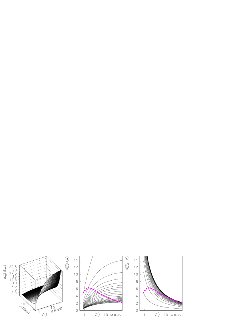
Figure 4: Graphical representation of $\sigma_{tot}^{\mathrm{LO}}(M,\mu)$ for $\sqrt{S}=630$ GeV: a) a two dimensional surface, together with its both projections, plotted for several values of $\mu$ in b) and $M$ in c).

In Fig. 4 the LO approximation $\sigma_{tot}^{\mathrm{LO}}(M,\mu)$ i.e. the sum of the terms proportional to $\alpha_{s}^{2}$ in (15), is plotted for $\sqrt{S}=630$ GeV as a two-dimensional surface $\sigma_{tot}^{\mathrm{LO}}(M,\mu)$, as well as a function of $M$ for fixed $\mu$, and as a function of $\mu$ for fixed $M$. There is no stability region of $\sigma_{tot}^{\mathrm{LO}}(M,\mu)$ in the sense of a stationary point on a two-dimensional surface. Keeping one of the scales fixed and varying the other (solid curves in Figs. 4b-c) leads in both cases to monotonous dependence on the latter. If, however, we set $\mu=M$, which means cutting the surface in Fig. 4a along the diagonal line, we obtain the dashed curve shown in both projections in the Figs. 4b-c, which has a spurious stationary point at about $\mu=M\doteq 1.5$ GeV, illustrating the point made at the end of Section 3.

Figure 5: Graphical representation of $\sigma_{tot}^{\mathrm{NLO}}(M,\mu)$ for $\sqrt{S}=62$ GeV.

The NLO approximant $\sigma_{tot}^{\mathrm{NLO}}(M,\mu)$ is represented graphically in Fig. 5 for $\sqrt{S}=62$ GeV, one of the energies investigated in [18], $m_{b}=5$ GeV and using GRV HO PDF. Setting $\mu=M$ we get the curves in Fig. 5a, where the individual contributions of gluon-gluon, quark-antiquark and quark-gluon channels are plotted as well. The quark-antiquark channel dominates for $M\gtrsim 2.5$ GeV, but the gluon-gluon one contributes significantly, too. At small $\mu=M$ the quark-quark contribution turns negative, as does eventually the gluon-gluon one, whereas that of the quark-gluon channel rises. The latter channel gives negative contribution at large values of $M$. To quantify the effects of the conventional assumption $\mu=M$, $\sigma_{tot}^{\mathrm{NLO}}(M,\mu=\kappa M)$ is plotted in Fig. 5b for three values of $\kappa=0.5,1,2$. The position of the stationary point as well as the corresponding value of $\sigma_{tot}^{\mathrm{NLO}}(M,\mu=\kappa M)$, depend on the value of $\kappa$, though not dramatically. Note that the positions of the maxima in Fig. 5b occur close to the intersections of the LO and NLO curves, defining the EC predictions. The spread between the three NLO curves at $M=m_{b}$ may be used as one of the measures of theoretical uncertainty of the conventional NLO calculations. The standard method of estimating this uncertainty is to set $M=\mu$ and vary this common scale within the interval $(m_{b}/2,2m_{b})$. Note, however, that the resulting band of values of $\sigma_{tot}^{\mathrm{NLO}}(\kappa m_{b},\kappa m_{b})$ depends on the choice of RS!

Keeping $\mu$ and $M$ as independent parameters and representing $\sigma_{tot}^{\mathrm{NLO}}(M,\mu)$ as two-dimensional surface in Fig. 5c or by the corresponding contour plot in Fig. 5d, reveals the saddle point located approximately at $\mu=2.4$ GeV, $M=3$ GeV. This saddle point, which defines the PMS result, lies close to the curve in Fig. 5d along which $\sigma^{\mathrm{NLO}}_{tot}(M,\mu)=\sigma^{\mathrm{LO}}_{tot}(M,\mu)$, defining the results preferred by the EC approach. Contrary to the PMS the Effective Charges approach does not lead to a unique prediction, but the whole range of values. At $\sqrt{S}=62$ GeV the saddle point lies also close to the point $\mu=M=m_{b}/2=2.5$ GeV, which is conventionally taken as the lower limit on the variation of the common scale $\mu=M=m_{b}$.

Figure 6: The same as in Fig. 5a,d but for $\sqrt{S}=630$ GeV.

As the collision energy increases, the situation changes in two respects:

• The relative contribution of the quark-antiquark channel decreases, its dominance at low energies being taken over by that of the gluon-gluon channel. The gluon-quark channel grows in importance at low values of $M$, roughly $M\lesssim 2$ GeV.

• The position of the saddle point moves in a highly “nondiagonal” manner away from the line $\mu=M$ and thus away from the conventional choice $\mu=M$. However, at all energies the saddle point stays close to the curve defining the EC results.

These changes are illustrated in Figs. 6, which shows the same plots as those in Fig. 5a,d but for $\sqrt{S}=630$ GeV. The energy dependence of the position of the saddle point $(\mu_{sad}(S),M_{sad}(S))$, represented by solid curves in Fig. 7a, illustrates yet again the different role of renormalization and factorization scales. Whereas $M_{sad}(S)$ stays constant up to about $\sqrt{S}\simeq 200$ GeV and then rises roughly as some power of $S$, $\mu_{sad}(S)$ first dips down to $\mu_{sad}\simeq 0.8$ GeV at about $\sqrt{S}\simeq 500$ GeV, before starting to rise at about the same rate as $M_{sad}(S)$ but remaining far below it. This large disparity between the values of renormalization and factorization scales at the saddle point provides the main reason for keeping these two scale as independent free parameters.

The “nondiagonal” position of the saddle point at higher energies leads to increasing difference between the PMS-optimized and conventional $\overline{\mathrm{MS}}$ results for $\sigma_{tot}^{\mathrm{NLO}}(S)$. This is illustrated in Fig. 7b which shows that the former rises more steeply in the region $100\lesssim\sqrt{s}\lesssim 500$ GeV than the standard calculations, after which they start to approach them again. To quantify this difference I plot in Fig. 7c the ratio:

$$R^{\mathrm{PMS}}(S)\equiv\frac{\sigma_{tot}^{\mathrm{NLO}}(M_{sad},\mu_{sad})}{\sigma_{tot}^{\mathrm{NLO}}(m_{b},m_{b},\overline{\mathrm{MS}})},$$ (22)

together with the ratia

$$R^{\kappa}(S)\equiv\frac{\sigma_{tot}^{\mathrm{NLO}}(\kappa m_{b},\kappa m_{b},\overline{\mathrm{MS}})}{\sigma_{tot}^{\mathrm{NLO}}(m_{b},m_{b},\overline{\mathrm{MS}})}$$ (23)

for $\kappa=0.5$ and $\kappa=2$. The PMS-optimized scales thus lead to predictions that are higher than those evaluated with the conventional choice $\mu=M=m_{b}$. For low energies the former are close to those corresponding to conventional calculations with $\kappa=0.5$, but at high energies $R^{\mathrm{PMS}}(S)$ rises steeply, reaching its maximum $R^{\mathrm{PMS}}(S)\doteq 2.2$ at about $\sqrt{S}=400$ GeV. At $\sqrt{S}=1800$ GeV $R^{\mathrm{PMS}}(S)\simeq 1.9$, which is about the same number as the factor characterizing the excess of D0 data over the conventional NLO QCD predictions in $\overline{\mathrm{MS}}$, which assume $\mu=M=m_{b}$. The fact that the difference between the results based on PMS-optimized and conventional choices of scales is a sensitive function of the collision energy provides a way for checking the phenomenological relevance of the optimization procedure based on the PMS idea of local stability.

Figure 7: a) Energy dependence of the position of the saddle point of $\sigma_{tot}^{\mathrm{NLO}}(b\overline{b})$ for $m_{b}=5$ GeV using GRV (solid curves) and MRS (dashed curves) PDF of the proton. The dotted curves show the same but for $m_{b}=11$ GeV. The dash-dotted curve shows the energy dependence of the average $p_{T}$ of the $b$-quark. b) The energy dependence of $\sigma_{tot}^{\mathrm{NLO}}(b\overline{b})$ in the conventional $\overline{\mathrm{MS}}$ RS (dotted curves) as well as the PMS-optimized prediction (solid curves), for two values of $m_{b}$. c) The ratia $R^{1/2}$, $R^{2}$ and $R^{\mathrm{PMS}}$ for $m_{b}=5$ GeV using the GRV (solid curves) and MRS (dashed curve) PDF. The dotted curves correspond to GRV PDF and $m_{b}=11$ GeV.

The results presented above have been obtained using fixed order perturbative QCD and could therefore be modified by the inclusion of the resummation of small-$x$ and/or large $p_{T}$ logs. Note that at the Tevatron the momentum fractions carried by partons producing the $b\overline{b}$ pair are typically larger than $0.006$, which is where the region of “small-$x$” usually starts. So one might expect the approach based on unintegrated PDF as used in CASCADE to improve the agreement with data, though it is not obvious by how much as CASCADE uses only a LO hard scattering cross sections. On the other hand, $R^{\mathrm{PMS}}$ peaks at $\sqrt{s}=400$ GeV, for which the mean parton fractions $\langle x\rangle\gtrsim 0.025$ are safely outside the small-$x$ region. Consequently, in the energy range where it is largest the difference between standard NLO calculations in $\overline{\mathrm{MS}}$ RS and PMS-optimized ones will likely survive the effects of small-$x$ resummation.

The LO calculation of the energy dependence of mean $p_{T}$ of the produced $b$-quarks, displayed by the dash-dotted curve in Fig. 7a, shows that it rises only very slowly and approaches $7$ GeV at the Tevatron range. This indicates that the resummation of large logs $\ln(p_{T}/m_{b})$ may be important for the tails of $p_{T}$ distributions, but cannot be expected to influence significantly the results for the total cross section.

The results discussed so far were obtained with the GRV HO parameterization of PDF of the proton. To check the dependence of the above conclusions on the choice of PDF, all the calculations were redone also with the MRS(R2) PDF used in [1]. As illustrated in Fig. 7a, there is noticeable difference in the location of saddle point at low energy, where the GRV saddle points are closer to the “diagonal” ones than the MRS(R2) ones, but as the energy increase both parameterizations give essentially the same results not only for the for the positions of the saddle points, but also for the energy dependence of the corresponding optimized total cross sections. This is illustrated in Fig. 7c, where the ratio $R^{\mathrm{PMS}}$ is plotted for both parameterizations. The conventional ratia $R^{1/2},R^{2}$ are so close for both parameterizations, that only those corresponding to GRV are displayed.

To get some feeling for the dependence of the above conclusions on the mass of the $b$-quark, Figure 7 shows also the results obtained for $m_{b}=11$ GeV, which is roughly the transverse mass $m_{T}=\sqrt{m_{b}^{2}+p_{T}^{2}}$ at the Tevatron. Clearly, the difference between standard and PMS-optimized calculations decreases with increasing $m_{b}$ and the region of largest $R^{\mathrm{PMS}}$ shifts, as expected, to larger energies.

6 Summary and conclusions

The results of this exploratory study demonstrate the sensitivity of the NLO QCD calculations of the total cross section $\sigma_{tot}^{\mathrm{NLO}}(\overline{b}b)$ to the choice of the renormalization and factorization scales. In particular they show that the conventional assumption of identifying these two scales leads at high energies far away from the region of local stability as quantified by the Principle of Minimal Sensitivity criterion. As a result, the conventional NLO calculations yield results that are lower than the PMS-optimized ones, at the Tevatron energies by a factor of about 2, which is approximately the factor needed to bring the conventional calculations into agreement with the D0 and CDF data.

This observation cannot, however, be directly used as an explanation of the excess of the Tevatron data over conventional NLO predictions because it concerns the total cross section rather than the differential distribution $\mathrm{d}\sigma/{\mathrm{d}}p_{T}$ measured by the D0 and CDF Collaborations. The ongoing analysis [23] of renormalization and factorization scale dependence of such differential distribution indicates that the situation for such distribution is similar to that discussed in this paper, with additional dependence of the stability region on $p_{T}$ of the $b$-quark. This paper will also address the question of the stability of the NLO QCD calculations of the top quark production at both Tevatron and LHC.

I also don’t claim that the choice of the renormalization and factorization scale via the PMS-optimization explains fully the observed discrepancy between data and conventional NLO QCD calculation of $\sigma_{tot}^{\mathrm{NLO}}(\overline{b}b)$ or that it is the only effect that might be responsible for such discrepancy. The purpose of this paper is rather to point out yet another source of theoretical uncertainty of higher order QCD calculations of quantities like $\sigma_{tot}^{\mathrm{NLO}}(\overline{b}b)$ that should be properly taken into account before drawing conclusions from the comparisons with experimental data.

- [1] B. Abbott et al. (D0 Collab.): Phys. Rev. Lett. 85 (2000), 5068, (hep-ex/0008021)
- [2] D. Acosta et al. (CDF Collab.): Phys. Rev. D65 (2002), 052005, (hep-ex/0111359)
- [3] C. Adloff et al (H1 Collab.): Phys. Lett. B467 (1999), 156 and Erratum: Phys. Lett. B518 (2001), 331
- [4] J. Breitweg et al. (ZEUS Collab.): Eur. Phys. J. C18 (2001), 625, (hep-ex/0011081)
- [5] M. Acciarri et al. (L3 Collab.): Phys. Lett. B503 (2001), 10
- [6] OPAL Collab.: OPAL Physics Note PN455, August 2000
- [7] S. Frixione: Proceedings of International Europhysics Conference on HEP, Budapest, July 2001, hep-ph/0111368
- [8] P. Nason: Proceedings of Interbational Symposium on Lepton and Photon Interactions at High Energy, Rome, July 2001, hep-ph/0111024
- [9] M. Cacciari and P. Nason: Phys. Rev. Lett. 89 (2002), 122003-1
- [10] S. Frixione and M. Mangano: Nucl. Phys. B483 (1997), 321, (hep-ph/9605270)
- [11] H. Jung: Phys. Rev. D65 (2002), 034015
- [12] A. V. Lipatov, V. A. Saleev and N. P. Zotov: hep-ph/0112114
- [13] E. Berger et al: Phys. Rev. Lett. 86 (2001), 4231, (hep-ph/0012001)
- [14] E. Berger: hep-ph/0201229
- [15] S. Catani, M. Ciafaloni and F. Hautman: Nucl. Phys. B366 (1991), 135
- [16] M. Cacciari, M. Greco and P. Nason: JHEP 05 (1998), 007, (hep-ph/9803400)
- [17] P. Nason, S. Dawson and R. K. Ellis: Nucl. Phys. B303 (1988), 607
- [18] G. Altarelli, M. Diemoz, G. Martinelli and P. Nason: Nucl. Phys. B308 (1988), 724
- [19] J. Chýla, hep-ph/0111469.
- [20] P. M. Stevenson, Phys. Rev. D21 (1981), 2916
- [21] G. Grunberg, Phys. Rev. D29 (1984), 2315
- [22] H. D. Politzer, Nucl. Phys. B192 (1984), 493
- [23] J. Srbek: in preparation