Do the KamLAND and Solar Neutrino Data Rule out Solar Density Fluctuations?

Abstract

We elucidate effects of solar density fluctuations on neutrino propagation through the Sun. Using data from the recent solar neutrino and KamLAND experiments we provide stringent limits on solar density fluctuations. It is shown that the neutrino data constrains solar density fluctuations to be less than $\beta=0.05$ at the 70 % confidence level, where $\beta$ is the fractional fluctuation around the value given by the Standard Solar Model. We find that the best fit to the combined solar neutrino and KamLAND data is given by $\beta=0$.

I Introduction

The evolution of the Sun is modeled using a standard set of input parameters describing the physics of the interior, including thermodynamic properties (equation of state), energy transfer through solar matter (opacity) and the rates of the nuclear reactions that power the Sun (astrophysical S-factors). The resulting detailed models of the Sun predict temperature, density, composition profiles, and neutrino fluxes coming from the nuclear fusion reactions. Recently the Standard Solar Model (SSM) has been enjoying a tremendous success. Its predictions (see Bahcall:2000nu ; Brun:1998qk ) have withstood the observational and experimental tests very well. For example, SSM predicts frequencies of the pressure (p-mode) vibrations which can be observed on the solar surface. Observation and analysis of these oscillations, called helioseismology, provide detailed information about the Solar interior (for a thorough introduction to helioseismology and review of the observational data see Ref. Christensen-Dalsgaard:2002ur ). The helioseismological information can be inverted to obtain the sound-speed profile throughout the Sun. The speed of sound in the Sun is determined by combining the density and temperature profiles which are predicted using the Standard Solar Model. The sound speeds of solar models that include element diffusion agree with helioseismological measurements to better than 0.2 % Bahcall:1996qw ; Bahcall:1998wm . Another test of SSM was achieved by the neutral-current measurements at the Sudbury Neutrino Observatory (SNO) Ahmad:2002jz . These measurements yield a total (all flavors) ⁸B solar neutrino flux which is in very good agreement with the Standard Solar Model predictions. Identifying the precise nuclear reactions that power the Sun would be another valuable constraint on the SSM Adelberger:1998qm . It is generally believed that the nuclear fusion reactions that power the Sun take place in the so-called pp cycle. The recent data also provides a stringent limit (less than 7 %) to the amount of energy that the Sun produces via the CNO fusion cycle Bahcall:2002jt .

Given these recent successes of the Standard Solar Model and the quality of the experimental data currently being taken, perhaps the time has come to test some of the other aspects of the model. One such test, namely looking for fingerprints of the solar density fluctuations in solar neutrino spectra was already considered extensively starting in the early 1990’s Loreti:1994ry ; Balantekin:1996pp ; Nunokawa:1996qu ; Burgess:1996mz ; Nunokawa:1997dp ; Bamert:1997jj ; Torrente-Lujan:1998pf ; Bykov:2000ze , but at that time the solar neutrino data were not accurate enough to make a definitive statement. Such fluctuations may provide an additional probe of the physics of the deep solar interior Burgess:2002we . For example, evolution theories of stars, in addition to p-modes, also predict the existence of buoyancy-driven gravity modes (g-modes). Whether g-modes are actually excited in the Sun is an open question. These modes are exponentially damped in the convective zone of the Sun; unlike the p-modes it is not possible to observe the resulting very small amplitudes of the g-modes on the surface of the Sun using current techniques even if they are indeed excited in the Sun. It is argued that g-modes in the Sun can be excited by turbulent stresses in the convective zone Kumar:1995gq or by magnetic fields in the radiative zone Burgess:2002we . Although the latter hypothesis requires large magnetic fields in the Sun, a magnetic field as large as $10^{7}$ G in the radiative zone seems to be permitted by the helioseismic data Couvidat:2002bs . It should be emphasized that temperature fluctuations associated with the large-amplitude g-mode oscillations would have significantly reduced the neutrino flux produced in the core of the Sun. Observational upper limits on the surface velocity amplitudes (as well the direct measurement of the total solar neutrino flux at SNO) rule out such large-amplitude g-mode oscillations Bahcall:zk . The scenario we discuss here is the possibility of smaller-amplitude g-mode oscillations or some other mechanism causing fluctuations in the density profile of the Sun affecting neutrinos only through their interaction with the matter. (For an alternative mechanism for producing density fluctuations in the Sun through magneto-hydrodynamic waves see Ref. Dzhalilov:1998np ). At the very least it is important to investigate what limits the solar neutrino data (supplemented by the constraints of the KamLAND reactor neutrino measurements) would place on the size of such fluctuations.

Our goal in this paper is to revisit the subject of density fluctuations and investigate limits placed by the recent solar and reactor neutrino experiments on the amount of fluctuation. Our preliminary attempts to use earlier SNO data were presented in Ref. Balantekin:2001dx . In the next section we review the formalism and summarize our method for doing the global analysis. In Section 3 we present our results and discuss their implications.

II Solar Density Fluctuations

We will assume that the electron density $N_{e}$ fluctuates around the value, $\langle N_{e}\rangle$, predicted by the SSM

$$N_{e}(r)=(1+\beta F(r))\langle N_{e}(r)\rangle,$$ (1)

and that the fluctuation $F(r)$ obeys

$$\langle F(r)\rangle = 0$$

$$\langle F(r_{1})F(r_{2})\rangle = f_{12}$$

$$\langle F(r_{1})F(r_{2})F(r_{3})\rangle = 0$$

$$\langle F(r_{1})F(r_{2})F(r_{3})F(r_{4})\rangle = (f_{12}f_{34}+f_{13}f_{24}+f_{14}f_{23})$$ (2)

$$\vdots$$

where $f_{ij}=f(|r_{j}-r_{i}|)$ gives the correlation between fluctuations in different places. In Eq. (1) we can interpret the quantity $\beta$ as the fraction of the fluctuation around the density given by the SSM. Throughout the current paper, we consider the case of delta-correlated (white) noise:

$$f(r)=2\tau\delta(r),$$ (3)

with the correlation length $\tau$ as a parameter. We discuss the limitations of this assumption later in this section. The Hamiltonian describing neutrino evolution in matter can be written as as sum of two terms:

$$H=H_{0}+B(r)M,$$ (4)

where $H_{0}$ is the standard Mikheev-Smirnov-Wolfenstein (MSW) Hamiltonian Wolfenstein:1977ue (for a brief review see Balantekin:1998yb ) with the average electron density $\langle N_{e}\rangle$, $B(r)$ is the fluctuating c-number and $M$ is a constant operator. For the two-flavor mixing $H_{0}$ governs the time-evolution in the SSM density:

$$i\frac{\partial}{\partial t}\left(\begin{array}[]{c}\nu_{e}\\ \nu_{x}\end{array}\right) = \frac{\delta m^{2}}{4E}\left(\begin{array}[]{cc}\zeta(t)-\cos 2\theta&\sin 2\theta\\ \sin 2\theta&-(\zeta(t)-\cos 2\theta)\end{array}\right)$$ (12)

$$\times\left(\begin{array}[]{c}\nu_{e}\\ \nu_{x}\end{array}\right)$$

where

$$\zeta(r)=\frac{2\sqrt{2}G_{F}E}{\delta m^{2}}\langle N_{e}(r)\rangle,$$ (13)

$\theta$ is the vacuum neutrino mixing angle, $\delta m^{2}$ is the difference in the squared masses of the two neutrino species, $E$ is the neutrino energy, and $\langle N_{e}\rangle$ is the averaged electron number density given by the SSM. In Eq. (12), $\nu_{x}$ is an arbitrary combination of $\nu_{\mu}$ and $\nu_{\tau}$ Balantekin:1999dx . The fluctuating term $B(t)$ is given by

$$B(r)=\beta F(r)\frac{G_{F}}{\sqrt{2}}\langle N_{e}(r)\rangle,$$ (14)

and $M=\sigma_{3}$. Using Eq. (2) one can show that the fluctuation of $B(r)$ satisfies the conditions

$$\langle B(r_{1})\rangle = 0$$

$$\langle B(r_{1})B(r_{2})\rangle = \alpha^{2}f_{12}$$

$$\langle B(r_{1})B(r_{2})B(r_{3})\rangle = 0$$

$$\langle B(r_{1})B(r_{2})B(r_{3})B(r_{4})\rangle = \alpha^{4}(f_{12}f_{34}+f_{13}f_{24}+f_{14}f_{23})$$ (15)

$$\vdots$$

where

$$\alpha(r)=-\frac{G_{F}}{\sqrt{2}}\beta\langle N_{e}\rangle,$$ (16)

It was shown in Refs. Loreti:1994ry ; Balantekin:1996pp that with the white noise assumption of Eq. (3) the fluctuation-averaged neutrino density matrix satisfies the equation

$$\frac{\partial}{\partial t}\langle\rho(t)\rangle=-\alpha^{2}\tau[M,[M,\langle\rho(t)\rangle]]-i[H_{0}(t),\langle\rho(t)\rangle].$$ (17)

For the two-flavor case, depicted in Eqs. (12) and (14), after calculating the commutators Eq. (17) can be re-written as a $3\times 3$ matrix equation Loreti:1994ry ; Balantekin:1996pp

$$\frac{\partial}{\partial t}\left(\begin{array}[]{c}z\\ x\\ y\end{array}\right)=-2\left(\begin{array}[]{ccc}0&0&D\\ 0&k&-A(t)\\ -D&A(t)&k\end{array}\right)\left(\begin{array}[]{c}z\\ x\\ y\end{array}\right),$$ (18)

where the individual elements of the density matrix are

$$z = 2\langle\nu_{e}^{*}\nu_{e}^{\phantom{*}}\rangle-1$$

$$x = 2\>\hbox{Re}\,\langle\nu_{\mu}^{*}\nu_{e}^{\phantom{*}}\rangle$$

$$y = 2\>\hbox{Im}\,\langle\nu_{\mu}^{*}\nu_{e}^{\phantom{*}}\rangle.$$ (19)

In these equations $\nu_{f}$ is the probability amplitude for the neutrino flavor $f$, and we introduced the definitions

$$A(t)\equiv\frac{\delta m^{2}}{4E}(\zeta(t)-\cos 2\theta),\quad D\equiv\frac{\delta m^{2}}{4E}\sin 2\theta,$$ (20)

and

$$k=G_{F}^{2}\langle N_{e}(r)\rangle^{2}\beta^{2}\tau.$$ (21)

We numerically solved Eq. (18) using the technique developed in Ref. Ohlsson:1999um which we summarize. We first consider the constant density case. If we represent the column vector in Eq. (18) by ${\cal R}(t)$ and the matrix governing its time-evolution by ${\cal K}$ ($d{\cal R}/dt={\cal K}{\cal R}$), for constant density one can write

$${\cal R}(t)=\exp{[{\cal K}t]}{\cal R}(t=0)=U(t){\cal R}(t=0).$$ (22)

The exponential in Eq. (22) can be calculated using Cayley-Hamilton theorem which states that for any matrix $M$, the eigenvalue in the characteristic equation can be replaced with the matrix itself. For a $3\times 3$ matrix we get:

$$e^{M}=a_{0}I+a_{1}M+a_{2}M^{2}.$$ (23)

The coefficients can be found by by substituting eigenvalues $\lambda_{i}$ of $M$ into

$$e^{\lambda_{i}}=a_{0}+\lambda_{i}a_{1}+\lambda_{i}^{2}a_{2}.$$ (24)

In a medium with varying density (where the variables $A$ and $k$ are changing), time evolution can be calculated by dividing neutrino path into small intervals in which potential can be approximated as a constant. Then the total evolution operator is product of evolution operators for all intervals:

$$U=U_{N}U_{N-1}.......U_{2}U_{1}.$$ (25)

Care must be taken to ensure that the intervals chosen are smaller than the oscillation length.

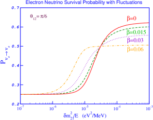
Figure 1: Mean survival probabilities for the SSM density profile and $\sin\theta_{12}=\pi/6$ calculated as described in the text. The correlation length is chosen to be 10 km and the probabilities are plotted for the percentage fluctuation values of $\beta=0$ (solid line), $\beta=0.015$ (dashed line),$\beta=0.03$ (dotted line),$\beta=0.06$ (dot-dashed line).

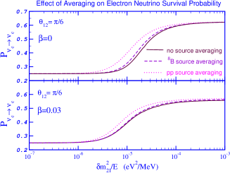
Figure 2: The effect of source averaging on various components of the mean survival probability without ($\beta=0$) and with ($\beta=0.3$) fluctuations. The SSM density profile of Ref. Bahcall:2000nu , the mixing angle of $\sin\theta_{12}=\pi/6$, and the correlation length of 10 km are used. The solid lines are the survival probabilities without source averaging. The dashed lines represent the source-averaged survival probabilities of ⁸B neutrinos and the dotted-line those of the pp neutrinos.

To give a feeling about the solutions of Eq. (18) we show in Figure 1 mean survival probabilities obtained by solving it numerically as described above for different values of $\beta$ and a correlation length of $\tau=10$ km. From this figure one observes that the effect of the fluctuations is more dominant when the neutrino parameters and the average density are such that neutrino evolution in the absence of fluctuations is adiabatic. For the two-flavor case one can write the electron neutrino survival probability as Haxton:dm ; Balantekin:1998yb

$$P(\nu_{e}\rightarrow\nu_{e})=\frac{1}{2}+\frac{1}{2}\cos 2\theta\cos 2\theta_{M}(1-2|\psi_{2}|^{2}),$$ (26)

where $|\psi_{2}|^{2}$ is the probability of observing the second matter eigenstate on the surface of the Sun (calculated with the initial condition that the neutrinos start in the first matter eigenstate), also known as the hopping probability, and the matter angle is given as

$$\cos 2\theta_{M}=-A/\sqrt{A^{2}+D^{2}}.$$ (27)

In Eq. (26) $\cos 2\theta_{M}$ is the matter angle where the neutrinos are created. Note that the $\cos 2\theta_{M}$ is zero at the MSW resonance. If the neutrino propagation is adiabatic when $\beta$ is set to zero, the hopping probability is zero. However when the fluctuations are turned on they cause some hopping, yielding a small but non-zero $|\psi_{2}|^{2}$, which grows with $\beta$. Consequently when $\beta\neq 0$, the absolute value of the second term on the right-hand side of Eq. (26) is always less than its value when $\beta=0$. If the value of $\delta m^{2}/E$ is such that neutrinos are produced at the MSW resonance density then the cosine of the initial matter angle is zero, and Eq. (26) predicts a survival probability of $1/2$ no matter what the value of $\beta$ is. For smaller values of $\delta m^{2}/E$ the initial value of the matter angle is negative, yielding a higher survival probability as compared to the $\beta=0$ case. For larger values of $\delta m^{2}/E$ the initial value of the matter angle is positive, yielding a lower survival probability as compared to the $\beta=0$ case. This behavior is clearly evident in Figure 1.

There are two constraints on the value of the correlation length. In averaging over the fluctuations we assumed that the correlation function is a delta function (cf. Eq. (3)). In the Sun it is more physical to imagine that the correlation function is like a step function of size $\tau$. Assuming that the logarithmic derivative is small, which is accurate for the Sun, delta-correlations are approximately the same as step-function correlations if the condition

$$\tau\ll\left(\sin 2\theta\frac{\delta m^{2}}{2E}\right)^{-1}$$ (28)

is satisfied Balantekin:1996pp . Eq. (28) can be rewritten as

$$\tau({\rm km})\ll 3.95\times 10^{-4}\frac{E({\rm MeV})}{\sin 2\theta\>\delta m^{2}({\rm eV}^{2})}.$$ (29)

A second constraint on the correlation length is provided by the helioseismology. Density fluctuations over scales of $\sim 1000$ km seem to be ruled out Christensen-Dalsgaard:2002ur ; Burgess:2002we ; Castellani:1997pk . On the other hand current helioseismic observations are rather insensitive to density variations on scales close to $\sim 100$ km Burgess:2002we .

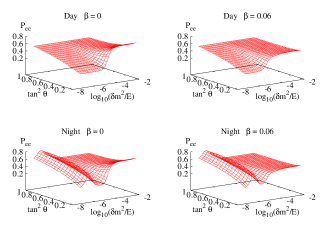
Figure 3: Source-averaged survival probabilities for ⁸B neutrinos with and without solar-density fluctuations detected at the location of SNO during the day and the night. The SSM density profile of Ref. Bahcall:2000nu and the correlation length of 10 km are used.

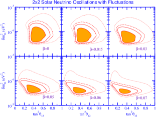
Figure 4: Allowed regions of the neutrino parameter space with solar-density fluctuations when only solar neutrino experiments (chlorine, all three gallium, SNO and SK experiments) are included in the analysis. The SSM density profile of Ref. Bahcall:2000nu and the correlation length of 10 km are used. The case with no fluctuations ($\beta=0$) are compared with results obtained with the indicated fractional fluctuation. The shaded area is the 70 % confidence level region. 90 % (solid line), 95 % (dashed line), and 99 % (dotted line) confidence levels are also shown.

III Results and Discussion

In our analysis we used a covariance approach the details of which are described in Ref. Balantekin:2003dc . We use 93 data points in our analysis; the total rate of the chlorine experiment (Homestake Cleveland:nv ), the average rate of the gallium experiments (SAGE Abdurashitov:2002nt , GALLEX Hampel:1998xg , GNO Altmann:2000ft ), 44 data points from the SK zenith-angle-spectrum Fukuda:2001nj , 34 data points from the SNO day-night-spectrum Ahmad:2001an and 13 data points from the KamLAND spectrum Eguchi:2002dm . We took into account the distribution of the neutrino sources in the Sun. Specifically we divided the Sun into several shells, calculated the survival probability numerically for neutrino paths and averaged the survival probabilities over the initial source distributions. Similarly we considered the effects of the matter density of the Earth (the day-night effect) by solving neutrino evolution equations numerically. We illustrate the effects of source averaging (with and without fluctuations) in Figures 2 and 3. In Figure 2 we show the source-averaged survival probability separately for the pp and ⁸B neutrinos. In this figure the solid line represents the survival probability of the neutrinos coming from a single point (the center of the Sun) contrasted to the source-averaged cases. For $\beta=0$, for a given $\delta m^{2}$, neutrino energy, and mixing angle neutrino evolution is adiabatic for the region of interest shown in the graph. In contrast, for $\beta\neq 0$, one has a non-zero, but small hopping probability. When the neutrinos are created over a finite-size region (instead of a single point) source-averaged survival probabilities do not coincide at large $\delta m^{2}/E$ values with the point-source survival probability unlike the $\beta=0$ case. Fluctuations also reduce the effect of the averaging. In Figure 3 we present the source-averaged survival probabilities detected at the location of SNO for ⁸B neutrinos with and without solar-density fluctuations. To calculate this figure we used the day and night live-time information from Ref. HOWTOSNO . One again observes that fluctuations smoothen the survival probabilities.

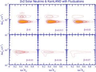
Figure 5: Allowed regions of the neutrino parameter space with solar-density fluctuations when the data from the solar neutrino experiments (chlorine, all three gallium, SNO and SK experiments) and the KamLAND data are included in the analysis. The SSM density profile of Ref. Bahcall:2000nu and the correlation length of 10 km are used. The case with no fluctuations ($\beta=0$) are compared with results obtained with the indicated fractional fluctuation. The shaded area is the 70 % confidence level region. 90 % (solid line), 95 % (dashed line), and 99 % (dotted line) confidence levels are also shown.

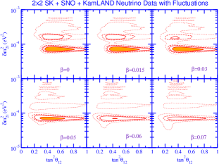
Figure 6: Allowed regions of the neutrino parameter space with solar-density fluctuations when the data from the solar neutrino experiments detecting only the high energy ⁸B neutrinos (SNO and SK experiments) and the KamLAND data are included in the analysis. The SSM density profile of Ref. Bahcall:2000nu and the correlation length of 10 km are used. The case with no fluctuations ($\beta=0$) are compared with results obtained with the indicated fractional fluctuation. The shaded area is the 70 % confidence level region. 90 % (solid line), 95 % (dashed line), and 99 % (dotted line) confidence levels are also shown.

We next turn our attention to parameter-space searches. In Ref. Balantekin:2003dc from a global analysis of solar neutrino and KamLAND data we found for electron neutrino oscillations into another active flavor, the best fit values of $\tan^{2}\theta_{12}\sim 0.46$ for the mixing angle between first and second generations, $\tan^{2}\theta_{13}\sim 0$ for the mixing between first and third generations, and $\delta m_{21}^{2}\sim 7.1\times 10^{-5}$ eV². Other groups doing similar analyses found very similar best fit values allothers . In Ref. Balantekin:2003dc $\beta$ was taken to be zero. We find that non-zero values of $\beta$ reduces the size of the allowed region as shown in Figure 4. In this figure allowed regions of the neutrino parameter space are shown for different values of $\beta$ when all the solar neutrino experiments (chlorine, all three gallium, SNO and SK experiments) are included in the analysis. Although the minimum value of $\chi^{2}$ is achieved when $\beta=0$, one observes that for values of $\beta$ as large as 0.07 allowed regions remain even at the 70 % confidence level. Thus we conclude that solar neutrino data alone does not significantly constrain the fluctuation parameter. Note that for larger values of $\beta$ the region with larger values of $\delta m^{2}$ are no longer allowed. Since KamLAND data favor larger values of $\delta m^{2}$, incorporating KamLAND results dramatically reduces the allowed region in parameter space as shown in Figure 5. Again the he minimum value of $\chi^{2}$ is achieved when $\beta=0$. However, in contrast to the calculation presented in Figure 4, one can put stringent limits on the amount of fluctuation. We find that $\beta<0.05$ at the 70 % confidence level, $\beta<0.06$ at the at the 90 % confidence level, and $\beta<0.07$ at the at the 95 % confidence level.

Let us recall that both calculations are done for a value of $\tau=10$ km for the correlation length. Note that only the combination $\beta^{2}\tau$ enters into the calculation (cf. Eq. (21). Hence the $\beta$ values can be scaled by adjusting the value of $\tau$ and for larger correlation lengths the limits quoted above get tighter. However one cannot consider arbitrarily large values of the correlation length. Our formulation of the problem (the delta-function correlation approximation) becomes unrealistic for larger values of $\tau$ as we illustrated in Eq. (29). In we insert the best fit (minimum $\chi^{2}$) values of $\delta m^{2}\sim 7.1\times 10^{-5}$ eV² and $\tan^{2}\theta\sim 0.46$ into Eq. (29) we find

$$\tau({\rm km})<6E({\rm MeV}).$$ (30)

Hence for lower-energy (pp) neutrinos the reliable correlation lengths are smaller then 10 km. However for higher energy (⁸B) neutrinos one can safely consider longer correlation lengths. For both SK and SNO the energy threshold is $\sim 5$ MeV for which Eq. (30) yields $\tau<30$ km. To explore this feature we repeat our analysis considering only SK and SNO data together with the KamLAND data. We show the allowed regions of the parameter space in Figure 6. In this figure for better comparison to Figure 5 we took $\tau$ to be 10 km, however even $\tau=20$ km would be reasonable. The best fit is still with $\beta=0$. We find that $\beta<0.07$ at the 70 % confidence level with $\tau=10$ km. This limit would scale down to $\beta<0.07/\sqrt{2}\sim 0.05$ at the 70 % confidence level with $\tau=20$ km.

In Figure 7 we present $\Delta\chi^{2}=\chi^{2}-\chi^{2}_{\rm min}$ calculated as a function of $\beta$ when other parameters $\delta m^{2}$ and $\tan^{2}\theta$ are unconstrained. In this figure $\Delta\chi^{2}$ is projected only on one parameter ($\beta$) so that $n-\sigma$ bounds on it are given by $\Delta\chi^{2}=n^{2}$. Clearly KamLAND data plays a crucial role to constrain $\beta$. As the KamLAND statistics improve in the near future we expect to improve our limits on the fractional fluctuation.

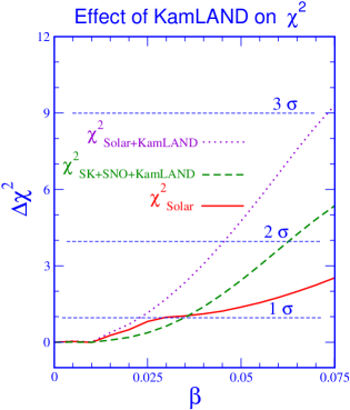
Figure 7: Projection of the global $\Delta\chi^{2}$ function on the fractional fluctuation parameter $\beta$. The solid line represents the calculation using only the solar neutrino data. The dotted line is the calculation when the KamLAND data are included along with the solar neutrino data. For comparison we also show the calculation with solar-neutrino data sensitive only to the ⁸B neutrinos (SK and SNO) combined with the KamLAND data.

In this paper we ignored fluctuations of another kind, namely magnetic field fluctuations impacting neutrino evolution. It has been shown that if neutrinos have sizable magnetic moments they can interact with the transverse magnetic fields spinflavor1 undergoing a spin-flavor precession spinflavor2 . If the magnetic field is noisy the spin-flavor precession will be impacted Loreti:1994ry ; Nicolaidis:da ; Pastor:1995vn ; Nunokawa:1997dp . However a relatively conservative assumption about the maximal size of the solar magnetic field places the spin-flavor resonance at values of $\delta m_{12}^{2}$ Balantekin:dv which is at the region of the neutrino parameter space ruled out by the KamLAND experiment. (For an alternative approach see Ref. Friedland:2002pg ). Hence one can conclude that solar magnetic field fluctuations do not play a role in the solar neutrino physics through the spin-flavor precession mechanism.

We would like to point out that besides in the Sun (and other stars) neutrinos interact with dense matter in several other sites such as the early universe, supernovae, and newly-born neutron stars and neutrino interactions with a stochastic background may play an even more interesting role in those sites Prakash:2001rx . Along those lines a preliminary analysis of the effects of random density fluctuations on matter enhanced neutrino flavor transitions in core-collapse supernovae and implications of such fluctuations for supernova dynamics and nucleosynthesis was given in Ref. Loreti:1995ae .

References

- (1) J. N. Bahcall, M. H. Pinsonneault and S. Basu, Astrophys. J. 555, 990 (2001) [arXiv:astro-ph/0010346].
- (2) A. S. Brun, S. Turck-Chieze and P. Morel, Astrophys. J. 506, 913 (1998) [arXiv:astro-ph/9806272].
- (3) J. Christensen-Dalsgaard, Rev. Mod. Phys. 74, 1073 (2003) [arXiv:astro-ph/0207403].
- (4) J. N. Bahcall, M. H. Pinsonneault, S. Basu and J. Christensen-Dalsgaard, Phys. Rev. Lett. 78, 171 (1997) [arXiv:astro-ph/9610250].
- (5) J. N. Bahcall, S. Basu and M. H. Pinsonneault, Phys. Lett. B 433, 1 (1998) [arXiv:astro-ph/9805135].
- (6) Q. R. Ahmad et al. [SNO Collaboration], Phys. Rev. Lett. 89, 011301 (2002) [arXiv:nucl-ex/0204008].
- (7) J. N. Bahcall, M. C. Gonzalez-Garcia and C. Penya-Garay, arXiv:astro-ph/0212331.
- (8) E. G. Adelberger et al., Rev. Mod. Phys. 70, 1265 (1998) [arXiv:astro-ph/9805121].
- (9) F. N. Loreti and A. B. Balantekin, Phys. Rev. D 50, 4762 (1994) [arXiv:nucl-th/9406003].
- (10) A. B. Balantekin, J. M. Fetter and F. N. Loreti, Phys. Rev. D 54, 3941 (1996) [arXiv:astro-ph/9604061].
- (11) H. Nunokawa, A. Rossi, V. B. Semikoz and J. W. Valle, Nucl. Phys. B 472, 495 (1996) [arXiv:hep-ph/9602307].
- (12) C. P. Burgess and D. Michaud, Annals Phys. 256, 1 (1997) [arXiv:hep-ph/9606295].
- (13) H. Nunokawa, V. B. Semikoz, A. Y. Smirnov and J. W. Valle, Nucl. Phys. B 501, 17 (1997) [arXiv:hep-ph/9701420].
- (14) P. Bamert, C. P. Burgess and D. Michaud, Nucl. Phys. B 513, 319 (1998) [arXiv:hep-ph/9707542].
- (15) E. Torrente-Lujan, Phys. Rev. D 59, 073001 (1999) [arXiv:hep-ph/9807361].
- (16) A. A. Bykov, M. C. Gonzalez-Garcia, C. Pena-Garay, V. Y. Popov and V. B. Semikoz, arXiv:hep-ph/0005244.
- (17) C. Burgess, N. S. Dzhalilov, M. Maltoni, T. I. Rashba, V. B. Semikoz, M. Tortola and J. W. Valle, arXiv:hep-ph/0209094.
- (18) P. Kumar, E. J. Quataert and J. N. Bahcall, Astrophys. J. 458, L83 (1996) [arXiv:astro-ph/9512091].
- (19) S. Couvidat, S. Turck-Chieze and A. G. Kosovichev, arXiv:astro-ph/0203107.
- (20) J. N. Bahcall and P. Kumar, Astrophys. J. 409, L73 (1993) [arXiv:hep-ph/9303229].
- (21) N. S. Dzhalilov and V. B. Semikoz, arXiv:astro-ph/9812149.
- (22) A. B. Balantekin, in Nuclear Physics In The 21st Century: International Nuclear Physics Conference INPC 2001, Berkeley. California (USA), AIP Conference Proceedings, 610, Issue 1, pp. 969-972. arXiv:hep-ph/0109163.
- (23) L. Wolfenstein, Phys. Rev. D 17, 2369 (1978); S. P. Mikheev and A. Y. Smirnov, Sov. J. Nucl. Phys. 42, 913 (1985) [Yad. Fiz. 42, 1441 (1985)]; Nuovo Cim. C 9, 17 (1986).
- (24) A. B. Balantekin, Phys. Rept. 315, 123 (1999) [arXiv:hep-ph/9808281].
- (25) A. B. Balantekin and G. M. Fuller, Phys. Lett. B 471, 195 (1999) [arXiv:hep-ph/9908465].
- (26) T. Ohlsson and H. Snellman, Phys. Lett. B 474, 153 (2000) [arXiv:hep-ph/9912295]; T. Ohlsson and H. Snellman, J. Math. Phys. 41, 2768 (2000) [Erratum-ibid. 42, 2345 (2001)] [arXiv:hep-ph/9910546]; T. Ohlsson and H. Snellman, Eur. Phys. J. C 20, 507 (2001) [arXiv:hep-ph/0103252].
- (27) W. C. Haxton, Phys. Rev. Lett. 57, 1271 (1986), S. J. Parke, Phys. Rev. Lett. 57, 1275 (1986).
- (28) V. Castellani, S. Degl’Innocenti, W. A. Dziembowski, G. Fiorentini and B. Ricci, Nucl. Phys. Proc. Suppl. 70, 301 (1999) [arXiv:astro-ph/9712174].
- (29) A. B. Balantekin and H. Yuksel, J. Phys. G: Nucl. Part. Phys. 29, 665 (2003). [arXiv:hep-ph/0301072].
- (30) B. T. Cleveland et al., Astrophys. J. 496, 505 (1998).
- (31) J. N. Abdurashitov et al. [SAGE Collaboration], J. Exp. Theor. Phys. 95, 181 (2002) [Zh. Eksp. Teor. Fiz. 122, 211 (2002)] [arXiv:astro-ph/0204245].
- (32) W. Hampel et al. [GALLEX Collaboration], Phys. Lett. B 447, 127 (1999).
- (33) M. Altmann et al. [GNO Collaboration], Phys. Lett. B 490, 16 (2000) [arXiv:hep-ex/0006034].
- (34) S. Fukuda et al. [Super-Kamiokande Collaboration], Phys. Rev. Lett. 86, 5651 (2001) [arXiv:hep-ex/0103032], S. Fukuda et al. [Super-Kamiokande Collaboration], Phys. Rev. Lett. 86, 5656 (2001) [arXiv:hep-ex/0103033].
- (35) Q. R. Ahmad et al. [SNO Collaboration], Phys. Rev. Lett. 87, 071301 (2001) [arXiv:nucl-ex/0106015], Q. R. Ahmad et al. [SNO Collaboration], Phys. Rev. Lett. 89, 011302 (2002) [arXiv:nucl-ex/0204009].
- (36) K. Eguchi et al. [KamLAND Collaboration], Phys. Rev. Lett. 90, 021802 (2003) [arXiv:hep-ex/0212021].
- (37) SNO Collaboration, Data Page, http://www.sno.phy.queensu.ca/sno/prlwebpage.
- (38) J. N. Bahcall, M. C. Gonzalez-Garcia and C. Pena-Garay, JHEP 0302, 009 (2003) [arXiv:hep-ph/0212147]; G. L. Fogli, E. Lisi, A. Marrone, D. Montanino, A. Palazzo and A. M. Rotunno, arXiv:hep-ph/0212127, V. Barger and D. Marfatia, Phys. Lett. B 555, 144 (2003) [arXiv:hep-ph/0212126], M. Maltoni, T. Schwetz and J. W. Valle, arXiv:hep-ph/0212129, A. Bandyopadhyay, S. Choubey, R. Gandhi, S. Goswami and D. P. Roy, arXiv:hep-ph/0212146, H. Nunokawa, W. J. Teves and R. Zukanovich Funchal, arXiv:hep-ph/0212202, P. Aliani, V. Antonelli, M. Picariello and E. Torrente-Lujan, arXiv:hep-ph/0212212, P. C. de Holanda and A. Y. Smirnov, arXiv:hep-ph/0212270, A. Ianni, arXiv:hep-ph/0302230, S. M. Bilenky, C. Giunti, J. A. Grifols and E. Masso, arXiv:hep-ph/0211462.
- (39) A. Cisneros, Astrophys. Space Sci. 10, 87 (1971), L. B. Okun, M. B. Voloshin and M. I. Vysotsky, Sov. J. Nucl. Phys. 44, 440 (1986) [Yad. Fiz. 44, 677 (1986)].
- (40) C. S. Lim and W. J. Marciano, Phys. Rev. D 37, 1368 (1988); E. K. Akhmedov, Phys. Lett. B 213, 64 (1988); A. B. Balantekin, P. J. Hatchell and F. Loreti, Phys. Rev. D 41, 3583 (1990); R. S. Raghavan, A. B. Balantekin, F. Loreti, A. J. Baltz, S. Pakvasa and J. Pantaleone, Phys. Rev. D 44, 3786 (1991).
- (41) A. Nicolaidis, Phys. Lett. B 262, 303 (1991).
- (42) S. Pastor, V. B. Semikoz and J. W. Valle, Phys. Lett. B 369, 301 (1996) [arXiv:hep-ph/9509254].
- (43) A. B. Balantekin and F. Loreti, Phys. Rev. D 45, 1059 (1992).
- (44) A. Friedland and A. Gruzinov, arXiv:hep-ph/0202095.
- (45) M. Prakash, J. M. Lattimer, R. F. Sawyer and R. R. Volkas, Ann. Rev. Nucl. Part. Sci. 51, 295 (2001) [arXiv:astro-ph/0103095].
- (46) F. N. Loreti, Y. Z. Qian, G. M. Fuller and A. B. Balantekin, Phys. Rev. D 52, 6664 (1995) [arXiv:astro-ph/9508106].