Yukawa coupling unification and non-universal gaugino mediation of supersymmetry breaking

Abstract:

The requirement of Yukawa coupling unification highly constrains the SUSY parameter space. In several SUSY breaking scenarios it is hard to reconcile Yukawa coupling unification with experimental constraints from $B(b\rightarrow s\gamma)$ and the muon anomalous magnetic moment $a_{\mu}$. We show that $b-\tau$ or even $t-b-\tau$ Yukawa unification can be satisfied simultaneously with $b\rightarrow s\gamma$ and $a_{\mu}$ in the non-universal gaugino mediation scenario. Non-universal gaugino masses naturally appear in higher dimensional grand unified models in which gauge symmetry is broken by orbifold compactification. Relations between SUSY contributions to fermion masses, $b\rightarrow s\gamma$ and $a_{\mu}$ which are typical for models with universal gaugino masses are relaxed. Consequently, these phenomenological constraints can be satisfied simultaneously with a relatively light SUSY spectrum, compared to models with universal gaugino masses.

1 Introduction

Supersymmetric grand unified theories [SUSY GUTs] are well motivated possibilities for physics beyond the standard model [SM]. They provide an explanation of charge assignments of quarks and leptons [1, 2, 3]. Furthermore the unification of gauge couplings in the supersymmetric version of the standard model supports the idea of an underlying theory which unifies three seemingly unrelated gauge symmetries at a scale $M_{G}\sim 2\times 10^{16}$ GeV [4, 5, 6].

There is also a possibility that Yukawa couplings of quarks and leptons unify in a similar way [7]. This is certainly not a necessity since GUT symmetry breaking effects can be incorporated into Yukawa matrices at the GUT scale. Furthermore, each of the MSSM Higgs doublets may originate from more than one unified Higgs representation in which case the relations between Yukawa couplings can be basically arbitrary. (Although given by the underlying theory, these relations might be hard to recover from measurements conducted at low energies.) Nevertheless the hope is that the underlying theory is quite elegant and certain simple relations between Yukawa couplings hold. The simplest and the best motivated relation is the third generation Yukawa coupling unification at the GUT scale: $\lambda_{b}=\lambda_{\tau}$ in SU(5) or $\lambda_{t}=\lambda_{b}=\lambda_{\tau}$ in SO(10).

A precise analysis of gauge and Yukawa coupling unification requires two loop renormalization group running and one loop weak scale SUSY threshold corrections. While gauge coupling unification is not very sensitive to the exact form of SUSY spectrum, the fate of Yukawa coupling unification crucially depends on SUSY threshold corrections [8]. This is due to the fact that gluino and chargino corrections to the bottom quark mass are enhanced by $\tan\beta$ and can naturally be as large as $50\%$. Therefore the success of Yukawa coupling unification strongly depends on the SUSY breaking scenario under consideration. Alternatively, looking at it from the other side, requiring Yukawa coupling unification can point to a preferred SUSY breaking scenario or to a region of the parameter space within each scenario.

Similarly $b\rightarrow s\gamma$ and the anomalous magnetic moment of the muon $a_{\mu}$ receive contributions from SUSY loops. The size of SUSY contributions and their signs depend on the SUSY spectrum. Whether SUSY contributions enhance or suppress these observables compared to the standard model predictions mostly depends on relative signs of the gaugino masses $M_{1}$, $M_{2}$, $M_{3}$ and the $\mu$ term.

For example, in the mSUGRA scenario where all gauginos have the same mass $M_{1/2}$ at $M_{GUT}$, Yukawa coupling unification can be satisfied with negative SUSY threshold corrections to the bottom quark mass. The gluino–sbottom loop is the dominant contribution and is negative for $\mu M_{3}<0$. On the other hand, the chargino contribution to $b\rightarrow s\gamma$ can interfere constructively or destructively with the SM and the charged Higgs contribution. Since the SM and charged Higgs contribution is already somewhat too large, the chargino contribution is expected to lower the branching fraction $B(b\rightarrow s\gamma)$. This happens for $\mu A_{t}<0$, where $A_{t}$ is the top trilinear coupling. The low energy value of $A_{t}$ is related to $-M_{3}$ due to renormalization group [RG] running. Therefore, in order to accommodate the $b\rightarrow s\gamma$ data, $\mu M_{3}>0$ is preferred.  Finally, the SUSY contribution to the anomalous magnetic moment of muon, $a_{\mu}$, is preferred to be positive to comply with the data [9]. The chargino–sneutrino loop is dominant in this case and this contribution is positive for $\mu M_{2}>0$. In conclusion, in the mSUGRA scenario both $b\rightarrow s\gamma$ and $a_{\mu}$ seem to prefer $\mu M_{1/2}>0$ while Yukawa coupling unification strongly prefer $\mu M_{1/2}<0$. This discouraging result led to consideration of Yukawa coupling unification within other well motivated frameworks [10, 11, 13, 14, 15].

In Refs. [10, 11, 12] SO(10) Yukawa unification was considered together with SO(10) motivated boundary conditions for soft SUSY breaking parameters. It was found that $t-b-\tau$ Yukawa unification can be satisfied with positive $\mu$ in a special region where the condition $A_{0}^{2}=4m_{16}^{2}=2m_{10}^{2}$ between universal trilinear coupling ($A_{0}$), universal squark and slepton masses ($m_{16}$) and universal Higgs masses ($m_{10}$) is approximately satisfied. Additional splitting of Higgs masses ($m_{H_{u}}$, $m_{H_{d}}$) at the level of $10\%$ is necessary in order to obtain electroweak symmetry breaking radiatively in large $\tan\beta$ regime and large $m_{16}$ ($>1$ TeV). The reason for Yukawa coupling unification to work in this region is that chargino corrections to the bottom quark mass are enhanced and can dominate the gluino correction, leading to small or even negative total SUSY threshold correction to the bottom quark mass [10]. This region also has other very compelling features. The masses of first two generation scalars are large, the order of $m_{16}$, which suppresses flavor and CP violation (and also proton decay), while the masses of the third generation squarks and sleptons are below 1 TeV keeping this region natural with respect to electroweak symmetry breaking. Although this looks like a drastic departure from mSUGRA scenario, it actually may originate from it when additional RG running above the GUT scale and GUT scale threshold corrections are properly taken into account [10].

In anomaly mediation the gaugino masses $M_{2}$ and $M_{3}$ have opposite signs and so it might be possible to simultaneously achieve negative SUSY threshold correction to the bottom quark mass and positive SUSY contribution to $a_{\mu}$. However in this case the chargino contribution to $b\rightarrow s\gamma$ constructively add to the SM and charged Higgs contribution and thus have to be very suppressed. This is possible only if scalar masses are very heavy (at least few TeV), which is problematic with respect to naturalness constraints [13].

Another approach to accommodate both $b-\tau$ Yukawa coupling unification and constraints from $b\rightarrow s\gamma$ and $a_{\mu}$ was taken up in Ref. [14] where non-universalities in gaugino masses in supergravity models were considered. It was found that Yukawa unification can be achieved with an accuracy of a few percent in significant regions of SUSY parameter space. The corresponding sparticle spectrum is relatively light, consistent with naturalness constraints.

Non-universalities in gaugino masses can be very easily obtained (and are quite generic) in higher dimensional GUT models in which GUT symmetry breaking is achieved by orbifold compactification of extra dimensions. The doublet triplet splitting of Higgs fields is also achieved in an elegant way and proton decay due to dimension 5 operators (which is a serious problem in 4-dimensional GUT models [16]), can be naturally suppressed in these models. The common feature of these models is the existence of a brane or several branes at orbifold fixed points on which the gauge symmetry is restricted to be a subgroup of the GUT symmetry. This results in an effective 4-dimensional theory with gauge symmetry given by an intersection of gauge symmetries on orbifold fixed points [17, 18, 19, 20, 21].

The existence of a brane with restricted gauge symmetry plays an important role in gaugino mediation. If SUSY is broken on a brane with restricted gauge symmetry, non-universal gaugino masses are generated. For example, if using proper boundary conditions $SU(5)$ is broken on a brane down to the SM, non-universal gaugino masses $M_{1},M_{2},M_{3}$ can be generated on this brane [18]. Even more interesting is the situation for $SO(10)$ models in higher dimensions [20, 21] which can contain branes with gauge symmetries being different subgroups of $SO(10)$. Using proper boundary conditions, fixed branes with Pati-Salam $SU(4)\times SU(2)_{L}\times SU(2)_{R}$, Georgi-Glashow $SU(5)\times U(1)$, or flipped $SU(5)^{\prime}\times U(1)^{\prime}$ gauge symmetries can be obtained. If gauginos get masses on these branes, the gauge symmetry relates gaugino masses of the MSSM at the compactification scale. In the case of Pati-Salam gauge symmetry, gaugino masses $M_{2}$ and $M_{3}$ are free parameters while the $M_{1}$ is given by a linear combination of $M_{2}$ and $M_{3}$ [20]. The case of Georgi-Glashow gauge symmetry leads to universal gaugino masses and finally in the case of flipped $SU(5)^{\prime}\times U(1)^{\prime}$ gauge symmetry, $M_{2}=M_{3}$ and $M_{1}$ is an independent parameter [22]. If matter fields are localized on a brane with GUT symmetry Yukawa coupling unification is expected as in four dimensional models.

The compactification scale $M_{c}$ in these models is below (but close to) the GUT scale and the boundary conditions with negligible sfermion masses and trilinear couplings are realized at this scale. Scalar masses and trilinear couplings receive large contributions from gaugino masses through the renormalization group (RG) running between $M_{c}$ and the electroweak (EW) scale. These contributions are flavor blind and therefore the resulting soft SUSY breaking terms at the EW scale cause only a modest flavor violation originating from the Yukawa couplings. 

In the original works on gaugino mediation [24, 25], the compactification scale was assumed to be at or above the GUT scale, in order to preserve the success of gauge coupling unification. Therefore all gaugino masses are equal at $M_{c}$. For $M_{c}=M_{GUT}$, however, this scenario predicts the lightest stau $\tilde{\tau}_{1}$ to be the lightest supersymmetric particle (LSP), which violates cosmological bounds on the existence of stable charged or colored relics from the Big Bang in models which conserve $R$-parity. The situation is different for $M_{c}>M_{GUT}$. In this case additional RG evolution takes place between $M_{c}$ and $M_{GUT}$ [25]. This running generates non-vanishing scalar masses and trilinear couplings at the GUT scale. Most importantly, the stau mass receives a positive contribution which eventually can make the $\tilde{\tau}_{1}$ heavier than the lightest neutralino $\widetilde{Z}_{1}$. This removes the unpleasant charged LSP feature of the scenario with $M_{c}=M_{GUT}~{}$[25, 26].

This cure of the stau LSP problem doesn’t apply to the case of non-universal case (in which $M_{c}<M_{GUT}$). However, in this case the non-universal gaugino masses help us to obtain viable SUSY spectra with a neutralino LSP, at least in some regions of model parameter space. A recent study [27] of the non-universal gaugino mediation scenario delineates the allowed regions of the SUSY parameter space consistent with neutralino LSP and constraints from $b\rightarrow s\gamma$ and $a_{\mu}$ for various boundary conditions on gaugino masses.

In this paper we study to which extent Yukawa coupling unification can be satisfied together with phenomenological constraints from $b\rightarrow s\gamma$ and $a_{\mu}$ in the non-universal gaugino mediation scenario. In Sec. 2 we present basic results of non-universal gaugino mediation and obtain approximate formulas for gaugino, squark and slepton masses. In Sec. 3 we study SUSY threshold corrections to the bottom quark mass based on the SUSY spectrum. Understanding of threshold corrections helps us to understand numerical results presented in Sec. 4. The summary of our results and our conclusions are given in Sec. 5.

2 SUSY spectrum of non-universal gaugino mediation

Gaugino mediated SUSY breaking is quite economical. In the non-universal scenario this mechanism is parametrized by three soft SUSY breaking gaugino masses at the compactification scale $M_{c}$: $M_{a}(M_{c})$, $a=1,2,3$. Depending on the localization of the Higgs fields, soft SUSY breaking Higgs masses and the $\mu$–term can also be generated. Soft SUSY breaking masses of squarks and sleptons and trilinear couplings are negligible at $M_{c}$. More details on possible models are presented in Ref. [27] and references therein.

It is an useful exercise to obtain approximate analytic formulas of the SUSY spectrum. These will help us in understanding of SUSY threshold corrections to the bottom quark mass and thus the region of SUSY parameter space where Yukawa coupling unification can be satisfied. The complete set of two loop MSSM RG evolution equations [RGEs] can be find in [28]. In this section, we use one loop RGEs for the gauge couplings, the gaugino masses and the scalar masses. We neglect the contribution of scalar masses and trilinear couplings in the running.

From the one loop RGEs for gaugino masses and gauge couplings,

$$\frac{dM_{a}}{d\log\mu} = 2C_{a}g_{a}^{2}M_{a},\quad C_{a}=\frac{1}{16\pi^{2}}(33/5,1,-3),\quad a=1,2,3$$ (1)

$$\frac{dg_{a}}{d\log\mu} = C_{a}g_{a}^{3},$$ (2)

we obtain the well known result that gaugino masses scale with the square of gauge couplings:

$$\frac{M_{a}(\mu)}{g_{a}^{2}(\mu)}\;=\;const\;=\;\frac{M_{a}(M_{c})}{g^{2}},$$ (3)

where $g$ is the gauge coupling constant at $M_{c}$. Using weak scale values: $\alpha_{3}(M_{Z})=0.118$, $\alpha_{em}(M_{Z})=1/128$, $\sin^{2}\theta_{W}=0.22$, $\alpha_{2}=\alpha_{em}/\sin^{2}\theta_{W}\sim 0.035$, $\alpha_{1}=(5/3)\alpha_{em}/cos^{2}\theta_{W}\sim 0.017$, and the GUT scale value of the gauge coupling, $\alpha_{G}=g^{2}/4\pi\sim 0.04$, it is easy to find weak scale values of gaugino masses:

$$M_{1}(M_{Z}) \sim 0.4\,M_{1},$$ (4)

$$M_{2}(M_{Z}) \sim 0.9\,M_{2},$$ (5)

$$M_{3}(M_{Z}) \sim 3.0\,M_{3}.$$ (6)

Similarly, one loop RGEs of squarks and sleptons are given by

$$\frac{dm_{\tilde{f}}^{2}}{d\log\mu}\;=\;\frac{1}{16\pi^{2}}\,\beta_{m^{2}_{\tilde{f}}},$$ (7)

with

$$\beta_{m^{2}_{Q}} = -\frac{32}{3}g_{3}^{2}M_{3}^{2}\,-\,6g_{2}^{2}M_{2}^{2}\,-\,\frac{2}{15}g_{1}^{2}M_{1}^{2}\,+\,\dots,$$

$$\beta_{m^{2}_{U}} = -\frac{32}{3}g_{3}^{2}M_{3}^{2}\,-\,\frac{32}{15}g_{1}^{2}M_{1}^{2}\,+\,\dots,$$

$$\beta_{m^{2}_{D}} = -\frac{32}{3}g_{3}^{2}M_{3}^{2}\,-\,\frac{8}{15}g_{1}^{2}M_{1}^{2}\,+\,\dots,$$

$$\beta_{m^{2}_{L}} = -6g_{2}^{2}M_{2}^{2}\,-\,\frac{6}{5}g_{1}^{2}M_{1}^{2}\,+\,\dots,$$

$$\beta_{m^{2}_{E}} = \,-\,\frac{24}{5}g_{1}^{2}M_{1}^{2}\,+\,\dots,$$

where dots represent terms which are zero at $M_{c}$, being proportional to scalar masses and trilinear couplings. For comparable values of gaugino masses we can neglect contributions from terms proportional to $M_{1}$ (except in the case of right handed sleptons) since these are suppressed compared to terms proportional to $M_{2}$ and $M_{3}$ by smaller value of gauge coupling $g_{1}$ and also the group theoretical factors.

In this approximation the solution can be written as:

$$m^{2}_{Q}(\mu) = \frac{8}{9}M_{3}^{2}\left[\left(\frac{g_{3}(\mu)}{g}\right)^{4}-1\right]\,+\,\frac{3}{2}M_{2}^{2}\left[1-\left(\frac{g_{2}(\mu)}{g}\right)^{4}\right],$$ (8)

$$m^{2}_{U}(\mu) = \frac{8}{9}M_{3}^{2}\left[\left(\frac{g_{3}(\mu)}{g}\right)^{4}-1\right],$$ (9)

$$m^{2}_{D}(\mu) = \frac{8}{9}M_{3}^{2}\left[\left(\frac{g_{3}(\mu)}{g}\right)^{4}-1\right],$$ (10)

$$m^{2}_{L}(\mu) = \frac{3}{2}M_{2}^{2}\left[1-\left(\frac{g_{2}(\mu)}{g}\right)^{4}\right],$$ (11)

$$m^{2}_{E}(\mu) = \frac{2}{11}M_{1}^{2}\left[1-\left(\frac{g_{1}(\mu)}{g}\right)^{4}\right],$$ (12)

and for the weak scale values we obtain:

$$m_{Q}(M_{Z}) = 2.6\,M_{3}\,\left[1+0.03\left(\frac{M_{2}}{M_{3}}\right)^{2}\right],$$ (13)

$$m_{U}(M_{Z}) = m_{D}(M_{Z})\;=\;2.6\,M_{3},$$ (14)

$$m_{L}(M_{Z}) = 0.6\,M_{2},$$ (15)

$$m_{E}(M_{Z}) = 0.39\,M_{1}.$$ (16)

We also need to estimate the top trilinear coupling which enters the chargino contribution to the bottom quark mass. The one loop RGE is given by

$$\frac{dA_{t}}{d\log\mu}\;=\;\frac{1}{16\pi^{2}}\,\beta_{A_{t}},$$ (17)

where

$$\beta_{A_{t}}=\frac{32}{3}g_{3}^{2}M_{3}\,+\,6g_{2}^{2}M_{2}\,+\,\frac{26}{15}g_{1}^{2}M_{1}\,+\,\dots\,.$$ (18)

In the same approximation as for the squarks and sleptons, we obtain

$$A_{t}(\mu)=\frac{16}{9}M_{3}\left[1-\left(\frac{g_{3}(\mu)}{g}\right)^{2}\right]\,-\,3M_{2}\left[1-\left(\frac{g_{2}(\mu)}{g}\right)^{2}\right],$$ (19)

and the weak scale value is given by

$$A_{t}(M_{Z})=-3.5\,M_{3}\,-0.4M_{2}.$$ (20)

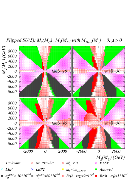
Figure 1: Typical parameter space slices of flipped SU(5) gaugino mediation models. Areas hatched in red are excluded by the presence of tachyonic particles or by the lack of radiative EW symmetry breaking. The magenta areas represent regions with stau LSPs. Blue and yellow areas are excluded by LEP.

These results for gaugino, squark and slepton masses should be interpreted with care. However the approximation used is precise enough to point out the main features of the SUSY spectrum in non-universal gaugino mediation. First of all, from Eqs. (4) and (16) we immediately see the well-known problem associated with gaugino mediation, the stau being LSP. Neither the bino nor the right-handed stau are mass eigenstates however. The lightest neutralino is a mixture of gauginos and Higgsinos, and for $\tilde{\tau}_{1}$ the D-terms as well as left-right mixing have to be properly taken into account. In result, there is quite significant region of parameter space with neutralino LSP, as illustrated by Fig. 1. The allowed region opens up with increasing $M_{1}$, either because of the large portion of Higgsino in the lightest neutralino (along the line where electroweak symmetry breaking is possible, where the $\mu$ term is small) or the large portion of wino in the lightest neutralino (for small values of $M_{2}$ compared to $M_{1}$). On the other hand with increasing $\tan\beta$ the $\tau$ Yukawa coupling also increases and the terms proportional to Yukawa couplings in RG equations become more important. These terms suppress the stau mass and so the allowed region is shrinking. For more results and discussion see Ref. [27].

The second important observation is that the gluino, stop and sbottom masses are very close to each other and approximately equal to $3M_{3}$. This will be crucial for discussion of SUSY threshold corrections to the bottom quark mass in the following section.

3 SUSY threshold corrections to the bottom quark mass

The dominant corrections to the bottom quark mass come from gluino-sbottom and chargino-stop diagrams. Pieces proportional to $\tan\beta$ can be approximated by:

$$\left(\frac{\delta m_{b}}{m_{b}}\right)^{\tilde{g}}\sim\;\frac{2\alpha_{3}}{3\pi}\;\mu\tan\beta\;\frac{m_{\tilde{g}}}{M_{SUSY}^{2}}$$ (21)

and

$$\left(\frac{\delta m_{b}}{m_{b}}\right)^{\tilde{\chi}^{\pm}}\sim\;\frac{\lambda^{2}_{t}}{16\pi^{2}}A_{t}\,\tan\beta\;\frac{\mu}{M_{SUSY}^{2}}.$$ (22)

Here $M_{SUSY}$ is the typical mass of particles in the corresponding loop. In the previous section we found that

$$M_{SUSY} \sim m_{\tilde{g}}\,\sim\,m_{\tilde{b}}\,\sim\,m_{\tilde{t}}\,\sim\,3M_{3},$$ (23)

$$A_{t} \sim -3.5M_{3}\,-0.4M_{2}.$$

Taking $\alpha_{3}(M_{Z})=0.118$ and $\lambda_{t}(M_{Z})\sim 1$, we can obtain very simple formulas for the SUSY threshold corrections to $m_{b}$:

$$\left(\frac{\delta m_{b}}{m_{b}}\right)^{\tilde{g}} \sim \frac{1}{100M_{3}}\;\mu\tan\beta,$$ (24)

$$\left(\frac{\delta m_{b}}{m_{b}}\right)^{\tilde{\chi}^{\pm}} \sim -\frac{1}{500M_{3}}\left(1+\frac{1}{9}\frac{M_{2}}{M_{3}}\right)\mu\tan\beta.$$ (25)

Comparing the last two expressions we find

$$\left(\frac{\delta m_{b}}{m_{b}}\right)^{\tilde{\chi}^{\pm}}\sim-\frac{1}{5}\left(\frac{\delta m_{b}}{m_{b}}\right)^{\tilde{g}}\left(1+\frac{1}{9}\frac{M_{2}}{M_{3}}\right).$$ (26)

Clearly, the gluino corrections will dominate unless $M_{2}\sim 40M_{3}$. So for positive $\mu$, the Yukawa unification can be expected only for negative $M_{3}$, and the dependance on $M_{2}$ and $M_{1}$ is not expected to be significant. The results shown in the figures of the next section are in agreement with these findings. Although $\mu M_{3}<0$ is strongly preferred as in the mSUGRA scenario, non-universal gaugino masses can help to satisfy constraints from $b\rightarrow s\gamma$ and $a_{\mu}$ in some portion of SUSY parameter space.

4 Yukawa coupling unification

In this section, we present results of our numerical analysis. There are several programs readily available for numerically solving the necessary, coupled system of RGEs at the two-loop level. The most popular ones are ISAJET [29], SoftSUSY [30], Spheno [31] and Suspect [32]. Recently, a satisfactory agreement was demonstrated between the latest versions of these codes [33]. To calculate the sparticle spectrum and the Yukawa couplings between $M_{c}$ and the weak scale, we use ISAJET version 7.64. The calculational procedure implemented in ISAJET, with special emphasis on Yukawa couplings and the theoretical uncertainties in their determination, is described in a recent publication [12]. Due to the known theoretical uncertainties, we treat our numerical results with a reasonable flexibility, and conclude that unification takes place when the GUT scale Yukawas agree within a few percent. For the evaluation of the branching fraction $B(b\rightarrow s\gamma)$ and the muon anomalous magnetic moment $a_{\mu}$, we use the calculations presented in Refs. [34] and [35], respectively.

In our plots, we present theoretically, phenomenologically and experimentally acceptable models. We discard models with tachyonic particles, no radiative EW symmetry breaking [REWSB] or a stau LSP as unacceptable. We further require that the $Z$ boson have negligible decay rates to sparticles and also impose the following LEP2 constraints on the weak scale masses of the lightest gauginos ($\widetilde{Z}_{1}$, $\widetilde{W}_{1}$), sleptons ($\tilde{e}_{1}$,$\tilde{\mu}_{1}$,$\tilde{\tau}_{1}$) and Higgs boson [36]:

$$m_{\widetilde{Z}_{1}}>37~{}{\rm GeV},~{}~{}m_{\widetilde{W}_{1}}>100~{}{\rm GeV},$$

$$m_{\tilde{e}_{1}}>92~{}{\rm GeV},~{}~{}m_{\tilde{\mu}_{1}}>85~{}{\rm GeV},~{}~{}m_{\tilde{\tau}_{1}}>68~{}{\rm GeV},$$ (27)

$$m_{h}>91~{}{\rm GeV}.$$

Models that do not satisfy the above criteria are excluded from our study. Models passing all the above criteria are further analyzed with respect to the indirect experimental constraints from $B(b\rightarrow s\gamma)$ and $a_{\mu}$. We impose the following limits:

$$-10<a_{\mu}\times 10^{10}<60,~{}~{}~{}{\rm and}~{}~{}~{}2<B(b\rightarrow s\gamma)\times 10^{4}<5.$$ (28)

These limits correspond to the experimentally allowed regions approximately at 2$\sigma$ [37]. In our plots, we color models that do not satisfy this $B(b\rightarrow s\gamma)$ (or $a_{\mu}$) constraint by shades of red (or gray). Models that pass all the above requirements are marked by green on our figures.

As discussed earlier, for gaugino mediation only the gaugino and Higgs masses are non-zero at $M_{c}$. In our numerical analysis we assume $M_{c}=10^{16}$ GeV. The rest of the soft breaking parameters, namely all squark and slepton masses and trilinear couplings are assumed to vanish at $M_{c}$. The only other remaining free model parameter is $\tan\beta$, since our requirement of the REWSB fixes the rest of the Higgs sector. Since we scan through both positive and negative values of gaugino masses, the sign of $\mu$ is not an independent parameter and we present results only for $\mu>0$.  Thus, the parameter space of the non-universal gaugino mediation scenario is spanned by six parameters:

$$M_{1}(M_{c}),~{}~{}M_{2}(M_{c}),~{}~{}M_{3}(M_{c}),~{}~{}M_{H_{u}}(M_{c}),~{}~{}M_{H_{d}}(M_{c})~{}~{}{\rm and}~{}~{}\tan\beta.$$ (29)

This corresponds to the case when gaugino masses are generated on a brane with SM gauge symmetry. If SUSY breaking happens on a brane with larger gauge symmetry, gaugino masses are further restricted [20]. In the case Pati-Salam symmetry gaugino masses satisfy

$$M_{1}={3\over 5}M_{2}+{2\over 5}M_{3},$$ (30)

and in the case of flipped SU(5)

$$M_{2}=M_{3}.$$ (31)

In what follows we present results for $b-\tau$ and $t-b-\tau$ Yukawa coupling unification in the SM scenario and the flipped SU(5) scenario. In both cases we also show results for vanishing Higgs masses, $M_{H_{u}}(M_{c})=M_{H_{d}}(M_{c})=0$. Finally, we briefly comment on the Pati-Salam scenario.

4.1 Bottom - tau Yukawa unification with independent gaugino masses

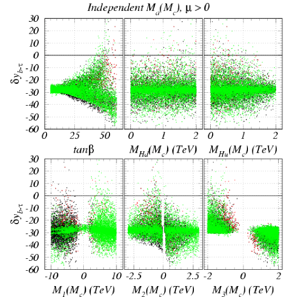
Figure 2: A scan of the full parameter space with independent gaugino and Higgs masses at $M_{c}$ and $\mu>0$. The variable $\delta y_{b-\tau}$, defined in Eq.(32), is plot versus the model parameters. Black (red) dots mark models that deviate from the central value of the $a_{\mu}$ ($B(b\rightarrow s\gamma)$) measurement by 2$\sigma$. Models marked by green dots satisfy all our constraints.

To quantify the amount of $b-\tau$ unification, we use the variable

$$\delta y_{b-\tau}=100\left(\frac{y_{b}}{y_{\tau}}-1\right),$$ (32)

where $y_{b}$ and $y_{\tau}$ are the values of the $b$ and $\tau$ Yukawa couplings at the compactification scale. The factor 100 is introduced so that $\delta y_{b-\tau}$ measures the amount of percentage deviation from perfect unification.

To find the regions with the best Yukawa unification, namely regions with $\delta y_{b-\tau}\sim 0$, we scan the full parameter space as indicated by Eq.(29). Fig. 2 shows the parameter ranges and the result of such a random scan. Here, we plot $\delta y_{b-\tau}$ versus the free parameters of the model for $\mu>0$. We observe two branches of models, differentiated by the sign of $M_{3}$. As expected from the inspection of the SUSY threshold corrections in Sec. 3, the branch with negative $M_{3}$ unifies the $b$ and $\tau$ Yukawa couplings while the other does not. Yukawa unification happens in relatively wide parameter ranges. But models that simultaneously comply with unification and the indirect experimental constraints are confined close to $\tan\beta\sim 45$, $M_{1}(M_{c})\stackrel{{\scriptstyle>}}{{\sim}}2$ TeV, –2 TeV $\lesssim M_{2}(M_{c})\lesssim 1$ TeV, and $M_{3}(M_{c})\lesssim-1$ TeV. In contrast, there is no strong preference for particular values of Higgs masses, except perhaps for low $M_{H_{u}}$ values. This latter fact is supported by an independent scan with vanishing Higgs masses $M_{h_{u}}(M_{c})=M_{h_{d}}(M_{c})=0$, shown in Fig. 3. For this case $b-\tau$ unification occurs in similar ranges as for non-zero Higgs masses.

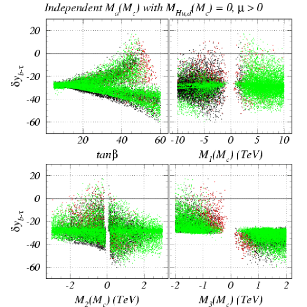
Figure 3: Same as Fig. 2 except with vanishing Higgs masses at $M_{c}$.

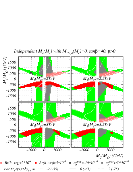
Figure 4: Yukawa unification contours in the $M_{3}$ versus $M_{2}$ plane for independent gaugino and vanishing Higgs masses at $M_{c}$. We chose $\tan\beta=40$ and $\mu>0$.

Figs. 2 and 3 point to specific regions of the parameter space where Yukawa unification is achieved and the constraints on $B(b\rightarrow s\gamma)$ and $a_{\mu}$ are satisfied simultaneously. To explore this parameter region further, we fix $\tan\beta=40$ and scan the $M_{2}$ versus $M_{3}$ planes for fixed values of $M_{1}$. Fig. 4 shows the results of these scans. White areas are theoretically unacceptable and areas colored by shades of red (gray) are excluded by $B(b\rightarrow s\gamma)$ ($a_{\mu}$). Green areas are allowed by all the constraints. As expected, in the negative $M_{2}$ and $M_{3}$ quadrants there are large regions with good Yukawa unification. For $M_{1}>2$ TeV significant parts of these regions are allowed both by $b\rightarrow s\gamma$ and $a_{\mu}$. Thus, Fig. 4 clearly demonstrates that, for the case of independent gaugino and vanishing Higgs masses, there exist parts of the parameter space where it is possible to reconcile $b-\tau$ unification with all the considered constraints.

4.2 Top - bottom - tau Yukawa unification with independent gaugino masses

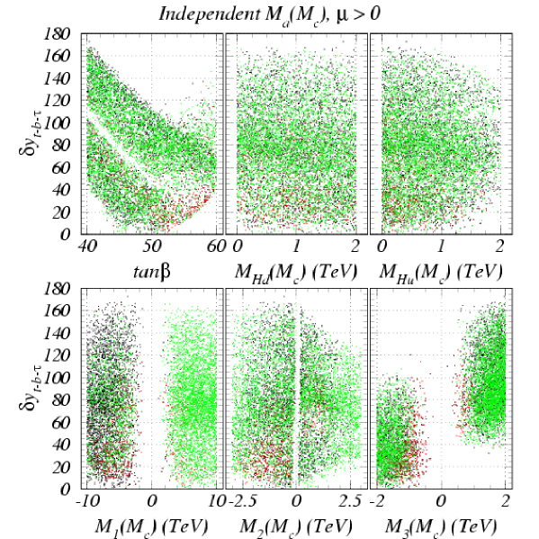
Figure 5: A scan of the relevant parameter space with independent gaugino and Higgs masses at $M_{c}$ and $\mu>0$. The variable $\delta y_{t-b-\tau}$ is plot vs. the model parameters. Black (red) dots mark models that deviate from the central value of the $a_{\mu}$ ($B(b\rightarrow s\gamma)$) measurement by 2$\sigma$. Models marked by green dots satisfy all our constraints.

To gauge the amount of $t-b-\tau$ unification, similarly to Eq.(32), we define

$$\delta y_{t-b-\tau}=100\left(\frac{\max(y_{t},y_{b},y_{\tau})}{\min(y_{t},y_{b},y_{\tau})}-1\right),$$ (33)

where $y_{x}$ are the values of the $t$, $b$ and $\tau$ Yukawa couplings at $M_{c}$. Notice that unlike $\delta y_{b-\tau}$, $\delta y_{t-b-\tau}$ never becomes negative. In Fig. 5, we plot $\delta y_{t-b-\tau}$ versus the relevant parameters from a scan for $\mu>0$ in the high $\tan\beta$ region where Yukawa unification is expected. Again, we find models with good unification satisfying all the constraints. The conclusion is similar to that of the $b-\tau$ unification case. Provided that we allow high enough $|M_{1}(M_{c})|$ values, unification is achieved at moderate values of $M_{2}$ and $M_{3}$. Since the correlation between $\delta y_{t-b-\tau}$ and the Higgs masses seems to be weak just like in the case of $\delta y_{b-\tau}$, we conducted a similar scan for $M_{h_{u}}(M_{c})=M_{h_{d}}(M_{c})=0$. The results are shown by Fig. 6. In a considerable part of the parameter space, we find well unified models consistent with all other constraints.

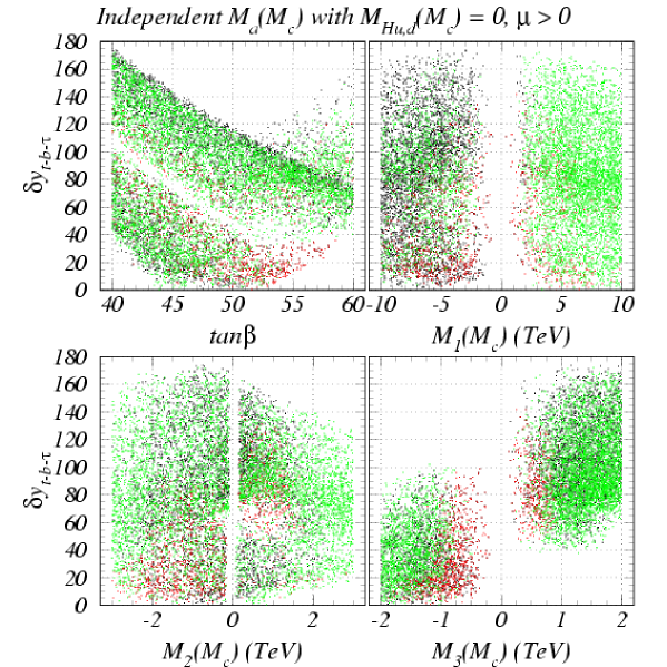
Figure 6: Same as Fig. 5 except with vanishing Higgs masses at the compactification scale.

Both Fig. 5 and Fig. 6 show that Yukawa unification is achieved for two narrow regions of $\tan\beta$, namely 45 and 50. These two regions are correlated with the sign of $M_{2}$. The region with $\tan\beta\sim 45$ corresponds to $M_{2}>0$ while the region with $\tan\beta\sim 50$ corresponds to $M_{2}<0$. This can be seen on Fig. 7, where we present contours of $t-b-\tau$ unification down to 5%. This plot illustrates for $\tan\beta=45$ that with vanishing Higgs masses and $M_{1}\sim 5-7$ TeV there are significant regions of the $M_{2}$-$M_{3}$ parameter plane where $t-b-\tau$ unification takes place. In particular, Yukawas unify for $M_{2}>0$. A similar plot, which we do not include here, for $\tan\beta=50$ reveals $t-b-\tau$ unification for $M_{2}<0$.

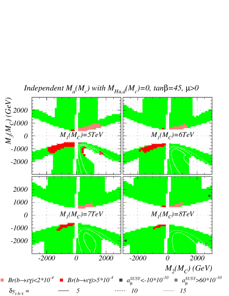
Figure 7: Same as Fig. 4 with contours of $t-b-\tau$ Yukawa unification being shown. On this plot $\tan\beta=45$.

In order to illustrate typical sparticle spectra for models with good unification, we show a few parameters for selected models in Table 1. The firs two models have non-vanishing Higgs masses and the third model has zero Higgs masses at the compactification scale. We find that well unified models typically have the lightest gauginos in the few hundred GeV mass range, lightest sleptons and Higgses below 1 TeV, and the lightest squarks in the TeV range. This sort of spectrum may allow the Tevatron to cover a limited part of the parameter space, while the LHC has a chance to produce several types of sparticles. A LC, depending on its center of mass energy and the actual model parameters, may produce only the lightest Higgs boson or additionally the lightest gauginos and sleptons.

As Table 1 illustrates, the lightest neutralino is always almost degenerate with the lightest chargino, that is it always has a strong wino admixture. As a consequence, in this model the neutralino relic abundance is generally much lower than the experimental value of the cold dark matter [38], as it was pointed out in [27].

4.3 More constrained cases

Results for independent gaugino masses indicate that Yukawa unification happens for a wide range of $M_{2}$, which suggests that it can be achieved also in the case of gaugino masses being restricted by flipped SU(5) symmetry (cf. Eq. (31)). Motivated by this, we re-scan the full parameter space with $M_{2}=M_{3}$ and find that the results are qualitatively very similar to those of independent gaugino masses, both in the $b-\tau$ and $t-b-\tau$ cases. For completeness, we present results for $t-b-\tau$ Yukawa unification in Fig. 8. This is a scan with independent Higgs masses although these are not showed in the figure since there is no preference for particular values of Higgs masse just as in previous cases. As expected, only solutions with $\tan\beta\sim 50$ are found in this case. We also performed a scan with vanishing Higgs masses with similar results. It is interesting to note that even in this case, when the SUSY breaking scenario is characterized by just three soft SUSY breaking parameters: $M_{1},M_{2}=M_{3}$ and $\tan\beta$, we find a region with good Yukawa unification as well as $b\rightarrow s\gamma$ and $a_{\mu}$. In this case Yukawa unification is achieved at slightly higher values of gaugino masses compared to the scenario with independent gaugino masses: $M_{3}\lesssim 1.5$ TeV, $M_{1}\stackrel{{\scriptstyle>}}{{\sim}}6$ TeV. Typical SUSY spectra from this region are represented by model 4 in Table 1. The spectrum in this case exhibits similar features as spectra for independent gaugino masses.

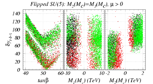
Figure 8: A scan of the relevant parameter space with flipped SU(5) related gaugino masses at $M_{c}$ and $\mu>0$. The variable $\delta y_{t-b-\tau}$ is plot vs. the model parameters. Black (red) dots mark models that deviate from the central value of the $a_{\mu}$ ($B(b\rightarrow s\gamma)$) measurement by 2$\sigma$. Models marked by green dots satisfy all our constraints.

Finally, in the case with gaugino masses constrained by Pati-Salam symmetry (30), we do not expect Yukawa unification while keeping a relatively light SUSY spectrum. Based on results for independent gaugino masses and the flipped SU(5) case we see that $|M_{1}|\gg|M_{2}|$ is highly preferred. However, this can be only achieved for large values of $M_{3}$. Therefore Yukawa unification in this case might only be satisfied with gluino and squarks not lighter than several TeV which makes this scenario phenomenologically less interesting.

model	1	2	3	4
$M_{1}(M_{c})$	3929.6	3778.4	4596.2	6360.3
$M_{2}(M_{c})$	481.3	777.9	959.5	-1613.7
$M_{3}(M_{c})$	-1532.9	-866.9	-1989.5	-1613.7
$M_{H_{u}}(M_{c})$	950.7	816.1	0.0	996.9
$M_{H_{d}}(M_{c})$	144.9	58.8	0.0	138.9
$\tan\beta$	45.2	44.7	44.4	51.1
$f_{t}(M_{GUT})$	0.525	0.516	0.524	0.509
$f_{b}(M_{GUT})$	0.522	0.510	0.507	0.507
$f_{\tau}(M_{GUT})$	0.525	0.532	0.519	0.488
$\delta_{b-\tau}$	-0.6	-4.1	-2.2	4.0
$\delta_{t-b-\tau}$	0.6	4.3	3.3	4.3
$m_{\tilde{g}}$	3376.6	1986.8	4325.5	3545.0
$m_{\tilde{u}_{L}}$	2837.5	1738.1	3647.0	3104.6
$m_{\tilde{d}_{R}}$	2864.7	1721.4	3642.8	3044.4
$m_{\tilde{t}_{1}}$	2500.1	1494.5	3231.9	2649.5
$m_{\tilde{b}_{1}}$	2484.0	1454.2	3216.9	2585.9
$m_{\tilde{e}_{L}}$	765.6	845.9	1036.9	1532.4
$m_{\tilde{e}_{R}}$	1460.5	1402.3	1688.8	2343.8
$m_{\tilde{\nu}_{e}}$	761.4	842.1	1033.8	1530.3
$m_{\tilde{\tau}_{1}}$	615.9	680.6	911.6	1357.3
$m_{\tilde{\nu}_{\tau}}$	622.5	679.8	919.7	1357.3
$m_{\widetilde{W}_{1}}$	434.3	640.8	837.9	1283.6
$m_{\widetilde{Z}_{2}}$	1610.1	823.0	2063.1	1542.8
$m_{\widetilde{Z}_{1}}$	434.1	640.4	837.7	1283.4
$m_{h}$	122.5	119.6	123.1	123.4
$m_{A}$	843.9	659.3	628.2	877.5
$m_{H^{+}}$	849.9	666.5	635.9	883.9
$\mu$	1734.7	875.7	2253.8	1661.9
$a_{\mu}\times 10^{10}$	35.99	48.21	18.50	8.04
$B(b\rightarrow s\gamma)\times 10^{4}$	3.78	3.65	3.96	4.33

Table 1: Representative model parameters, and (s)particle masses (in GeVs) for models with good Yukawa unification.

5 Summary and conclusions

In this work, we analysed Yukawa unification in models with non-universal gaugino mediation of SUSY breaking. We assumed that all soft SUSY breaking terms vanish at the compactification scale $M_{c}$ (which is set slightly below the usual SUSY GUT scale). The exception being the gaugino and Higgs masses, which were assumed to be non-zero and independent at $M_{c}$. We also considered the cases with vanishing Higgs masses and degenerate $M_{2}$ and $M_{3}$ values.

We showed that $b-\tau$, and even $t-b-\tau$, unification can be satisfied simultaneously with experimental constraints on $b\rightarrow s\gamma$ and $a_{\mu}$. This typically happens for $|M_{1}|\gg|M_{2}|,|M_{3}|$. The large values of $M_{1}$ are needed in order to have a neutralino LSP in a substantial part of the parameter space. This is necessary especially in the large $\tan\beta$ region where Yukawa unification can be achieved.

Yukawa unification strongly prefers $\mu M_{3}<0$ just as the mSUGRA scenario or SO(10) motivated models [10, 11, 12]. The advantage of non-universal gaugino mediation is the possibility of achieving Yukawa coupling unification with a relatively light spectrum. This, on the other hand, provides a sizeable SUSY contribution to the muon anomalous magnetic moment (shown by Table 1), while the SUSY contribution to $a_{\mu}$ in most of other scenarios is negligible [10, 11, 13, 12]. The relic density of neutralinos from resulting region of SUSY parameter space is typically below the expectations from cosmological observations. For recent discussion of neutralino relic density in other frameworks for Yukawa coupling unification, see Refs. [12, 39, 40, 41].

References

-
[1]
J. Pati and A. Salam, Phys. Rev. D 8 (1973) 1240;
J. Pati and A. Salam, Phys. Rev. D 10 (1974) 275. - [2] H. Georgi and S. Glashow, Phys. Rev. Lett. 32 (1974) 438.
-
[3]
H. Georgi, Particles and Fields, Proceedings of the APS Div.
of Particles and Fields, ed C. Carlson, p. 575 (1975);
H. Fritzsch and P. Minkowski, Ann. Phys. 93, (1975) 193. -
[4]
H. Georgi, H.R. Quinn and S. Weinberg, Phys. Rev. Lett. 33 (1974) 451;
S. Weinberg, Phys. Lett. B 91 (1980) 51. -
[5]
S. Dimopoulos, S. Raby and F. Wilczek, Phys. Rev. D 24 (1981) 1681;
S. Dimopoulos and H. Georgi, Nucl. Phys. B 193 (1981) 150;
L. Ibanez and G.G. Ross, Phys. Lett. B 105 (1981) 439;
N. Sakai, Z. Physik C 11 (1981) 153;
M.B. Einhorn and D.R.T. Jones, Nucl. Phys. B 196 (1982) 475;
W.J. Marciano and G. Senjanovic, Phys. Rev. D 25 (1982) 3092. -
[6]
U. Amaldi, W. de Boer and H. Fürstenau, Phys. Lett. B 260 (1991) 447;
J. Ellis, S. Kelly and D.V. Nanopoulos, Phys. Lett. B 260 (1991) 131;
P. Langacker and M. Luo, Phys. Rev. D 44 (1991) 817. -
[7]
For early discussion of fermion masses in grand unified theories, see
T. Banks, Nucl. Phys. B 303 (1988) 172;
M. Olechowski and S. Pokorski, Phys. Lett. B 214 (1988) 393;
S. Pokorski, Nucl. Phys. B 13 (1990) 606 (Proc. Supp.);
B. Ananthanarayan, G. Lazarides and Q. Shafi, Phys. Rev. D 44 (1991) 1613;
Q. Shafi and B. Ananthanarayan, ICTP Summer School lectures (1991);
S. Dimopoulos, L.J. Hall and S. Raby, Phys. Rev. Lett. 68 (1992) 1984;
ibid Phys. Rev. D 45 (1992) 4192;
G. Anderson et al., Phys. Rev. D 47 (1993) 3702;
B. Ananthanarayan, G. Lazarides and Q. Shafi, Phys. Lett. B 300 (1993) 245;
G. Anderson et al., Phys. Rev. D 49 (1994) 3660;
B. Ananthanarayan, Q. Shafi and X.M. Wang, Phys. Rev. D 50 (1994) 5980. -
[8]
L.J. Hall, R. Rattazzi and U. Sarid, Phys. Rev. D 50 (1994) 7048;
R. Hempfling, Phys. Rev. D 49 (1994) 6168;
M. Carena, M. Olechowski, S. Pokorski and C. E. Wagner, Nucl. Phys. B 426 (1994) 269;
T. Blazek, S. Pokorski and S. Raby, Phys. Rev. D 52 (1995) 4151;
R. Rattazzi and U. Sarid, Phys. Rev. D 53 (1996) 1553;
D. M. Pierce, J. A. Bagger, K. T. Matchev and R. J. Zhang, Nucl. Phys. B 491 (1997) 3. -
[9]
H.N. Brown et al., Phys. Rev. Lett. 86 (2001) 2227;
U. Chattopadhyay and P. Nath, Phys. Rev. D 53 (1996) 1648. -
[10]
T. Blažek, R. Dermíšek and S. Raby, Phys. Rev. Lett. 88 (2002) 111804;
ibid Phys. Rev. D 65 (2002) 115004;
S. Raby, talk presented at SUSY 2001, Dubna, Russia, June 2001, hep-ph/0110203;
R. Dermíšek, talk presented at SUSY 2001, Dubna, Russia, June 2001, hep-ph/0108249. -
[11]
H. Baer, M. Diaz, J. Ferrandis and X. Tata, Phys. Rev. D 61 (2000) 111701;
H. Baer and J. Ferrandis, Phys. Rev. Lett. 87 (2001) 211803. - [12] D. Auto, H. Baer, C. Balázs, A. Belyaev, J. Ferrandis and X. Tata, hep-ph/0302155.
- [13] K. Tobe and J. D. Wells, hep-ph/0301015.
-
[14]
U. Chattopadhyay and P. Nath, Phys. Rev. D 65 (2002) 075009;
S. Komine and M. Yamaguchi, Phys. Rev. D 65 (2002) 075013. -
[15]
M. E. Gomez, G. Lazarides and C. Pallis, Nucl. Phys. B 638 (2002) 165;
B. Bajc, G. Senjanovic and F. Vissani, hep-ph/0210207;
J. Ferrandis, hep-ph/0211370. -
[16]
See for example,
T. Goto and T. Nihei, Phys. Rev. D 59 (1999) 115009;
K. S. Babu, J. C. Pati and F. Wilczek, Nucl. Phys. B 566 (2000) 33;
R. Dermíšek, A. Mafi and S. Raby, Phys. Rev. D 63 (2001) 035001;
G. Altarelli, F. Feruglio and I. Masina, J. High Energy Phys. 040 (2000) 0011;
H. Murayama and A. Pierce, Phys. Rev. D 65 (2002) 055009;
B. Bajc, P. F. Perez and G. Senjanovic, Phys. Rev. D 66 (2002) 075005;
D. Emmanuel-Costa and S. Wiesenfeldt, hep-ph/0302272. - [17] Y. Kawamura, Prog. Theor. Phys. 105 (2001) 999; ibid Prog. Theor. Phys. 105 (2001) 691.
- [18] L. Hall and Y. Nomura, Phys. Rev. D 64 (2001) 055003.
-
[19]
G. Altarelli and F. Feruglio, Phys. Lett. B 511 (2001) 257;
A.B. Kobakhidze, Phys. Lett. B 514 (2001) 131;
A. Hebecker and J. March-Russell, Nucl. Phys. B 613 (2001) 3;
N. Haba, Y. Shimizu, T. Suzuki and K. Ukai, Prog. Theor. Phys. 107 (2002) 151;
T. Li, Phys. Lett. B 520 (2001) 377. - [20] R. Dermíšek and A. Mafi, Phys. Rev. D 65 (2002) 055002.
-
[21]
L. Hall, Y. Nomura, T. Okui and D. Smith, Phys. Rev. D 65 (2002) 035008;
T. Asaka, W. Buchmüller and L. Covi, Phys. Lett. B 523 (2001) 199. -
[22]
For an example of a model with flipped SU(5) boundary conditions for gaugino masses, see
S.M. Barr and I. Dorsner, Phys. Rev. D 66 (2002) 065013. -
[23]
L. Hall and Y. Nomura, Phys. Rev. D 66 (2002) 075004;
N. Haba, Y. Shimizu arXiv:hep-ph/0210146. -
[24]
D. E. Kaplan, G. D. Kribs and M. Schmaltz, Phys. Rev. D 62 (2000) 035010;
Z. Chacko, M. A. Luty, A. E. Nelson and E. Ponton, J. High Energy Phys. 0001 (2000) 003. -
[25]
M. Schmaltz and W. Skiba, Phys. Rev. D 62 (2000) 095004;
ibid Phys. Rev. D 62 (2000) 095005. -
[26]
H. Baer, M. Diaz, P. Quintana and X. Tata, J. High Energy Phys. 0004 (2000) 016;
H. Baer, A. Belyaev, T. Krupovnickas and X. Tata, Phys. Rev. D 65 (2002) 075024. - [27] H. Baer, C. Balázs, A. Belyaev, R. Dermíšek, A. Mafi and A. Mustafayev, J. High Energy Phys. 0205 (2002) 061.
- [28] S. P. Martin and M. T. Vaughn, Phys. Rev. D 50 (1994) 2282.
- [29] ISAJET, by F. Paige, S. Protopopescu, H. Baer and X. Tata, hep-ph/0001086 (2000).
- [30] B. Allanach, Comput. Phys. Commun. 143, 305 (2002).
- [31] W. Porod, [arXiv:hep-ph/0301101].
- [32] Suspect, by A. Djouadi, J. Kneur and G. Moultaka, hep-ph/0211331 (2002).
- [33] B. Allanach, S. Kraml and W. Porod, [arXiv:hep-ph/0302102].
- [34] H. Baer, C. Balázs, A. Belyaev, J. K. Mizukoshi, X. Tata and Y. Wang, JHEP 0207, 050 (2002) [arXiv:hep-ph/0205325].
- [35] H. Baer, C. Balázs, J. Ferrandis and X. Tata, Phys. Rev. D 64, 035004 (2001) [arXiv:hep-ph/0103280].
- [36] See e.g. R. Barate et al. [ALEPH Collaboration], Phys. Lett. B 499 (2001) 67.
- [37] H. Baer, C. Balázs, A. Belyaev, J. K. Mizukoshi, X. Tata and Y. Wang, arXiv:hep-ph/0210441.
- [38] C. L. Bennett et al., arXiv:astro-ph/0302207.
- [39] R. Dermíšek, S. Raby, L. Roszkowski and R. Ruiz de Austri, in preparation.
- [40] U. Chattopadhyay, A. Corsetti and P. Nath, Phys. Rev. D 66 (2002) 035003.
- [41] C. Pallis and M.E. Gomez, arXiv:hep-ph/0303098.