Real-time dynamics of the O(N) model in 1+1 dimensions

Abstract

We study the non-equilibrium dynamics of the O(N) model in classical and quantum field theory in 1+1 dimensions, for $N>1$. We compare numerical results obtained using the Hartree approximation and two next to leading order approximations, the bare vertex approximation and the 2PI-1/N expansion. The later approximations differ through terms of order $g^{2}$, where $g$ is the scaled coupling constant, $g=\lambda/N$. In this paper we investigate the statement regarding the convergence with respect to $g$. We find that the differences between these two approximation schemes diminish for larger values of $N$, when $\lambda$ is fixed.

I Introduction

Initial value problems in quantum field theory represent a key step in the pursuit of first principle understanding of physics of the early universe and dynamics of phase transitions and particle production following a relativistic heavy-ion collision. In order to achieve quantitative comparisons with experimental data, it is absolutely necessary to go beyond existing mean field theoretical models, and implement approximations which account for higher order corrections. Thus we will not only have a reliable picture of the phase diagram of quantum field theories, but the model will include important physics such as a mechanism of allowing an out of equilibrium system to be driven back to equilibrium, mechanism which is absent in leading order. Much progress has been achieved in recent years (see Ref.r:BS03, and references therein.)

We have recently Cooper et al. (2002a) presented a first study of the dynamics of a single component “explicitly broken symmetry” $\lambda\,\phi^{4}$ field theory in 1+1 dimensions, using a Schwinger-Dyson (SD) equation truncation scheme based on ignoring vertex corrections we call the bare vertex approximation (BVA) Mihaila et al. (2001). We have compared the BVA prediction for the time evolution of the system with results obtained using two other approximations: the Hartree approximation which represents a leading order (LO) result in our three-point vertex function truncation scheme, and the 2PI-1/N expansion Arts et al. (2002), which is a related next to leading order (NLO) approximation scheme. The 2PI-1/N expansion can be formally obtained from the BVA by dropping a graph from the two-particle irreducible (2PI) effective action Cornwall et al. (1974); Luttinger and Ward (1960); Baym (1962).

Two important aspects in connection with this previous study deserve attention: Firstly, we have observed that the BVA approximation of the O(1) model in 1+1 dimensions offers a unique toy problem which allows for studying the dynamics of phase transitions. It is well known that in 1+1 dimensions there is no phase transition in the O(1) model except at zero temperature Griffiths (1972). Nevertheless, we used this model to demonstrate some of the features expected to be true in 3+1 dimensions such as the restoration of symmetry breakdown at high temperatures and equilibration of correlation functions. For this model, we have found evidence that the order of the phase transition predicted by the static phase diagram in the Hartree approximation, is relaxed from a first order to second order phase transition in the BVA. Moreover, unlike in the case of the Hartree approximation where the order parameter oscillates about the Hartree minimum without equilibration, the BVA results track the Hartree curve, except with damping: the average fields in the BVA equilibrate for arbitrary initial conditions. The 2PI-1/N expansion goes to a zero value of the order parameter, in agreement with the exact result of no phase transition for finite temperature.

Secondly, we have shown that the disagreement between the 2PI-1/N and BVA predictions for the order parameter is more pronounced at larger values of the coupling constant $\lambda$, while predictions for the effective mass are similar for both approximations, in agreement with expectations based on our experience with the classical limit of these approximations Cooper et al. (2002b). We remind the reader that in the classical field theory case in 1+1 dimensions we were able to compare these approximations with exact Monte Carlo simulations Mihaila and Dawson (2002). Note also that in the classical case the quality of the agreement between approximation and exact results is not sensitive to the coupling constant value, since the coupling can be scaled out in the classical limit. This scaling is not possible in the quantum case. Nevertheless, direct comparisons with exact results are currently possible only in the classical case, and the differences between the BVA and the exact results were said to be due to the fact that three-point vertex corrections become important at intermediate time scales, and they affect the evolution of the two-point function more than the time evolution of the order parameter.

The study of the O(1) model in 1+1 dimensions carried out in Cooper et al. (2002a) was both exciting and worrisome: exciting because the model provided a testing ground where features of the theory expected to be true in 3+1 dimensions could be studied; worrisome because the huge discrepancy between the 2PI-1/N and the BVA results made it look hopeless to think that one can accurately predict the time evolution of the system. It is imperative to achieve convergence with the truncation order of the SD hierarchy of equations, in order to allow for reliable predictions of the dynamics of the system, and the results for the O(1) model in 1+1 dimensions imply that the difference between the 2PI-1/N and BVA approximations is considerable. Since the formal difference is related to the additional graph in the 2PI effective action considered in the BVA, the importance of this graph appeared to be considerable. Since the physical system we are interested in is in fact the O(4) linear sigma model in 3+1 dimensions, one can only hope that by increasing the number of dimensions and/or the number of fields, the agreement between these methods will get better. In this paper we present an immediate extension of the work discussed in Cooper et al. (2002a), by generalizing the calculations from the O(1) to the O(N) model, in 1+1 dimensions.

II BVA equations

In this section we briefly review the basics of the BVA formalism (for full details, see Ref. Mihaila et al. (2001)): We start with the Lagrangian for the O(N) symmetry model

$$\mathcal{L}[\phi,\partial_{\mu}\phi]= \frac{1}{2}\,\Bigl{[}\partial_{\mu}\phi_{i}(x)\,\partial^{\mu}\phi_{i}(x)+\mu^{2}\,\phi_{i}^{2}(x)\Bigr{]}$$

$$-\frac{\lambda}{8}\,[\phi_{i}^{2}(x)]^{2}-\frac{\mu^{4}}{2\lambda}\>.$$ (1)

Here the Einstein summation convention for repeated indices is implied. We introduce a composite field $\chi(x)$ by adding to the Lagrangian a term:

$$+\ \frac{1}{2\lambda}\,\left\{\chi(x)-\frac{\lambda}{2}\,\Bigl{[}\,\phi_{i}^{2}(x)-2\frac{\mu^{2}}{\lambda}\,\Bigr{]}\right\}^{2}\>.$$ (2)

This gives a Lagrangian of the form

$$\mathcal{L}[\phi,\chi,\partial_{\mu}\phi]= \frac{1}{2}\,\Bigl{[}\partial_{\mu}\phi_{i}(x)\,\partial^{\mu}\phi_{i}(x)-\chi(x)\,\phi_{i}^{2}(x)\Bigr{]}$$

$$+\frac{\mu^{2}\,\chi(x)}{\lambda}+\frac{\chi^{2}(x)}{2\,\lambda}\>,$$ (3)

which leads to the classical equations of motion

$$\Bigl{[}\Box+\chi(x)\Bigr{]}\,\phi_{i}(x)=0\>,$$ (4)

and the constraint (“gap”) equation

$$\chi(x)=-\mu^{2}+\frac{\lambda}{2}\,\sum_{i}\,\phi_{i}^{2}(x)\>.$$ (5)

It is convenient now to introduce the super-fields and super-currents, $\phi_{\alpha}(x)=\{\chi(x)$,$\phi_{1}(x)$,$\phi_{2}(x)$,$\ldots$,$\phi_{N}(x)\}$, and $j_{\alpha}(x)=\{J(x)$,$j_{1}(x)$,$j_{2}(x)$,$\ldots$,$j_{N}(x)\}$, with $\alpha=0,1,\ldots,N$. Then, the BVA equations can be obtained from the effective action

$$\Gamma[\phi,G]=S_{\text{cl}}[\phi]+\frac{i}{2}{\rm Tr}\ln[G^{-1}]+\frac{i}{2}{\rm Tr}[G_{0}^{-1}G]+\Gamma_{2}[G]\>,$$ (6)

where $\Gamma_{2}[G]$ is the Cornwall-Jackiw-Tomboulis generating functional of the two-particle irreducible (2-PI) graphs. Here $G$ denotes the Green function matrix

$$G_{\alpha\beta}[j](x,x^{\prime}) =\frac{\delta\phi_{\alpha}(x)}{\delta j_{\beta}(x^{\prime})}=\begin{pmatrix}D(x,x^{\prime})&K_{j}(x,x^{\prime})\\ \bar{K}_{i}(x,x^{\prime})&G_{ij}(x,x^{\prime})\end{pmatrix}\>,$$ (7)

and $S_{\text{cl}}[\phi]$ is the classical action in Minkowski space

$$S_{\text{cl}}[\phi]=\int d^{2}x\,\Bigl{\{} -\frac{1}{2}\phi_{i}(x)\,[\,\Box+\chi(x)\,]\,\phi_{i}(x)$$

$$+\frac{\chi^{2}(x)}{2\lambda}+\frac{\mu^{2}}{\lambda}\chi(x)\,\Bigr{\}}\>.$$ (8)

In the BVA approximation, we keep in $\Gamma_{2}[G]$ only the terms

$$\Gamma_{2}[G]=-\frac{1}{4}\iint\mathrm{d}x\,\mathrm{d}y\Bigl{[} G_{ij}(x,y)G_{ji}(y,x)D(x,y)$$ (9)

$$+2\bar{K}_{i}(x,y)K_{j}(x,y)G_{ij}(x,y)\Bigr{]}\>.$$

This is equivalent to a truncation of the SD tower of equations, where one approximates the exact three-point vertex function equation

$$\Gamma_{\alpha\beta\gamma}[\phi](x_{1},x_{2},x_{3})= f_{\alpha\beta\gamma}\,\delta_{\mathcal{C}}(x_{1},x_{2})\,\delta_{\mathcal{C}}(x_{1},x_{3})$$

$$+\frac{\delta\,\Sigma_{\alpha\beta}[\phi](x_{1},x_{2})}{\delta\phi_{\gamma}(x_{3})}\>.$$ (10)

Here $f_{ij0}=f_{0ij}=f_{i0j}=\delta_{ij}$, and $f$ is zero otherwise, and $\Sigma_{\alpha\beta}[\phi](x,x^{\prime})$ denote the elements of the self-energy matrix. Then, the Hartree approximation corresponds to the case when one ignores the three-point vertex corrections altogether, while in the BVA one keeps only the contact term. Finally, the 2PI-1/N approximation is obtained from the BVA approximation by dropping the second term in $\Gamma_{2}[G]$, see Eq.(II).

The following equations of motion

$$\Bigl{[}\Box+\chi(x)\Bigr{]}\,\phi_{i}(x)+K_{i}(x,x)/i=0\>,$$ (11)

$$\chi(x)=-\mu^{2}+\frac{g}{2}\sum_{i}\Bigl{[}\phi_{i}^{2}(x)+G_{ii}(x,x)/i\Bigr{]}\>,$$ (12)

must be solved self-consistently with the Green function equations

$$G_{\alpha\beta}^{-1}(x,x^{\prime})=G_{0\,\alpha\beta}^{-1}(x,x^{\prime})+\Sigma_{\alpha\beta}(x,x^{\prime})\>,$$ (13)

which are subject to the condition

$$\int_{\mathcal{C}}\mathrm{d}x^{\prime\prime}\ G_{\alpha\beta}^{-1}(x,x^{\prime\prime})\,G_{\beta\gamma}(x^{\prime\prime},x^{\prime})=\delta_{\alpha\gamma}\delta_{\mathcal{C}}(x,x^{\prime})\>.$$ (14)

Here $g=\lambda/N$, and this indicates that the expansion parameter in this formalism is $g$, rather then the usual $1/N$ corresponding to the familiar large-N expansion. The integrals and delta functions $\delta_{\mathcal{C}}(x,x^{\prime})$ are defined on the closed time path (CTP) contour, which incorporates the initial value boundary condition Schwinger (1961); Keldysh (1964); Mahanthappa (1963a, b). The elements of the Green function $G_{0\,\alpha\beta}^{-1}(x,x^{\prime})$ are

$$G_{0\,00}^{-1} \equiv D_{0}^{-1}(x,x^{\prime})=-\frac{1}{g}\,\delta_{\mathcal{C}}(x,x^{\prime})\>,$$ (15)

$$G_{0\,ij}^{-1} \equiv G_{0}^{-1}(x,x^{\prime})=\Bigl{[}\Box+\chi(t)\Bigr{]}\,\delta_{ij}\,\delta_{\mathcal{C}}(x,x^{\prime})\>,$$

$$G_{0\,0j}^{-1} \equiv K_{0\,j}^{-1}(x,x^{\prime})=\phi_{j}(x)\,\delta_{\mathcal{C}}(x,x^{\prime})\>,$$

$$G_{0\,i0}^{-1} \equiv\bar{K}_{0\,i}^{-1}(x,x^{\prime})=K_{0\,i}^{-1}(x^{\prime},x)\>.$$

For the BVA, the self-energies $\Sigma^{\text{BVA}}_{\alpha\beta}(x,x^{\prime})$ are given as

$$\Pi(x,x^{\prime}) =\frac{i}{2}\,G_{ij}(x,x^{\prime})\,G_{ij}(x,x^{\prime})\>,$$ (16)

$$\Omega_{i}(x,x^{\prime}) =i\,\bar{K}_{j}(x,x^{\prime})\,G_{ji}(x,x^{\prime})\>,$$

$$\bar{\Omega}_{i}(x,x^{\prime}) =i\,G_{ij}(x,x^{\prime})\,K_{j}(x,x^{\prime})\>,$$

$$\Sigma_{ij}(x,x^{\prime}) =i\,\Bigl{[}G_{ij}(x,x^{\prime})\,D(x,x^{\prime})+\bar{K}_{i}(x,x^{\prime})\,K_{j}(x,x^{\prime})\Bigr{]}\>.$$

The equations for the 2PI-1/N approximation can be formally obtained by setting $\Omega_{i}(x,x^{\prime})=\bar{\Omega}_{j}(x^{\prime},x)=0$, and dropping the $\bar{K}_{i}K_{j}$ term in the definition of $\Sigma_{ij}(x,x^{\prime})$.

The BVA is an energy-conserving approximation, where the average energy is given as

$$E= \frac{\mu^{2}}{\lambda}\langle\chi\rangle-\frac{1}{2\lambda}\langle\chi^{2}\rangle+\frac{1}{2}\Bigl{\{}\langle\bigl{[}\partial_{t}\phi\bigr{]}^{2}\rangle+\langle\bigl{[}\partial_{x}\phi\bigr{]}^{2}\rangle+\langle\chi\,\phi^{2}\rangle\Bigr{\}}\>,$$ (17)

with the expectation values

$$\langle\chi^{2}\rangle= \chi^{2}(x)+D(x,x)/i\>,$$ (18)

$$\langle\phi_{i}^{2}\rangle= \phi_{i}^{2}(x)+G_{ii}(x,x)/i\>,$$ (19)

$$\langle\chi\,\phi^{2}\rangle= \chi(x)\sum_{i}\langle\phi_{i}^{2}\rangle\ +\ 2\,\phi_{i}(x)K_{i}(x,x)/i$$ (20)

$$+\frac{2}{3}\int_{\mathcal{C}}\mathrm{d}x^{\prime}\Bigl{[}\Pi(x,x^{\prime})D(x^{\prime},x)+\bar{\Omega}_{i}(x,x^{\prime})\bar{K}_{i}(x^{\prime},x)$$

$$\qquad+\Omega_{i}(x,x^{\prime})K_{i}(x^{\prime},x)+\Sigma_{ij}(x,x^{\prime})G_{ji}(x^{\prime},x)\Bigr{]}\>.$$

Since the energy calculation involves only second order derivatives of the effective action, it results that any truncation scheme done at the level of the three-point vertex function or beyond, and which produces a self-energy matrix obeying the appropriate symmetries, will be an energy-conserving approximation.

In order to investigate the convergence of the proposed approximations with respect to $g$, we consider two initial scenarios which, from the point of view of computational storage requirements, differ only minimally from the O(1) calculations we have previously performed. We summarize next the explicit form of the equations we have to solve, and propose a practical way of obtaining the numerical solution.

II.1 One-field scenario

Firstly, in what we call the “one-field scenario”, we study the case when only one of the initial fields, denoted $\phi_{1}$, is nonzero, i.e. $\phi_{2}(0)=\cdots=\phi_{N}(0)=0$, and $\dot{\phi}_{2}(0)=\cdots=\dot{\phi}_{N}(0)=0$. In this case, we can show that the Green function matrix remains diagonal at all times, and all diagonal matrix elements other than $G_{11}$ are identical. Therefore, in the one-field scenario the Green function and self-energy matrices can be written as

$$G_{\alpha\beta}^{-1}=\begin{pmatrix}D_{0}^{-1}&K_{0}^{-1}&0&\cdots&0\\ \bar{K}_{0}^{-1}&G_{0}^{-1}&0&\cdots&0\\ 0&0&G_{0}^{-1}&\cdots&0\\ \cdots&\cdots&\cdots&\cdots&\cdots\\ 0&0&0&\cdots&G_{0}^{-1}\end{pmatrix}\>,$$ (21)

$$\Sigma_{\alpha\beta}=\begin{pmatrix}\Pi&\Omega&0&\cdots&0\\ \bar{\Omega}&\Sigma_{11}&0&\cdots&0\\ 0&0&\Sigma_{22}&\cdots&0\\ \cdots&\cdots&\cdots&\cdots&\cdots\\ 0&0&0&\cdots&\Sigma_{22}\end{pmatrix}\>,$$ (22)

$$G_{\alpha\beta}=\begin{pmatrix}D&K_{1}&0&\cdots&0\\ \bar{K}_{1}&G_{11}&0&\cdots&0\\ 0&0&G_{22}&\cdots&0\\ \cdots&\cdots&\cdots&\cdots&\cdots\\ 0&0&0&\cdots&G_{22}\end{pmatrix}\>.$$ (23)

We find it convenient to introduce the additional Green functions

$$D_{2}^{-1}(x,x^{\prime}) =D_{0}^{-1}(x,x^{\prime})+\Pi(x,x^{\prime})\>,$$ (24a)

$$G_{1}^{-1}(x,x^{\prime}) =G_{0}^{-1}(x,x^{\prime})+\Sigma_{11}(x,x^{\prime})\>,$$ (24b)

$$G_{2}^{-1}(x,x^{\prime}) =G_{0}^{-1}(x,x^{\prime})+\Sigma_{22}(x,x^{\prime})\>,$$ (24c)

$$\Xi_{0}(x,x^{\prime}) =K_{0}^{-1}(x,x^{\prime})+\Omega(x,x^{\prime})\>.$$ (24d)

With these notations, the Green function equations are

$$1 =D_{2}^{-1}\,D+\Xi_{0}\,\bar{K}\>,$$ (25)

$$0 =D_{2}^{-1}\,K+\Xi_{0}\,G_{11}\>,$$

$$0 =\bar{\Xi}_{0}\,D+G_{1}^{-1}\,\bar{K}\>,$$

$$1 =\bar{\Xi}_{0}\,K+G_{1}^{-1}\,G_{11}\>,$$

$$1 =G_{2}^{-1}\,G_{22}\>.$$

The numerical solution is achieved by iterating the following system of equations

$$K =-\,D_{2}\,\Xi_{0}\,G_{11}\>,$$ (26)

$$\bar{K} =-\,G_{1}\,\bar{\Xi}_{0}\,D\>,$$

$$D =D_{2}+D_{2}\,\Bigl{[}\Xi_{0}\,G_{1}\,\bar{\Xi}_{0}\Bigr{]}\,D\>,$$

$$G_{11} =G_{1}+G_{1}\,\Bigl{[}\bar{\Xi}_{0}\,D_{2}\,\Xi_{0}\Bigr{]}\,G_{11}\>,$$

$$G_{22} =G_{2}\>.$$

II.2 N-copies scenario

Secondly, we study the case when initially we have N identical copies of the field, i.e. $\phi_{i}(0)=\phi_{0}$ and $\dot{\phi}_{i}(0)=\pi_{0}$, for $i=1\ldots N$. In this case we can still choose the Green function to be diagonal at $t=0$, but this property is lost as we propagate the equations of motion. However, the Green function matrix in the “N-copies scenario” remains particularly simple, as the diagonal and off-diagonal matrix elements are separately identical.

Once again, we start with the Green function and self-energy matrices, which in this case have the form

$$G_{\alpha\beta}^{-1}=\begin{pmatrix}D_{0}^{-1}&K_{0}^{-1}&K_{0}^{-1}&\cdots&K_{0}^{-1}\\ \bar{K}_{0}^{-1}&G_{0}^{-1}&0&\cdots&0\\ \bar{K}_{0}^{-1}&0&G_{0}^{-1}&\cdots&0\\ \cdots&\cdots&\cdots&\cdots&\cdots\\ \bar{K}_{0}^{-1}&0&0&\cdots&G_{0}^{-1}\end{pmatrix}\>,$$ (27)

$$\Sigma_{\alpha\beta}=\begin{pmatrix}\Pi&\Omega&\Omega&\cdots&\Omega\\ \bar{\Omega}&\Sigma_{11}&\Sigma_{12}&\cdots&\Sigma_{12}\\ \bar{\Omega}&\Sigma_{21}&\Sigma_{11}&\cdots&\Sigma_{12}\\ \cdots&\cdots&\cdots&\cdots&\cdots\\ \bar{\Omega}&\Sigma_{21}&\Sigma_{21}&\cdots&\Sigma_{11}\end{pmatrix}\>,$$ (28)

$$G_{\alpha\beta}=\begin{pmatrix}D&K&K&\cdots&K\\ \bar{K}&G_{11}&G_{12}&\cdots&G_{12}\\ \bar{K}&G_{21}&G_{11}&\cdots&G_{12}\\ \cdots&\cdots&\cdots&\cdots&\cdots\\ \bar{K}&G_{21}&G_{21}&\cdots&G_{11}\end{pmatrix}\>.$$ (29)

Correspondingly, the Green functions equations we have to solve are

$$1 =D_{2}^{-1}\,D+{\mathrm{N}}\,\Xi_{0}\,\bar{K}\>,$$ (30)

$$0 =D_{2}^{-1}\,K+\Xi_{0}\,\Bigl{[}G_{11}+({\mathrm{N}}-1)G_{12}\Bigr{]}\>,$$

$$0 =\bar{\Xi}_{0}\,D+\Bigl{[}G_{1}^{-1}+({\mathrm{N}}-1)\Sigma_{12}\Bigr{]}\bar{K}\>,$$

$$1 =\bar{\Xi}_{0}\,K+G_{1}^{-1}\,G_{11}+({\mathrm{N}}-1)\Sigma_{12}\,G_{12}\>,$$

$$0 =\bar{\Xi}_{0}\,K+G_{1}^{-1}\,G_{12}+\Sigma_{12}\,G_{11}+({\mathrm{N}}-2)\Sigma_{12}\,G_{12}\>.$$

In our strategy, it is convenient to introduce the additional set of Green functions

$$G_{a}^{-1} =G_{1}^{-1}-\bar{\Xi}_{0}\,D_{2}\,\Xi_{0}\>,$$ (31a)

$$G_{b}^{-1} =G_{1}^{-1}-\Sigma_{12}\>,$$ (31b)

$$G_{c}^{-1} =G_{1}^{-1}+({\mathrm{N}}-1)\Sigma_{12}\>.$$ (31c)

Then, we obtain the desired Green functions by solving the equations

$$K =-\,D_{2}\,\Xi_{0}\,\Bigl{[}G_{11}+({\mathrm{N}}-1)G_{12}\Bigr{]}\>,$$ (32)

$$\bar{K} =-\,G_{c}\,\bar{\Xi}_{0}\,D\>,$$

$$D =D_{2}+{\mathrm{N}}D_{2}\,\Bigl{[}\Xi_{0}\,G_{c}\,\bar{\Xi}_{0}\Bigr{]}\,D\>,$$

$$G_{11} =G_{a}-({\mathrm{N}}-1)G_{a}\,\Bigl{[}\Sigma_{12}-\bar{\Xi}_{0}\,D_{2}\,\Xi_{0}\Bigr{]}\,G_{12}\>,$$

$$G_{12} =G_{11}-G_{b}\>.$$

III Results

We study the O(N) model, in 1+1 dimensions. We set $\lambda=7.3$ since this particular value of $\lambda$ was used in previous studies of the dynamics of disoriented chiral condensates (DCC) in $3+1$ dimensions in the leading order in large-N approximation Kennedy et al. (1996); Kluger et al. (1995). We remind the reader that $g=\lambda/N$, and this is the actual expansion parameter in this approximation.

We assume here that the initial state is described by a Gaussian density matrix peaked around some non-zero value of $\langle\phi(0)\rangle$, and characterized by a single particle Bose-Einstein distribution function at a given temperature. The details of this choice of initial conditions has been discussed in detail in Ref. Cooper et al. (2002a). In this study, we choose a very low initial temperature of $T_{0}=0.1$ in order to emphasize quantum effects in the dynamics. We set the initial values of the non-vanishing initial fields to $\phi_{0}=\phi(0)/N=1$, and $\pi_{0}=\dot{\phi}(0)=0$.

The numerical procedure for solving the BVA equations is described in detail in Refs. Mihaila and Mihaila (2002); Mihaila and Shaw (2002). The unknown functions are expanded out in terms of Chebyshev polynomials, on a nonuniform grid. The algorithm follows a multi-step approach, and the algorithm possess spectral convergence. We achieve convergence of the numerical results with a relatively small number of grid points, only 32 and 128 points, for the time step and the momentum domain discretization, respectively. The self-energy matrix elements are calculated using standard fast-Fourier transform algorithms on a uniform 1024 points grid. We employ a cubic-spline interpolation technique to perform the necessary transformation between the two momentum grids. The mass renormalization necessary for the quantum field theory calculations has been discussed previously Cooper et al. (2002a). A momentum cutoff, $\Lambda=3\pi$, was chosen for the purpose of the present calculation.

We study the time evolution of the one-point functions: the order parameter $\langle\phi(t)\rangle$, and the auxiliary field $\langle\chi(t)\rangle$. We compare the Hartree, 2PI-1/N expansion and the BVA approximation. Results are presented for both the classical (CFT) and the quantum field theory (QFT) case. In keeping with our earlier work, the potential is a double-well potential for the quantum case, but single-well in the classical case.

We start by reviewing the results for the O(1) model. In Fig. 1 we present the time evolution of $\langle\phi(t)\rangle$ and $\langle\chi(t)\rangle$ for CFT and QFT.

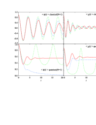
Figure 1: N=1; legend: BVA (solid) , 2PI-1N (dashed), and Hartree (dotted)

Figures 2 and 3 present the time evolution of the one-point functions for the one-filed scenario corresponding to the O(2) and O(4) models, for the CFT and QFT case, respectively. Similar results are shown in Figs. 4 and 5 for the N-copies scenario.

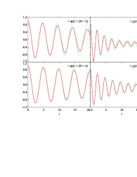
Figure 2: One-field scenario: classical field theory.

Figure 3: One-field scenario: quantum field theory.

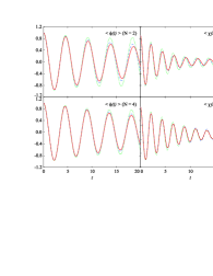
Figure 4: N-copies scenario: classical field theory.

Figure 5: N-copies scenario: quantum field theory.

One striking feature in reviewing these results, is the fact that the NLO corrections are more important in the quantum than in the classical case. The Hartree result represents a poor approximation in QFT, while in CFT it is arguably doing pretty well. This trend is still apparent in the $N=10$ results (not shown). For $N=10$, the differences between 2PI-1/N and BVA for the QFT case have essentially disappeared, but Hartree is still considerably different from NLO in the QFT case.

IV conclusions

We have shown here first calculations of the O(N) model in classical and quantum field theory of the BVA and 2PI-1/N for $N>1$ in 1+1 dimensions. For $N=1$, earlier calculations had shown substantial differences between these two approximations for the quantum field theory case. Our results indicate that these differences diminish for larger values of $N$. The BVA and 2PI-1/N approximations differ through contributions which are proportional to $g^{2}$. Since $g=\lambda/N$, and we chose to keep the coupling constant $\lambda$ fixed, in order to approach the limit of the physically interesting realization of this model (see Refs. Kennedy et al. (1996); Kluger et al. (1995)), this trend was expected, and we have in fact observed it earlier in our previous studies of the quantum mechanical version of this model Mihaila et al. (2001). What is gratifying is the fact that already for $N=4$ the two approximations agree rather well. This gives us hope that our future calculations of the O(4) linear model in 3+1 dimensions will provide reliable predictions, converged with respect to the approximation order. Of course, further numerical evidence will be obtained by carrying out a similar study by carrying out simulations in 2+1 and 3+1 dimensions. An additional study will be pursued in order to provide a better treatment of the three-point vertex, a study which is clearly necessary in order to reduce the differences between the exact and BVA results in 1+1 dimensional classical field theory. It is important to remember that no exact calculations are available for QFT, unlike the CFT case where lattice simulations have been performed. Therefore, the fact that the BVA and 2PI-1/N agree, does not necessarily imply that these approximations also agree with the exact result, and numerical evidence supporting the fact that these further corrections do not affect the results in the O(N) model for $N>1$, is critical to assert the credibility of the results obtained in this approach.