The Peccei–Quinn Field as Curvaton

Abstract:

A simple extension of the minimal supersymmetric standard model which naturally and simultaneously solves the strong CP and $\mu$ problems via a Peccei-Quinn and a continuous R symmetry is considered. This model is supplemented with hybrid inflation and leptogenesis, but without taking the specific details of these scenarios. It is shown that the Peccei-Quinn field can successfully act as a curvaton generating the total curvature perturbation in the universe in accord with the cosmic background explorer measurements. A crucial phenomenon, which assists us to achieve this, is the ‘tachyonic amplification’ of the perturbation acquired by this field during inflation if the field, in its subsequent evolution, happens to be stabilized for a while near a maximum of the potential. In this case, the contribution of the field to the total energy density is also enhanced (‘tachyonic effect’), which helps too. The cold dark matter in the universe consists, in this model, mainly of axions which carry an isocurvature perturbation uncorrelated with the total curvature perturbation. There are also lightest sparticles (neutralinos) which, like the baryons, originate from the inflationary reheating and, thus, acquire an isocurvature perturbation fully correlated with the curvature perturbation. So, the overall isocurvature perturbation has a mixed correlation with the adiabatic one. It is shown that the presently available bound on such an isocurvature perturbation from cosmic microwave background radiation and other data is satisfied. Also, the constraint on the non-Gaussianity of the curvature perturbation obtained from the recent Wilkinson microwave anisotropy probe data is fulfilled thanks to the ‘tachyonic effect’.

1 Introduction

The recent data [1] on the acoustic peaks of the angular power spectrum of the cosmic microwave background radiation (CMBR) strongly favor the idea of inflation, which offers the most elegant solution to the outstanding problems of standard big bang cosmology and exterminates unwanted relics such as monopoles. Moreover, inflation is now generally accepted as the most likely origin of the primordial density perturbations which are needed for explaining the structure formation in the universe [2]. The usual assumption is [2, 3] that these perturbations come solely from the slowly rolling inflaton field. In this case, the observed density perturbations are expected to be purely adiabatic, since fluctuations in the inflaton cannot cause an isocurvature perturbation. Also, significant non-Gaussianity is not encountered [4] in the usual one-field inflationary models, while the non-Gaussianity which is possible [5] in multifield models requires extreme fine-tuning of the initial conditions. However, although adiabatic and Gaussian perturbations are perfectly consistent with the present data, appreciable non-Gaussianity [6] or the presence of a significant isocurvature density perturbation [7, 8] cannot be excluded by observations.

An alternative possibility [9], which has recently attracted attention [10, 11, 12, 13, 14, 15, 16, 17], is that the adiabatic density perturbations originate from the vacuum perturbations during inflation of some light ‘curvaton’ field different from the inflaton. In the curvaton scenario, significant non-Gaussianity may easily appear because the curvaton density is proportional to the square of the curvaton field amplitude. Also, the curvaton density perturbations can lead, after curvaton decay, to isocurvature perturbations in the densities of the various components of the cosmic fluid. In the simplest case, the residual isocurvature perturbations are either fully correlated or fully anti-correlated with the adiabatic density perturbation, with a calculable and generally significant relative magnitude. In the presence of axions, however, the correlation is, in general, mixed. It is important to be noted that the curvaton hypothesis makes [13] the task of constructing viable models of inflation much easier, since it liberates us from the very restrictive requirement that the inflaton is responsible for the curvature perturbations.

The most compelling extension of the standard model (SM) of particle physics is its supersymmetric (SUSY) version, the so-called minimal supersymmetric standard model (MSSM). It is, however, clear that even the MSSM must be part of a larger scheme since it leaves a number of fundamental questions unanswered. For instance, the strong CP and $\mu$ problems cannot be solved in MSSM. Also, it is not easy to generate in MSSM the observed baryon asymmetry of the universe by electroweak sphaleron processes or to realize inflation.

The strong CP problem can be elegantly resolved by including a Peccei-Quinn (PQ) symmetry [18] broken spontaneously at an intermediate mass scale, which can be easily generated within the supergravity (SUGRA) extension of MSSM. The PQ field, which breaks the PQ symmetry, corresponds, in this case, to a flat direction in field space lifted by non-renormalizable interactions. Moreover, the $\mu$ parameter of MSSM can be generated [19] from the PQ scale. A minimal extension of MSSM, which solves the strong CP and $\mu$ problems along these lines, has been constructed in Ref. [20]. A key ingredient was a global $U(1)$ R symmetry obeyed by the superpotential. This model has been further extended [21] to simple SUSY grand unified theory (GUT) models leading to hybrid inflation [22] and yielding successful baryogenesis via a primordial leptogenesis [23, 24] in accord with the data on neutrino masses and mixing. Also, the R symmetry implies exact baryon number conservation, thereby explaining proton stability.

In this paper, we examine whether, in the above models, the PQ field, which possesses an almost flat potential, can also play the role of the curvaton generating the adiabatic curvature perturbations with a possibly significant non-Gaussian component, while accompanied also by an isocurvature density perturbation. An important requirement is that the PQ field is effectively massless during inflation. In view of the quasi-flatness of the potential, one would imagine that this condition could be easily fulfilled by just ensuring that the value of the PQ field during inflation is not too large. However, as it is well-known [25, 26], large SUGRA corrections during inflation can destroy the quasi-flatness of the PQ potential and, thus, invalidate the possibility of using the PQ field as curvaton. Therefore, it is crucial to assume that some mechanism [27] is employed to keep these corrections under control.

After the end of inflation, the inflaton starts performing coherent damped oscillations and eventually decays reheating the universe. We assume that the SUSY breaking corrections to the PQ potential which arise [28] from the finite energy density of the oscillating inflaton field are also relatively small. Under these circumstances, the PQ field remains overdamped and, thus, undergoes a slow evolution for quite some time after the termination of inflation. At later cosmic times, however, it settles into coherent damped harmonic oscillations about zero or the PQ vacua, depending on its value at the end of inflation. Actually, we find that the values of the PQ field at the end of inflation fall into well-defined alternating bands which lead to the trivial (false) vacuum or the PQ vacua in turn. Of course, bands leading to the trivial vacuum must be excluded.

The perturbation acquired by the (light) PQ field during inflation evolves at subsequent times and, when the system settles into damped quadratic oscillations about the PQ vacua, yields a stable perturbation in the energy density of the oscillating field. After the PQ field decays, this perturbation is transferred to the radiation dominated plasma, thereby generating the total curvature perturbation. We find that, if the PQ field, as it evolves, happens to stay near a maximum of the potential for some time, its primordial perturbation from inflation is drastically enhanced and, thus, the resulting energy density perturbation of the oscillating field can be quite sizeable. Also, the contribution of the oscillating field to the total energy density comes out, in this case, larger due to the delay in the onset of the field oscillations caused by the temporary rest of the field near a maximum. Thus, the final curvature perturbation can be adequate to meet the cosmic background explorer (COBE) results [29]. This ‘tachyonic amplification’ of the inflationary perturbation of the PQ field as well as the enhancement of its contribution to the energy density, which occur well after the end of inflation, are crucial for the viability of our scheme.

The cold dark matter (CDM) of the universe, in our case, consists of axions and lightest neutralinos. The latter originate from the late decay of the gravitinos which are generated during the reheating process which follows inflation. In accordance to the curvaton hypothesis, the inflaton and, thus, the radiation which emerges from its decay at reheating possess practically no partial curvature perturbation. Therefore, the baryons, which originate from a primordial leptogenesis taking place at reheating, as well as the neutralinos carry negligible partial curvature perturbation. Then, at curvaton decay, where its curvature perturbation is transferred to the radiation, the baryons and the neutralinos acquire an isocurvature perturbation, which is fully correlated with the total curvature perturbation. The axions, which come into play at the QCD phase transition, also acquire [30] an isocurvature perturbation which is, though, uncorrelated with the total curvature perturbation. So, we finally obtain an isocurvature perturbation of mixed correlation with the curvature perturbation. We apply the most stringent available restriction on such isocurvature perturbations. This restriction results from the set of the CMBR and other data used in Ref. [15].

In our scheme, the curvaton decays somewhat before dominating the energy density of the universe. This can generate appreciable non-Gaussianity in the curvature perturbation. We consider the bound [6] on the possible non-Gaussian component of the curvature perturbation from the recent CMBR data which were obtained by the Wilkinson microwave anisotropy probe (WMAP) satellite. The ‘tachyonic effect’, i.e. the possible rest of the field near a maximum of the potential for a period of time, is essential also for the fulfillment of the non-Gaussianity requirement.

The paper is organized as follows. In section 2, we summarize the minimal extension of MSSM which solves the strong CP and $\mu$ problems via a PQ and a R symmetry. We also indicate the salient features of the simple SUSY GUTs which further extend this model and yield hybrid inflation and successful baryogenesis. In section 3, we outline the evolution of the PQ system during inflation, the subsequent inflaton oscillations and the period after reheating. In section 4, we discuss the conditions under which the PQ field can successfully act as a curvaton. In particular, we consider the constraints on the total curvature and isocurvature perturbation from the COBE results and other data. The requirements from the CDM in the universe are also taken into account. Section 5 is devoted to the detailed numerical analysis of the evolution of the PQ field and its perturbations which originate from inflation. The various requirements of section 4 and the constraints from the non-Gaussianity of the curvature perturbation are numerically studied. Finally, in section 6, we summarize our main conclusions.

2 A simultaneous solution of the strong CP and $\mu$ problems

It is well-known that, in the context of the SUGRA extension of MSSM, appropriate flat directions in field space can generate an intermediate scale

$$M_{I}\sim(m_{3/2}m_{P})^{\frac{1}{2}}\sim 10^{11}-10^{12}\,{\rm GeV},$$ (1)

where $m_{3/2}\sim 1\,{\rm TeV}$ is the SUSY breaking scale and $m_{P}\equiv(8\pi G_{N})^{-1/2}\simeq 2.44\times 10^{18}~{}{\rm GeV}$ is the ‘reduced’ Planck mass with $G_{N}$ being the Newton’s constant. It is then natural to identify the scale $M_{I}$ with the breaking scale $f_{a}$ of a PQ symmetry $U(1)_{\rm PQ}$ [18], which resolves the strong CP problem. Moreover, the $\mu$ parameter of MSSM could be obtained as $\mu\sim f_{a}^{2}/m_{P}\sim m_{3/2}$ [19].

This idea has been elegantly implemented in Ref. [20] in the presence of a non-anomalous R symmetry $U(1)_{R}$. To this end, an extra pair of gauge singlet chiral superfields $N$, $\bar{N}$ with the superpotential couplings

$$\delta W=\frac{\lambda}{2m_{P}}N^{2}\bar{N}^{2}+\frac{\beta}{m_{P}}N^{2}h_{1}h_{2}$$ (2)

was added in MSSM. Here, $h_{1}$ and $h_{2}$ are the two Higgs doublets coupling to the down and up type quarks respectively, and $\lambda$, $\beta$ are dimensionless parameters, which can be made positive by appropriate field redefinitions. The PQ and R charges are

$$PQ:~{}N(-1),~{}\bar{N}(1),~{}h_{1}(1),~{}h_{2}(1),$$

$$R:~{}N(1),~{}\bar{N}(0),~{}h_{1}(0),~{}h_{2}(0)$$ (3)

with the ‘matter’ (quark and lepton) superfields having $PQ=-1/2$, $R=1$. The superpotential has $R=2$. Note that global continuous symmetries such as our PQ and R symmetry can effectively arise [31] from the rich discrete symmetry groups encountered in many compactified string theories (see e.g. Ref. [32]). It should be mentioned in passing that such discrete symmetries can also provide [33] an alternative solution to the $\mu$ problem.

The part of the tree-level scalar potential which is relevant for the PQ symmetry breaking is derived from the superpotential term $\lambda N^{2}\bar{N}^{2}/2m_{P}$ and, after soft SUSY breaking mediated by minimal SUGRA, is given by [20]

$$V_{\rm PQ}=\left(m_{3/2}^{2}+\lambda^{2}\left|\frac{N\bar{N}}{m_{P}}\right|^{2}\right)(|N|^{2}+|\bar{N}|^{2})+\left(Am_{3/2}\lambda\frac{N^{2}\bar{N}^{2}}{2m_{P}}+{\rm h.c.}\right),$$ (4)

where $A$ is the dimensionless coefficient of the soft SUSY breaking term corresponding to the superpotential term $\lambda N^{2}\bar{N}^{2}/2m_{P}$.

The potential $V_{\rm PQ}$ is minimized along the field direction where $N$, $\bar{N}$ have the same magnitude and their phases are arranged so that the last term in the right hand side (RHS) of Eq. (4) becomes negative. The potential then takes the form [20]

$$V_{\rm PQ}=2|N|^{2}m_{3/2}^{2}\left(1-|A|\lambda\frac{|N|^{2}}{2m_{3/2}m_{P}}+\lambda^{2}\frac{|N|^{4}}{m_{3/2}^{2}m_{P}^{2}}\right).$$ (5)

For $|A|>4$, the absolute minimum of the potential is at

$$|\langle N\rangle|=|\langle\bar{N}\rangle|=\left(\frac{|A|+(|A|^{2}-12)^{\frac{1}{2}}}{6\lambda}\right)^{\frac{1}{2}}(m_{3/2}m_{P})^{\frac{1}{2}}\sim(m_{3/2}m_{P})^{\frac{1}{2}}.$$ (6)

The vacuum expectation values (VEVs) of $N$, $\bar{N}$ break spontaneously the symmetry $U(1)_{\rm PQ}\times U(1)_{R}$ down to the discrete ‘matter parity’ symmetry $Z^{\rm mp}_{2}$ under which the ‘matter’ superfields change sign. Substituting these VEVs in Eq. (2), we see that a $\mu$-term with $\mu\sim m_{3/2}$ is generated.

This scheme has been embedded [21] in concrete SUSY GUT models which naturally lead to hybrid inflation [22] followed by a reheating process which satisfies the gravitino constraint [34]. These models also yield successful baryogenesis via a primordial leptogenesis [23] which takes place [24] non-thermally at reheating by the decay of right handed neutrino superfields which emerge from the inflaton decay. The observed baryon asymmetry of the universe can be achieved in accord with the present neutrino oscillation data.

In these models, the PQ and R charges of $N$, $\bar{N}$ and the MSSM superfields are the same as above with the exception of the PQ charge of the left (right) handed quark and lepton superfields which is now $PQ=-1$ ($PQ=0$). This fact implies that the discrete ‘matter parity’ symmetry ($Z^{\rm mp}_{2}$) is now not contained in $U(1)_{\rm PQ}$ and has, thus, to be independently imposed. The VEVs of $N$, $\bar{N}$ break $U(1)_{\rm PQ}\times U(1)_{R}$ completely, while $Z^{\rm mp}_{2}$ again remains exact.

A closer look reveals that the QCD instantons break $U(1)_{\rm PQ}$ explicitly to its $Z_{6}$ subgroup, which is then broken by $\langle N\rangle$, $\langle\bar{N}\rangle$ (as in Refs. [35, 36]). This would lead [37] to a disastrous domain wall production if the PQ transition occurred after inflation. Avoidance of this disaster would then require extending [38] the model so that such spontaneously broken discrete symmetries do not appear. The soft SUSY breaking terms break $U(1)_{R}$ explicitly to its $Z_{2}$ subgroup which, in the presence of $Z^{\rm mp}_{2}$, is equivalent to the $Z_{2}$ under which only $N$ changes sign (compare with Refs. [35, 36]). The breaking of this $Z_{2}$ by $\langle N\rangle$ would also be catastrophic if it took place after inflation. Fortunately, as we will argue in section 3, the $N$, $\bar{N}$ fields emerge with non-zero (homogeneous) values at the end of inflation and, thus, the above discrete symmetries are broken. Also, there is no PQ transition after inflation. Moreover, as we will explain in section 5.1, the system is led to the same minimum of the PQ potential everywhere in space. Consequently, domain walls do not form and there is no need to further complicate the model.

The fact that $N,~{}\bar{N}\neq 0$ after inflation solves yet another problem. It has been shown [35, 36] that the trivial local minimum of $V_{\rm PQ}$ at $N=\bar{N}=0$ is separated from the PQ (absolute) minimum by a sizeable potential barrier. This picture holds [35, 36] at all temperatures below the reheat temperature $T_{\rm reh}\lesssim 10^{9}~{}{\rm GeV}$ [34] even if the one-loop temperature corrections to the potential are included. Thus, after reheating, a PQ transition would have been impossible if the system was in the trivial vacuum. Such a transition could have been even more impossible during inflaton oscillations if the system emerged after inflation being in the trivial vacuum. This is due to the fact that the PQ field typically acquires [28] a positive ${\rm mass}^{2}$ of order $H^{2}$ ($H$ is the Hubble parameter) via its coupling to the inflaton (see section 3).

3 The cosmological evolution of the PQ field

We restrict ourselves on the field direction $\bar{N}^{*}=\pm N\exp{[i(\alpha+\pi)/2]}$ ($\alpha$ is the phase of $A$ in Eq. (4)) along which $V_{\rm PQ}$ is minimized and takes the form in Eq. (5). Rotating $N$ on the real axis by an appropriate R transformation, we can then define the canonically normalized real scalar PQ field $\phi=2N$, which breaks the PQ symmetry and generates the $\mu$-term as discussed in section 2. Eq. (5) then becomes

$$V_{\rm PQ}=\frac{1}{2}m_{3/2}^{2}\phi^{2}\left(1-|A|\lambda\frac{\phi^{2}}{8m_{3/2}m_{P}}+\lambda^{2}\frac{\phi^{4}}{16m_{3/2}^{2}m_{P}^{2}}\right).$$ (7)

For $|A|>4$, this potential has a local minimum at $\phi=0$ and absolute minima at

$$\langle\phi\rangle^{2}\equiv f_{a}^{2}=\frac{2}{3\lambda}\left(|A|+\sqrt{|A|^{2}-12}\right)m_{3/2}m_{P}$$ (8)

with $f_{a}>0$. We can shift the potential $V_{\rm PQ}$ in Eq. (7) by adding to it the constant

$$V_{0}=\frac{1}{108\lambda}\left(|A|+\sqrt{|A|^{2}-12}\right)\left[|A|\left(|A|+\sqrt{|A|^{2}-12}\right)-24\right]m_{3/2}^{3}m_{P},$$ (9)

so that it vanishes at its absolute minima.

In order to be able to study the cosmological evolution of $\phi$, we should first include the SUSY breaking effects which arise [25, 26, 28] from the fact that the energy density in the early universe is finite. During inflation and the subsequent inflaton oscillations, SUSY breaking is transmitted to the PQ system via its coupling to the inflaton given by the SUGRA scalar potential. The scale of the resulting SUSY breaking terms is set by the Hubble parameter $H$ and, thus, these terms dominate over the terms from hidden sector SUSY breaking as long as $H\gtrsim m_{3/2}$.

We should point out that, during the era of inflaton oscillations, the PQ potential acquires temperature corrections too. They originate from the ‘new’ radiation [39] which emerges from the decaying inflaton and has temperature $T\sim(Hm_{P}T_{\rm reh}^{2})^{1/4}$. Their scale is set by the thermally induced mass for the PQ field. A typical contribution ($\sim\beta NT/m_{P}$) to this mass is given by the second term in the RHS of Eq. (2) with the Higgsino lines connected to a loop via a mass insertion. However, this contribution exists only under the condition that the effective Higgsino mass ($\sim\beta N^{2}/m_{P}$) does not exceed $T$. For our input numbers (see section 5) and almost until the end of the period when $H\gtrsim m_{3/2}$, we can show that, whenever this condition is satisfied, we also have $\beta NT/m_{P}\lesssim H$, which means that the temperature corrections are overshadowed by the SUGRA ones. At later times, $N$ becomes anyway adequately small and, thus, the thermally induced mass for the PQ field comes out much smaller than $H$. We, thus, conclude that the temperature corrections can be neglected throughout the era of inflaton oscillations.

After reheating, where $H\ll m_{3/2}$ as a consequence of the gravitino constraint ($T_{\rm reh}\lesssim 10^{9}~{}{\rm GeV}$) [34], the (one-loop) temperature corrections to the PQ potential could be the main source of SUSY breaking. However, as shown in Refs. [35, 36], these corrections are less important than the ones from the hidden sector. This is understood from the fact that $N$, $\bar{N}$ possess only non-renormalizable interactions which are suppressed by $m_{P}$ and carry relatively small dimensionless coupling constants.

In our case, the SUSY breaking corrections to the PQ potential during the inflationary and oscillatory phases can generally be [28] of two types:

$$H^{2}m_{P}^{2}f(\phi^{2}/m_{P}^{2}),$$ (10)

$$Hm_{P}^{3}g(\phi^{4}/m_{P}^{4}),$$ (11)

where $f$, $g$ are some functions depending on the model, the Kähler potential and the phase. To the leading approximation, the correction in Eq. (10) yields a mass term $\delta m_{\phi}^{2}\phi^{2}/2$ for the curvaton $\phi$. For a general Kähler potential, $\delta m_{\phi}^{2}\sim H^{2}$ with either sign possible. However, for specific (no-scale like) forms of the Kähler potential, this induced ${\rm mass}^{2}$ might be (partially) cancelled [27]. For simplicity, we will approximate the correction in Eq. (10) by the mass term. We will also assume that $\delta m_{\phi}^{2}$ is positive and somewhat suppressed. We, thus, write

$$\delta m_{\phi}=\gamma H,$$ (12)

where $\gamma\sim 0.1$ and can have different values during inflation and field oscillations. The correction in Eq. (11) is of the $A$ term type with $A\sim H$ and, although it is generally present, we will not take it into account in order to simplify the analysis. We will, thus, consider the following full scalar potential

$$V(\phi)=V_{\rm PQ}+\frac{1}{2}\gamma^{2}H^{2}\phi^{2}+V_{0}.$$ (13)

The evolution of the field $\phi$ is governed by the classical equation of motion

$$\ddot{\phi}+3H\dot{\phi}+V^{\prime}(\phi)=0,$$ (14)

where overdots and primes denote derivation with respect to the cosmic time $t$ and the field $\phi$ respectively. Here, the damping term, proportional to the Hubble parameter, arises from the expansion of the universe. For large values of $\phi$, the potential $V_{\rm PQ}$ in Eq. (7) is dominated by the non-renormalizable $\phi^{6}$-term. Moreover, for $H\gg m_{3/2}$, the induced mass in Eq. (12) can also be important. Hence, if $\phi$ happens to be large during some stage of inflation, we can write

$$V(\phi)\simeq\frac{1}{2}\gamma^{2}H_{\rm infl}^{2}\phi^{2}+\lambda^{2}\frac{\phi^{6}}{32m_{P}^{2}}+V_{0},$$ (15)

where $H_{\rm infl}$ is the inflationary Hubble parameter. It is natural to assume that, at the onset of inflation, $V(\phi)\lesssim V_{\rm infl}$, where $V_{\rm infl}$ is the (almost) constant vacuum energy density which is provided by the inflaton and drives the exponential expansion of the universe. Thus, $\phi$ may initially be quite large. For such values of $\phi$, $V^{\prime\prime}$ is dominated by the $\phi^{6}$-term in the potential in Eq. (15) and the system is initially underdamped ($V^{\prime\prime}\gg H_{\rm infl}^{2}$). Consequently, $\phi$ decreases rapidly and $V^{\prime\prime}$ quickly falls below $H_{\rm infl}^{2}$ with the system entering into a regime of slow-roll evolution. Soon after this, the induced mass term in Eq. (15) becomes dominant.

The classical equation of motion holds until the quantum perturbations of $\phi$ generated by inflation, $\delta\phi=H_{\rm infl}/2\pi$, overshadow its classical kinetic energy density $\rho_{\rm kin}=\dot{\phi}^{2}/2$. These perturbations contribute a ‘quantum’ kinetic energy density of order $(\delta\phi/\delta t)^{2}/2$, where $\delta t\sim H_{\rm infl}^{-1}$. Therefore, the slow-roll regime will end when $\rho_{\rm kin}\sim H_{\rm infl}^{4}/8\pi^{2}$. From the slow-roll equation $\dot{\phi}\simeq-V^{\prime}(\phi)/3H_{\rm infl}$ derived from Eq. (14), we then find that this happens [40] at $\phi\sim\phi_{Q}$, where $\phi_{Q}$ is given by

$$V^{\prime}(\phi_{Q})\simeq\gamma^{2}H_{\rm infl}^{2}\phi_{Q}\sim\frac{3H_{\rm infl}^{3}}{2\pi}.$$ (16)

The subsequent evolution of $\phi$ is controlled by its quantum perturbations which ‘kick’ it around to perform a ‘random walk’. This results to a ‘quantum drift’ of the average value of $\phi$ towards smaller values (since it cannot be pushed over $\phi_{Q}$) in the sense that the field’s distribution spreads towards the origin, which is finally engulfed inside an evenly spread stationary distribution whose width is $\phi_{Q}$. Thus, the value $\phi_{f}$ of $\phi$ at the end of inflation, taken positive without loss of generality, can be smaller than $\phi_{Q}$ if sufficiently many e-foldings take place after $\phi_{Q}$, but it is typically $\sim\phi_{Q}$. At the termination of inflation, the quantum perturbations of $\phi$ cease and the field emerges with vanishing kinetic energy.

Of course, depending on the total number of e-foldings during inflation and the value of $\phi$ at the onset of inflation, the inflationary phase may be terminated while $\phi$ is still in the slow-roll regime. In this case, we have $\phi_{f}\gtrsim\phi_{Q}$ and $\dot{\phi}_{f}\simeq-\gamma^{2}H_{\rm infl}\phi_{f}/3-\lambda^{2}\phi_{f}^{5}/16m_{P}^{2}H_{\rm infl}$. For the values used here, the corresponding kinetic energy density is much smaller than the potential energy density and can be neglected. In summary, the field $\phi$ can practically have any value $\phi_{f}$ at the end of inflation. However, if $\phi_{f}$ is smaller than a certain large limit (depending on $\lambda$) so that $\phi$ is slowly rolling or in the ‘quantum’ regime as inflation ends, the field $\phi$ emerges with vanishing velocity. This sets the initial conditions for the subsequent evolution of the PQ field.

After inflation, the universe enters into a matter dominated era where the energy density is provided by the coherent oscillations of the inflaton. The potential $V(\phi)$ is then given by Eq. (13) with $H=2/3t$. If $\phi$ is slowly rolling at the end of inflation, the friction term in Eq. (14) remains important at subsequent times too and the evolution of $\phi$ is slow for quite some time. As the cosmic time increases, the Hubble parameter decreases and, thus, at some point, the induced mass in Eq. (12) becomes $\lesssim m_{3/2}$. After this point, the soft terms arising from SUSY breaking by the energy density of the oscillating inflaton are smaller than the ones from hidden sector SUSY breaking. Therefore, the potential can be approximated as

$$V(\phi)\simeq V_{\rm PQ}+V_{0},$$ (17)

with $V_{\rm PQ}$ given in Eq. (7), and has a local minimum at the origin with $V=V_{0}$, absolute minima at $\phi=\pm f_{a}$ with $V=0$ and local maxima at $\phi=\pm\phi_{\rm max}$, where

$$\phi^{2}_{\rm max}=\frac{2}{3\lambda}\left(|A|-\sqrt{|A|^{2}-12}\right)m_{3/2}m_{P}$$ (18)

with

$$V_{\rm max}=\frac{1}{27\lambda}(|A|^{2}-12)^{\frac{3}{2}}m_{3/2}^{3}m_{P}$$ (19)

and $\phi_{\rm max}>0$. Soon after this, $H$ becomes $\lesssim m_{3/2}$ and the system enters into a phase of damped oscillations about either the trivial minimum at $\phi=0$ or one of the PQ minima at $\phi=\pm f_{a}$, depending on the value of $\phi$ at $t\sim m_{3/2}^{-1}$.

After reheating, $H=1/2t\ll m_{3/2}$. So, the system remains underdamped and $V(\phi)$ is still given by Eq. (17). (Recall that the temperature corrections to the potential are not important.) The field $\phi$ keeps performing damped oscillations about one of the minima until it finally decays. These minima are separated by sizeable potential barriers and, thus, a transition from the trivial to a PQ minimum cannot occur. So, if the field was driven to the trivial minimum, it would be trapped there forever. The PQ symmetry would then remain unbroken and the strong CP problem would not be solved, while the universe would experience an unacceptably large effective cosmological constant.

4 The PQ field as curvaton

In accordance with the recently investigated [10, 11, 12, 13, 14, 15, 16, 17] curvaton scenario, the curvature perturbations may originate from the quantum perturbations during inflation not of the inflaton but rather of another light field which has been called curvaton. In this section, we will address the question whether our PQ field $\phi$ can successfully act as a curvaton. To this end, we must first consider the following two requirements:

1. As already mentioned, the energy density of the universe during inflation must be dominated by $V_{\rm infl}$, the vacuum energy density provided by the inflaton. (Here, $V_{\rm infl}$ is assumed to be essentially constant.) Therefore, the value of the PQ field during and at the end of inflation should be bounded above by the requirement $V(\phi)\lesssim V_{\rm infl}$. For definiteness, we take here the standard SUSY hybrid inflationary scheme [26, 41] (for a recent review see e.g. Ref. [36]). The inflationary scale is then given by

   $$V^{\frac{1}{4}}_{\rm infl}=\kappa^{\frac{1}{2}}M,$$ (20)

   where $\kappa$ and $M$ are the dimensionless parameter and the mass scale of the standard superpotential for hybrid inflation respectively. For simplicity, we identify $M$ with the SUSY GUT scale $M_{\rm GUT}\simeq 2.86\times 10^{16}~{}{\rm GeV}$.

2. A much more stringent constraint is obtained from the requirement that the field $\phi$ is effectively massless during (at least) the last $50-60$ inflationary e-foldings so that it receives a superhorizon spectrum of perturbations [42]

   $$\delta\phi=\frac{H_{\rm infl}}{2\pi}$$ (21)

   from inflation. This requirement means that $V^{\prime\prime}(\phi)\lesssim H_{\rm infl}^{2}$, which guarantees also that $\phi$ is of negligible time derivative at the end of inflation.

The detailed evolution of the inflationary perturbations of $\phi$ after inflation will be considered in the next section. For the moment, we will only discuss how these perturbations can generate (or affect) the total curvature perturbation

$$\zeta=-H\frac{\delta\rho}{\dot{\rho}}=\frac{\delta\rho}{3(\rho+p)},$$ (22)

where $\rho$ and $p$ are the total energy density and pressure in the universe respectively. As we approach the time at which the curvaton decays, the universe is normally dominated by radiation and the oscillating curvaton $\phi$. In this case, we can write

$$\zeta=(1-f)\zeta_{r}+f\zeta_{\phi},$$ (23)

where $\zeta_{r}=\delta\rho_{r}/4\rho_{r}$,  $\zeta_{\phi}=\delta\rho_{\phi}/3\rho_{\phi}$ and

$$f=\frac{3\rho_{\phi}}{3\rho_{\phi}+4\rho_{r}}$$ (24)

with $\rho_{r}$ and $\rho_{\phi}$ being the radiation and $\phi$ energy densities respectively. Here, we assumed that the amplitude of the oscillating $\phi$ has been adequately reduced so that the potential can be approximately considered as quadratic. The oscillating curvaton then resembles pressureless matter and $\delta\rho_{\phi}/\rho_{\phi}=2\,\delta\phi_{0}/\phi_{0}$, where $\phi_{0}$ is the amplitude of the oscillations and $\delta\phi_{0}$ the perturbation in this amplitude originating from $\delta\phi$ in Eq. (21). According to the curvaton hypothesis, the inflaton contribution to the density perturbation is insignificant. Consequently, the radiation emerging from the inflaton decay has $\zeta_{r}\simeq 0$. After the curvaton decay, we obtain the final curvature perturbation which, in the instantaneous decay approximation, is given by

$$\zeta\simeq f_{\rm dec}\zeta_{\phi},$$ (25)

where $f_{\rm dec}$ is the value of $f$ at the decay of the curvaton. The COBE measurements require [29] that $\zeta\simeq 5\times 10^{-5}$.

If the curvaton field decays well before dominating the energy density of the universe (i.e. $f_{\rm dec}\ll 1$), which is the case here, the total curvature perturbation can acquire [11] a significant non-Gaussian component. The reason is that the curvature perturbation is proportional to the perturbation of the curvaton energy density (see Eq. (25)), which depends on the square of $\phi$. This is interesting since the recent CMBR data from the WMAP satellite leave [6] considerable room for non-Gaussianity in the curvature perturbations. We will come back to this point in the next section where a detailed numerical analysis of the model will be presented.

As mentioned in section 3, after the end of inflation, the inflaton performs damped oscillations and eventually decays into light particles reheating the universe. The reheat temperature $T_{\rm reh}$ is related [3] to the inflaton decay width $\Gamma_{\rm infl}$ by

$$T_{\rm reh}=\left(\frac{45}{2\pi^{2}g_{*}}\right)^{\frac{1}{4}}(\Gamma_{\rm infl}m_{P})^{\frac{1}{2}},$$ (26)

where $g_{*}$ is the effective number of degrees of freedom. After reheating, gravitinos ($\tilde{g}$) are thermally produced besides other particles. They only decay, though, well after the big bang nucleosynthesis (BBN) since they have very weak couplings. The decay channels normally include the one to a photon and a photino ($\tilde{g}\rightarrow\gamma+\tilde{\gamma}$) with the emerging high energy photons causing the dissociation of the light elements and, thus, destroying the successful predictions of BBN. This yields [34] the strongest possible upper bound on the reheat temperature, which is $T_{\rm reh}\lesssim 10^{9}~{}{\rm GeV}$ if the branching ratio to photons equals unity and the gravitino mass $m_{3/2}$ is in the range of several hundreds of GeV. However, the upper bound can be considerably relaxed [34, 43] if this branching ratio is less than unity.

Each decaying gravitino yields one sparticle subsequently turning into the lightest sparticle (LSP), which is stable. This is due to the presence of ‘matter parity’ in our model. Moreover, no pair annihilation of the resulting LSPs is possible since the universe is already quite cold. Consequently, these LSPs survive until the present time contributing to the relic abundance of CDM in the universe. We will assume, as it is customary, that the LSP is the lightest neutralino ($\tilde{\chi}$). We will also make the simplifying assumption that the relic abundance of the thermally produced LSPs is negligible, which holds in many cases. So, the relic abundance, $\Omega_{\rm LSP}h^{2}$, of the LSPs comes solely from the decaying gravitinos and can be estimated following Ref. [43]. Here, $\Omega_{\rm LSP}=\rho_{\rm LSP}/\rho_{c}$ with $\rho_{\rm LSP}$ ($\rho_{c}$) being the LSP (critical) energy density and $h\simeq 0.71$ is the present Hubble parameter in units of $100~{}\rm{km}~{}\rm{sec}^{-1}~{}\rm{Mpc}^{-1}$.

Our model contains axions which can also contribute to the CDM of the universe. Their relic abundance, $\Omega_{a}h^{2}$, can be calculated by applying the formulae of Ref. [44] ($\Omega_{a}=\rho_{a}/\rho_{c}$ with $\rho_{a}$ being the axion energy density). For simplicity, we take the QCD scale $\Lambda=200~{}{\rm GeV}$ and ignore the uncertainties in these formulae. Also, the anharmonic effects are negligible in our case and the possibility of entropy production after the QCD transition is not considered. The total CDM abundance is the sum of the relic abundance of the LSPs from the gravitino decays and the relic axion abundance ($\Omega_{\rm CDM}=\rho_{\rm CDM}/\rho_{c}$ with $\rho_{\rm CDM}$ being the CDM energy density):

$$\Omega_{\rm CDM}h^{2}\simeq 0.0074\left(\frac{m_{\rm LSP}}{200~{}{\rm GeV}}\right)\left(\frac{T_{\rm reh}}{10^{9}~{}{\rm GeV}}\right)+\theta^{2}\left(\frac{f_{a}}{10^{12}~{}{\rm GeV}}\right)^{1.175},$$ (27)

where $m_{\rm LSP}$ is the LSP mass and $\theta$ the so-called initial misalignment angle, i.e. the phase of the complex PQ field at the end of inflation. The angle $\theta$ lies in the interval $[-\pi/{\cal N},\pi/{\cal N}]$, where ${\cal N}$ is the absolute value of the sum of the PQ charges of all fermionic color (anti)triplets. This same ${\cal N}$ determines the $Z_{\cal N}$ subgroup of $U(1)_{\rm PQ}$ which remains unbroken by instantons. As mentioned in section 2, in our (and the simplest) model, ${\cal N}=6$. All $\theta$’s in the above interval are equally probable.

It is well-known that all the effectively massless (non conformally invariant) fields acquire a superhorizon spectrum of perturbations during inflation. So, such perturbations are generated in the axion field too. When the axion mass comes into play at the QCD phase transition, these perturbations become isocurvature axion density perturbations. The late universe consists, in our case, of axions ($a$), baryons ($B$) and neutralinos ($\tilde{\chi}$) as matter, and photons ($\gamma$) and (massless) neutrinos ($\nu$) as radiation. In order to extract the restrictions on our model which come from isocurvature perturbations, we employ the analysis of Ref. [8]. We, thus, consider the comoving curvature perturbation $\mathcal{R}_{\rm rad}$ and the isocurvature perturbation $\mathcal{S}_{\rm rad}$ determining the large scale CMBR temperature perturbation. They are given by

$$\mathcal{R}_{\rm rad} = -\zeta,$$ (28)

$$\mathcal{S}_{\rm rad}\hat{a} = \sum_{i=a,B,\tilde{\chi}}\frac{\Omega_{i}}{\Omega_{m}}S_{i}\hat{a}_{i},$$ (29)

where $S_{i}=\delta n_{i}/n_{i}-3\,\delta T/T$ ($i=a,~{}B,~{}\tilde{\chi}$) is the isocurvature perturbation in the $i$th species, $\hat{a}$, $\hat{a}_{i}$ are appropriate Gaussian random variables, $\Omega_{i}=\rho_{i}/\rho_{c}$ and $\Omega_{m}=\rho_{m}/\rho_{c}$ with $\rho_{i}$ and $n_{i}$ being the energy and number densities of the $i$th species and $\rho_{m}=\rho_{a}+\rho_{B}+\rho_{\tilde{\chi}}$ being the matter energy density.

The neutralinos appear as decay products of the gravitinos which were generated at reheating. They, thus, inherit the same curvature perturbation, which coincides with that of radiation emerging from the inflaton decay. However, $\zeta_{r}\simeq 0$ by the curvaton hypothesis and, consequently, $\zeta_{\tilde{\chi}}=\delta\rho_{\tilde{\chi}}/3\rho_{\tilde{\chi}}$ also vanishes. After the curvaton decay, the neutralino isocurvature perturbation $S_{\tilde{\chi}}\equiv 3(\zeta_{\tilde{\chi}}-\zeta_{\gamma})\simeq-3\zeta$. Here, we assumed that the neutrino isocurvature perturbation is negligible and, thus, $\zeta_{\gamma}=\delta\rho_{\gamma}/4\rho_{\gamma}\simeq\zeta$ ($\rho_{\gamma}$ is the photon energy density). Baryons can be produced via a primordial leptogenesis [23] which can occur [24] at reheating. The inflaton decays into right handed neutrino superfields which, subsequently, decay into Higgs and lepton superfields generating a net lepton number. As a consequence, $\zeta_{B}\simeq 0$ too and again $S_{B}\equiv 3(\zeta_{B}-\zeta_{\gamma})\simeq-3\zeta$. We see that the baryons and the neutralinos carry an isocurvature perturbation which is fully correlated with the isentropic perturbation in the notation of Ref. [8].

The axions are produced at the QCD phase transition which takes place comfortably after the curvaton decay. At this transition, the axion mass $m_{a}$ is generated and the axion field starts oscillating. For the amplitudes $a$ encountered here, the anharmonic effects [44] are negligible and, thus, the axion energy density is given by $\rho_{a}=m_{a}^{2}a^{2}/2$. The isocurvature perturbation which is generated is then $S_{a}=\delta n_{a}/n_{a}=\delta\rho_{a}/\rho_{a}=2\,\delta a/a$. The perturbation $\delta a$ in the amplitude of the axion field comes from inflation and can be estimated [45] as follows. Suppose that $\phi_{*}$ is the value of $\phi$ when our present horizon scale crosses outside the inflationary horizon (i.e. $\sim 50-60$ e-foldings before the end of inflation) and $\theta$ is the initial misalignment angle, i.e. the phase of the complex PQ field during (and at the end of) inflation. This angle corresponds to the canonically normalized real scalar field $\theta\phi_{*}$ which acquires a perturbation $H_{\rm infl}/2\pi$ from inflation and, thus, $\delta\theta=H_{\rm infl}/2\pi\phi_{*}$. The initial amplitude of axion oscillations $a=\theta f_{a}$ then acquires a perturbation $\delta a=H_{\rm infl}f_{a}/2\pi\phi_{*}$. We see that the axion isocurvature perturbation is $S_{a}=H_{\rm infl}/\pi\theta\phi_{*}$. This perturbation is completely uncorrelated with the curvature perturbation.

Replacing $S_{a}$, $S_{B}$ and $S_{\tilde{\chi}}$ in Eq. (29), we obtain

$$\mathcal{S}_{\rm rad}\hat{a}=\left(\frac{H_{\rm infl}}{\pi\theta\phi_{*}}\frac{\Omega_{a}}{\Omega_{m}}\hat{a}_{a}-3\zeta\frac{\Omega_{B}+\Omega_{\tilde{\chi}}}{\Omega_{m}}\hat{a}_{B}\right),$$ (30)

which consists of an uncorrelated and a fully correlated part. Here, the Gaussian random variables $\hat{a}_{a}$, $\hat{a}_{B}=\hat{a}_{\tilde{\chi}}$ are independent. The dimensionless cross correlation parameter is given by [8]

$$\cos\Delta=\frac{3}{B}\left(1-\frac{\Omega_{a}h^{2}}{\Omega_{m}h^{2}}\right),$$ (31)

where

$$B=\left[\left(\frac{H_{\rm infl}}{\pi\theta\phi_{*}\zeta}\right)^{2}\left(\frac{\Omega_{a}h^{2}}{\Omega_{m}h^{2}}\right)^{2}+9\left(1-\frac{\Omega_{a}h^{2}}{\Omega_{m}h^{2}}\right)^{2}\right]^{\frac{1}{2}}.$$ (32)

is the entropy-to-adiabatic ratio. In Ref. [8], a bound on this ratio has been derived from the pre-WMAP CMBR data and was depicted in Fig. 2 of this reference versus $\cos\Delta$ with the other parameters marginalized. We take an improved version [46] of this figure, which can be derived from the extended set of pre-WMAP data used in Ref. [15], and extract from it the $95\%$ confidence level (c.l.) bound on $B$ for each value of $\cos\Delta$. At present, this is the most stringent available bound on isocurvature perturbations of mixed correlation with the curvature perturbation.

5 Numerical analysis and results

5.1 The band structure

We are now ready to study numerically the evolution of the PQ field after inflation. To this end, we perform the change of variable

$$t=H_{\rm infl}^{-1}e^{\tau}$$ (33)

in Eq. (14), which then becomes

$$\frac{d^{2}\phi}{d\tau^{2}}+\left(3e^{\tau}\frac{H}{H_{\rm infl}}-1\right)\frac{d\phi}{d\tau}+\frac{e^{2\tau}}{H_{\rm infl}^{2}}V^{\prime}(\phi)=0.$$ (34)

Inflation ends at $t=t_{f}\simeq(2/3)H_{\rm infl}^{-1}$. So, we impose the initial conditions $\phi=\phi_{f}>0$ and $d\phi/d\tau=0$ at $\tau=\ln(2/3)$. Although, as explained in section 3, the field $\phi$ exits inflation with negligible velocity only if $\phi_{f}$ is not too large, we will apply these initial conditions uniformly for all values of $\phi_{f}$ in order to obtain an overall picture of the possible behavior patterns of the system. We will, of course, use only the relevant $\phi_{f}$’s to draw physical conclusions. As we already mentioned, these $\phi_{f}$’s practically coincide with the $\phi_{f}$’s for which the PQ field is effectively massless during inflation so that it acquires a superhorizon spectrum of perturbations.

The Hubble parameter during inflation $H_{\rm infl}$ is given by the Friedmann equation

$$H_{\rm infl}^{2}=\frac{V_{\rm infl}}{3m_{P}^{2}}=\frac{\kappa^{2}M_{\rm GUT}^{4}}{3m_{P}^{2}},$$ (35)

where the almost constant energy density $V_{\rm infl}$ driving inflation is taken from Eq. (20) which holds in the case of standard SUSY hybrid inflation. We do not commit ourselves to any details of this inflationary scheme. We also leave out the possible restrictions from the specific reheating and leptogenesis processes in the SUSY GUT models of Ref. [21]. We just use, for our analysis, the inflationary scale derived from Eq. (20) as a working example. For definiteness, we further take $\kappa=10^{-3}$, which gives $V_{\rm infl}^{1/4}\simeq 9.04\times 10^{14}~{}{\rm GeV}$ and $H_{\rm infl}\simeq 1.97\times 10^{11}~{}{\rm GeV}$. It should be noted that this inflationary scale is consistent with the curvaton hypothesis which requires [13] that $V^{1/4}_{\rm infl}\lesssim 3\times 10^{15}~{}{\rm GeV}$. Indeed, if this condition holds, the curvature perturbation from the inflaton can be made negligible.

The scalar potential $V(\phi)$ is taken from Eq. (13), where we put $m_{3/2}=300~{}{\rm GeV}$, $|A|=5$ and $\gamma=0.1$. The parameter $\lambda$ is taken to range between $10^{-4}$ and $10^{-3}$. Fixing the reheat temperature $T_{\rm reh}$ to the value $10^{9}~{}{\rm GeV}$ [34] and taking $g_{*}=228.75$ which corresponds to the MSSM spectrum, Eq. (26) yields the inflaton decay time $t_{\rm reh}=\Gamma_{\rm infl}^{-1}\simeq 2.44\times 10^{-1}~{}{\rm GeV}^{-1}$. For $t_{f}\leq t\leq t_{\rm reh}$, the universe is dominated by the oscillating inflaton and $H=2/3t$. The expression in parentheses in Eq. (34) is then equal to unity. For $t\geq t_{\rm reh}$, however, radiation dominates and $H=1/2(t-t_{\rm reh}/4)$. Here, we subtracted $t_{\rm reh}/4$ from $t$ in order to achieve continuity at $t=t_{\rm reh}$. For $t\gg t_{\rm reh}$, the expression in parentheses in Eq. (34) equals $1/2$.

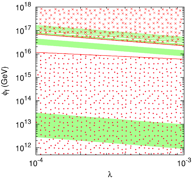
Figure 1: The band structure in the $\lambda-\phi_{f}$ plane. If $\phi_{f}$ lies in a green (white) band, the system is led into a PQ (the false) vacuum. The red crossed area is excluded by requiring that the PQ field is light during the relevant part of inflation, while the red dotted area is excluded by the bound on the isocurvature perturbation from the CMBR data.

Using the above described initial conditions and numerical inputs, we now solve Eq. (34) numerically. For each value of $\phi_{f}$ and any given $\lambda$ in the range $10^{-4}-10^{-3}$, we follow the evolution of the system and identify the minimum of $V_{\rm PQ}$ about which the PQ field is finally set in coherent damped oscillations. We find that a well-defined band structure emerges in the $\lambda-\phi_{f}$ plane. This structure is depicted in Fig. 1 with alternating white and green bands. We number the successive bands starting from zero which is given to the lowest lying (white) band. So, the white bands correspond to even integers, while the green ones to odd integers. We only show the first 18 bands since after this the bands become too dense in the figure to be clearly distinguishable. If the initial value of the field $\phi_{f}$ belongs to a white band, the system is finally led into the false vacuum at $\phi=0$. So, such $\phi_{f}$’s are excluded. However, if $\phi_{f}$ lies in a green band, the system ends up in one of the PQ vacua. The boundaries of the bands in Fig. 1, which is a $\log-\log$ plot, are parallel straight lines with an inclination equal to $-1/2$. This is easily understood by observing that, if $\phi$ is rescaled by absorbing a $\lambda^{1/2}$ factor, Eq. (34) becomes $\lambda$-independent.

As indicated in section 4, the PQ field must be light during the last $50-60$ e-foldings (i.e. $V^{\prime\prime}(\phi)\lesssim H_{\rm infl}^{2}$) so that it acquires perturbations from inflation which enable it to act as curvaton. In particular, at the end of inflation, we must require that $V^{\prime\prime}(\phi_{f})\lesssim H_{\rm infl}^{2}$, which excludes the red crossed area in Fig. 1. The boundary of this area is again a straight line with an inclination equal to $-1/2$ and turns out to be very close to the lower boundary of the 5th (green) band. So, out of all the odd (green) bands, only the 1rst and 3rd are consistent with the above requirement, while all the higher green bands are excluded. We find that, in the non-excluded area, $\phi$ remains practically constant in the last $50-60$ e-foldings and, thus, the condition $V^{\prime\prime}(\phi)\lesssim H_{\rm infl}^{2}$ is valid throughout this period. It is obvious that, in this same area, the field velocity at the end of inflation is negligible. Finally, we should note that, in this allowed area, the condition $V(\phi)\lesssim V_{\rm infl}$, which, as explained in section 4, must hold during inflation, is automatically satisfied provided that the total number of inflationary e-foldings is not huge.

It should be emphasized that the non-vanishing of $N$, $\bar{N}$ after inflation alone cannot guarantee the avoidance of disastrous domain walls. It is crucial to further ensure that the system finally relaxes in the same minimum over all space. This is readily fulfilled in our case since the perturbation $\delta\phi=H_{\rm infl}/2\pi\simeq 3.14\times 10^{10}~{}{\rm GeV}$, which is acquired by the PQ field during inflation, is much smaller than the width of the bands. Therefore, right after inflation, the field is found to lie within the same band everywhere in space. It is then led into the same minimum over all space and no catastrophic domain wall production occurs. The opposite situation has been encountered in Ref. [47], where the inflationary perturbation of the field could become comparable to or even larger than the width of the bands. As a consequence, topological defects could be generated.

We will now consider the bound on the entropy-to-adiabatic ratio $B$ in Eq. (32) which has been derived in Ref. [8] from the pre-WMAP CMBR data. We take the baryon abundance $\Omega_{B}h^{2}=0.02$, which is [48] its central value from BBN. The CDM abundance, $\Omega_{\rm CDM}h^{2}$, is taken equal to its central value $0.12$ from DASI [49]. Thus, the total matter abundance is $\Omega_{m}h^{2}=0.14$. The axion abundance $\Omega_{a}h^{2}$ (second term in the RHS of Eq. (27)) can then be calculated from Eq. (27), where we put $m_{\rm LSP}=200~{}{\rm GeV}$. We find that the axions constitute about $94\%$ of the CDM. From this, we find the initial misalignment angle $\theta$ for each $\lambda$. The curvature perturbation $\zeta$ is taken equal to $5\times 10^{-5}$ from COBE [29]. As we saw, $\phi$ remains practically constant in the last $50-60$ e-foldings provided that we are outside the red crossed area of Fig. 1. Thus, in the relevant area, the value $\phi_{*}$ of $\phi$ when our present horizon crossed outside the inflationary horizon can be identified with $\phi_{f}$. We apply an improved version [46] of the $95\%$ c.l. bound on $B$ for each value of the cross correlation parameter $\cos\Delta$ in Eq. (31). This yields a lower bound on $\phi_{f}$ for each $\lambda$ excluding the red dotted area in Fig. 1. The boundary of this area is a straight line with an inclination equal to $-1.175/4\simeq-0.294$ as one can easily deduce from Eqs. (8), (27), (31) and (32).

We see that the bound from the isocurvature perturbation excludes the 1rst (green) band and, thus, only the 3rd (green) band survives. Note, though, that this bound actually pushes $\phi_{*}$ and not $\phi_{f}$ to large values. Moreover, in the last $50-60$ e-foldings, such a large $\phi_{*}$ could be reduced to a $\phi_{f}$ lying in the 1rst band if $\phi$ was rolling fast. However, this would require a large SUGRA induced curvaton mass during inflation, which is incompatible with the curvaton hypothesis. Finally, we should stress that the fact that the CDM consists mainly of axions carrying an isocurvature perturbation which is uncorrelated with the curvature perturbation is of crucial importance for the viability of the model. Indeed, it leads to a cross correlation parameter $\cos\Delta$ which is somewhat smaller than unity and, thus, the upper bound on the entropy-to-adiabatic ratio $B$ is considerably relaxed. Actually, in our case, this bound takes its maximal value ($\simeq 0.95$) which is achieved in the range $0.55\lesssim\cos\Delta\lesssim 0.75$.

5.2 The evolution patterns of the PQ field

Let us now describe in some detail the time dependence of the full curvaton potential $V(\phi)$ in Eq. (13) and the evolution of the PQ field $\phi$ after the end of inflation in accordance with our numerical findings. For definiteness, we fix $\lambda=10^{-4}$. To obtain the picture for other values of $\lambda$, we just have to rescale $V$ as $\lambda^{-1}$ and $\phi$ as $\lambda^{-1/2}$. In Fig. 2, we present a three dimensional plot of $V(\phi)$ as a function of $\phi$ and the cosmic time $t$. We see that, initially and for small $\phi$’s, the induced mass in Eq. (12) dominates over the soft SUSY breaking terms in Eq. (4) and, thus, $V(\phi)$ has just one minimum at zero. At later times, the induced mass becomes comparable to the soft terms and $V(\phi)$ develops a pair of symmetric local minima separated from the trivial minimum (at zero) by a pair of symmetric local maxima. The height of the local minima is gradually reduced and, at some point, they become absolute minima. Finally, when $t\gtrsim 2\gamma/3m_{3/2}\simeq 2.22\times 10^{-4}~{}{\rm GeV}^{-1}$, the induced mass becomes subdominant and, thus, $V(\phi)$ can be approximated as in Eq. (17). The above (non-trivial) minima then approach the PQ vacua at $\phi=\pm f_{a}\simeq\pm 6.48\times 10^{12}~{}{\rm GeV}$ with $V=0$. The height of the local maxima also decreases as the universe evolves and, for $t\gtrsim 2\gamma/3m_{3/2}$, they approach the maxima of the (approximate) potential in Eq. (17), which lie at $\phi=\pm\phi_{\rm max}\simeq\pm 2.61\times 10^{12}~{}{\rm GeV}$ with potential energy density $V=V_{\rm max}\simeq(3.27\times 10^{7}~{}{\rm GeV})^{4}$ (see Eqs. (18) and (19)). The trivial minimum (at $\phi=0$) exists at all times and possesses a constant potential energy density $V=V_{0}\simeq(3.16\times 10^{7}~{}{\rm GeV})^{4}$ (see Eq. (9)).

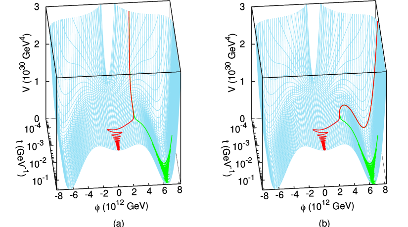
Figure 2: The three dimensional plot of the full curvaton potential $V(\phi)$ versus $\phi$ and $t$ for $\lambda=10^{-4}$. The green (red) line in (a) depicts the path followed by $\phi$ if $\phi_{f}$ is a little above (below) the lower boundary of the 1rst band, while the green (red) line in (b) corresponds to the field evolution if $\phi_{f}$ is a little below (above) the upper boundary of the same band.

In order to get a feeling of the post-inflationary evolution patterns of $\phi$ in the various bands, let us first consider that $\phi_{f}$ is slightly above (below) the lower boundary of the 1rst band which lies at $\phi_{f}\simeq 2.83\times 10^{12}~{}{\rm GeV}$ for $\lambda=10^{-4}$. The interesting part of the path followed by $\phi$ is depicted in Fig. 2a by a green (red) line. The field is initially overdamped and decreases monotonically at a very slow pace. For $t\gtrsim 2\gamma/3m_{3/2}\simeq 2.22\times 10^{-4}~{}{\rm GeV}^{-1}$, $\phi$ is found to lie slightly above (below) $\phi_{\rm max}\simeq 2.61\times 10^{12}~{}{\rm GeV}$. For $t\gtrsim 2/3m_{3/2}\simeq 2.22\times 10^{-3}~{}{\rm GeV}^{-1}$, $H\lesssim m_{3/2}$ and the system becomes underdamped. It falls towards the PQ vacuum at $\phi=f_{a}$ (the trivial false vacuum) and starts performing damped oscillations about it. Soon after this, the universe enters into the radiation dominated era which follows reheating and the damped oscillations of $\phi$ continue until this field finally decays. For $\phi_{f}\lesssim 2.83\times 10^{12}~{}{\rm GeV}$, which corresponds to the zeroth (white) band, the field always rolls monotonically towards the false vacuum at zero and, eventually, is set in damped oscillations about it.

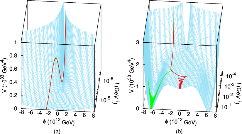
Figure 3: The PQ field evolution for $\phi_{f}$ near the lower boundary of the 3rd (green) band and with $\lambda=10^{-4}$. The green (red) line corresponds to $\phi_{f}$ being slightly above (below) this boundary. The earlier evolution is shown in (a), while the later one in (b).

In Fig. 2b, we show the red (green) path followed by the field $\phi$, if $\phi_{f}$ is taken to lie slightly above (below) the upper boundary of the 1rst band at $\phi_{f}\simeq 3.11\times 10^{13}~{}{\rm GeV}$ for $\lambda=10^{-4}$. We see that the field, as it decreases slowly, passes from the PQ vacuum at $\phi=f_{a}$ and then climbs up the potential until it reaches a value slightly below (above) $\phi_{\rm max}$. It stays there for some time and, finally, falls towards the trivial vacuum (the PQ vacuum at $\phi=f_{a}$) and performs damped oscillations about it. For $2.83\times 10^{12}~{}{\rm GeV}\lesssim\phi_{f}\lesssim 3.11\times 10^{13}~{}{\rm GeV}$, which corresponds to the 1rst (green) band, the field always rolls slowly directly into the PQ vacuum at $\phi=f_{a}$ and oscillates about it. We should note that the upper limit of the ‘quantum’ regime $\phi_{Q}$, which turns out to be $\simeq 9.41\times 10^{12}~{}{\rm GeV}$ (see Eq. (16)), lies is this band for the range of $\lambda$ considered here.

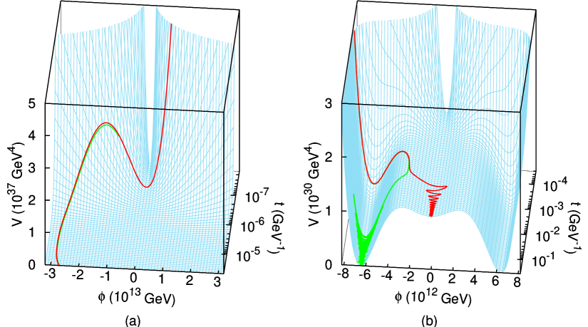
Figure 4: The PQ field evolution for $\phi_{f}$ near the upper boundary of the 3rd (green) band and with $\lambda=10^{-4}$. The green (red) line corresponds to $\phi_{f}$ being slightly below (above) this boundary. The earlier evolution is shown in (a), while the later one in (b).

In Fig. 3, we present the evolution of the field $\phi$ when $\phi_{f}$ happens to lie near the lower boundary of the 3rd (green) band at $\phi_{f}\simeq 2.5\times 10^{16}~{}{\rm GeV}$ again for $\lambda=10^{-4}$. The green (red) line corresponds to $\phi_{f}$ being slightly above (below) this boundary. The earlier evolution of the PQ field is depicted in Fig. 3a. We see that, well before the appearance of the non-trivial minima, the field rolls down slowly, reaches the trivial vacuum and then passes to negative values slowly climbing up the potential. It is, eventually, stabilized for some time slightly after (before) $-\phi_{\rm max}$ and finally falls into the PQ vacuum at $\phi=-f_{a}$ (trivial vacuum) as is obvious from Fig. 3b, where the subsequent evolution is shown. We find that, for $3.11\times 10^{13}~{}{\rm GeV}\lesssim\phi_{f}\lesssim 2.5\times 10^{16}~{}{\rm GeV}$, which corresponds to the 2nd (white) band, the field always falls into the trivial vacuum and oscillates about it.

Fig. 4 shows the green (red) trajectory followed by $\phi$ for $\phi_{f}$ slightly below (above) the upper boundary of the 3rd band at $\phi_{f}\simeq 4.48\times 10^{16}~{}{\rm GeV}$ for $\lambda=10^{-4}$. We see that the slowly moving field passes from zero, overtakes $-f_{a}$, falls back to the PQ minimum at $\phi=-f_{a}$, which has appeared by that time, climbs up to a point slightly below (above) $-\phi_{\rm max}$ and stays there for a period of time. It then falls towards the PQ minimum at $\phi=-f_{a}$ (the trivial minimum) and is set in damped oscillations. Our numerical results show that, for $2.5\times 10^{16}~{}{\rm GeV}\lesssim\phi_{f}\lesssim 4.48\times 10^{16}~{}{\rm GeV}$, which corresponds to the 3rd (green) band, the field always falls into the PQ vacuum at $\phi=-f_{a}$ and oscillates about it. More complicated patterns of evolution of the PQ field are encountered in the higher bands, but we will not discuss them in any detail since these bands are both physically meaningless and useless for our purposes as already explained.

It is interesting to note that the 2nd (white) band extends over almost three orders of magnitude in $\phi_{f}$ and, thus, pushes the 3rd (green) band to large values of $\phi_{f}$. Also, the lower bound on $\phi_{f}$ from the isocurvature perturbation is quite sizeable. The combined effect of these two facts is that the $\phi_{f}$’s which can be useful for our purposes are fairly large. As a consequence, the relative perturbation, $\delta\phi/\phi$, acquired by the curvaton during inflation is somewhat small. This leads to a small partial curvature perturbation, $\zeta_{\phi}$, carried by the oscillating PQ field at the time of its decay. So, as can be seen from Eq. (25), a relatively large $f_{\rm dec}$ is required in order to achieve the COBE constraint on the total curvature perturbation, which makes our task a little tougher. The situation would have certainly been less tight if the 1rst (green) band could be used.

One way to understand the fact that the 2nd band comes out so wide is the following. Consider the classical equation of motion in Eq. (14) during the last part of the period of inflaton oscillations where the induced mass in Eq. (12) can be neglected. For small enough $\phi$’s, the potential $V(\phi)$ can be approximately taken to be quadratic and this equation becomes of the Emden type

$$\ddot{\phi}+\frac{2}{t}\dot{\phi}+m_{3/2}^{2}\phi=0.$$ (36)

The solution of this equation is

$$\phi=\frac{A}{t}\sin m_{3/2}(t-t_{0}),$$ (37)

where $A$ and $t_{0}$ are constants depending on the initial conditions. For $A<0$ and $0<m_{3/2}t_{0}\sim 1$, the field initially (i.e. for $t\lesssim m_{3/2}^{-1}\sim t_{0}$) decreases approximately as $-A\sin m_{3/2}t_{0}/t$. However, as $t$ exceeds $m_{3/2}^{-1}\sim t_{0}$, it is set in damped oscillations about zero. On the other hand, for $A<0$ and $0<m_{3/2}t_{0}\ll 1$, the field initially decreases and reaches zero at $t=t_{0}$. It then passes to negative values and is stabilized for a while (i.e. for $t_{0}\lesssim t\lesssim m_{3/2}^{-1}$) around $Am_{3/2}<0$. It, finally, falls back into zero and starts performing damped oscillations about it. The former behavior is encountered when $\phi_{f}$ lies in the lower part of the 2nd band, while the latter when $\phi_{f}$ reaches the upper part of this band. We see that, in the latter case, the field $\phi$, as it climbs up the potential towards the maximum at $\phi=-\phi_{\rm max}$, ‘breaks’ and enters for a while in a plateau. This makes it more difficult for $\phi$ to reach this maximum. Thus, the upper boundary of the 2nd band is pushed to higher values.

5.3 The inflationary perturbation of the curvaton

We are now ready to discuss the evolution of the inflationary perturbation of $\phi$ and estimate numerically the resulting partial curvature perturbation $\zeta_{\phi}$ at curvaton decay. For any value of $\lambda$ in the range $10^{-4}-10^{-3}$, we take two values of $\phi$ at the end of inflation: $\phi_{f}$ and $\phi_{f}+\delta\phi$ ($\delta\phi=H_{\rm infl}/2\pi$) both lying in the 3rd band and follow numerically their evolution. (Recall that $\delta\phi$ is tiny compared with the width of this band.) For both these initial values, the field ends up performing damped oscillations about the PQ vacuum at $\phi=-f_{a}$. When the amplitude $\phi_{0}$ of these oscillations is adequately reduced, the oscillations become harmonic with their amplitudes differing by an amount $\delta\phi_{0}$. The partial curvature perturbation $\zeta_{\phi}$ is then stabilized to the limiting value $2\,\delta\phi_{0}/3\phi_{0}$, as shown in section 4. This occurs well before the curvaton decay in all the cases which we considered. We find numerically the limiting $\zeta_{\phi}$ for $10^{-4}\leq\lambda\leq 10^{-3}$ and any $\phi_{f}$ in the 3rd band.

It should be mentioned in passing that, for a scalar field with a positive power-law potential and a subdominant energy density in a matter (radiation) dominated universe, Eq. (14) possesses [50] an exact scaling solution, which behaves as a stable attractor provided that the power is greater than 6 (10). In this case, the field is eventually trapped in the attractor and its energy density decreases relative to the dominant matter (radiation) energy density as time elapses. Moreover, any primordial perturbations in this field are washed out since the field falls in the same attractor no matter what its initial conditions were. Consequently, under these circumstances, the field could not play the role of a curvaton since the limiting $\zeta_{\phi}$ would come out tiny. Fortunately, all the powers involved in our PQ potential in Eq. (7) are less than or equal to 6 and, thus, no attractor type behavior is encountered with this potential as our numerical findings also clearly show. Furthermore, if our full potential $V(\phi)$ in Eq. (13) is dominated by the variable induced mass in Eq. (12), new scaling type solutions appear [17]. However, the initial perturbations are not washed out in this case.

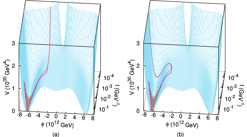
Figure 5: The evolution of the field $\phi$ for two $\phi_{f}$’s differing by a small amount and lying in the 3rd band near its (a) lower, or (b) upper boundary at $\lambda=10^{-4}$. The magenta (brown) field paths correspond to $\phi_{f}$ being nearer (further from ) this boundary. The maximum at $\phi=-\phi_{\rm max}$ acts as a ‘tachyonic amplifier’ of the difference between the fields.

As already indicated, the limiting $\zeta_{\phi}$ comes out generally small. However, if $\phi_{f}$ is near the upper or lower boundary of the 3rd band, $\zeta_{\phi}$ can be enhanced considerably. To see this, let us consider two $\phi_{f}$’s slightly above (below) the lower (upper) boundary of this band which differ by a small amount $\delta\phi$. We take again $\lambda=10^{-4}$. The relevant parts of the resulting field paths are shown in Fig. 5a (Fig. 5b). The magenta path corresponds to the $\phi_{f}$ which is nearer the boundary, while the brown one to the $\phi_{f}$ furthermost from the boundary. We observe that the ‘magenta field’ is stabilized nearer the maximum at $\phi=-\phi_{\rm max}$ than the ‘brown field’ after its first slow (its slow return from its first slow) oscillation to negative values. Then, due to the flatness of the potential around the maximum, the ‘magenta field’ remains near the maximum longer than the ‘brown field’. Consequently, it falls towards the PQ minimum at $\phi=-f_{a}$ with a relative delay and, thus, the gap $\delta\phi$ between the fields increases considerably. This leads to a sizeable enhancement of the disparity in the amplitudes of the subsequent damped oscillations of the two fields about the minimum.

We see that the local maxima can act as ‘tachyonic amplifiers’ of the curvaton perturbation which originates from inflation. Note, however, that the amplification happens only if $\phi_{f}$ is close to the boundary of the band and only once during the field evolution, since, at subsequent times, the field never approaches the local maxima again. This effect is crucial for the viability of our model since otherwise the limiting $\zeta_{\phi}$ turns out too small. It should be mentioned that an amplification of perturbations while the field is near a local maximum of the potential was also encountered in Ref. [51]. However, the phenomenon there was of a quantum nature referring to the quantum perturbations of the inflaton in de Sitter space. In our case, the effect is completely classical and takes place well after the termination of inflation.

5.4 The curvaton decay

We now turn to the discussion of the curvaton decay and the evaluation of the final curvature perturbation. The curvaton decays into a pair of Higgsinos via the second coupling in the superpotential of Eq. (2). This same coupling is also responsible for the $\mu$-term. Of course, for this decay to be kinematically possible, we must make sure that the Higgsino mass $\mu=\beta f_{a}^{2}/4m_{P}$ does not exceed half of the curvaton mass which is given by

$$m_{\phi}^{2}=V_{\rm PQ}^{\prime\prime}(\phi=\pm f_{a})=\frac{1}{3}\sqrt{|A|^{2}-12}\left(|A|+\sqrt{|A|^{2}-12}\right)m_{3/2}^{2}.$$ (38)

This mass is $\lambda$-independent and equals about $965~{}{\rm GeV}$ for the input numbers used. The curvaton decay time $t_{\phi}=\Gamma_{\phi}^{-1}$, where $\Gamma_{\phi}$ is the curvaton decay width given by

$$\Gamma_{\phi}=\frac{\beta^{2}f_{a}^{2}}{8\pi m_{P}^{2}}m_{\phi}.$$ (39)

We take $\mu=300~{}{\rm GeV}$, which yields $\beta\simeq 0.697\lambda$ and $t_{\phi}\simeq 7.6~{}\lambda^{-1}\times 10^{13}~{}{\rm GeV}^{-1}$.

It is important to ensure that the coherently oscillating curvaton field does not evaporate [52] as a result of scattering with particles in the thermal bath before it decays into Higgsinos. During the period between the onset of field oscillations about a PQ vacuum and roughly the electroweak phase transition, the Higgs superfields are in equilibrium with the thermal bath and could knock the PQ field out of the zero mode. The dominant process is the Higgsino-curvaton scattering through the second coupling in the RHS of Eq. (2). The cross section is $\sigma\sim\beta^{2}/m_{P}^{2}$, which yields the thermal decay rate $\Gamma_{\rm th}\sim\beta^{2}T^{3}/m_{P}^{2}$. Avoidance of evaporation then requires that $\beta^{2}T^{3}/m_{P}^{2}\lesssim H$. Before (after) reheating, $H\sim T^{4}/m_{P}T_{\rm reh}^{2}$ [39] ($H\sim T^{2}/m_{P}$) and this requirement becomes $T\gtrsim\beta^{2}T_{\rm reh}^{2}/m_{P}$ ($T\lesssim m_{P}/\beta^{2}$), which is well-satisfied.

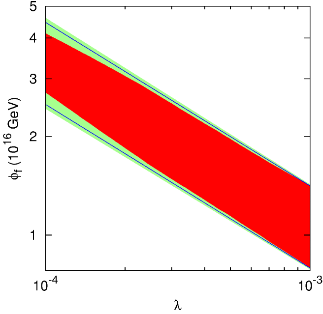
Figure 6: The 3rd band (all the colored area) with the blue solution lines on which the COBE constraint $\zeta=5\times 10^{-5}$ is satisfied. The green (red) area of the band is allowed (excluded) by the non-Gaussianity bound from the WMAP satellite.

The energy density of the oscillating curvaton at $t_{\phi}$ is evaluated numerically for each $\phi_{f}$ in the 3rd band and each $\lambda$ in the range $10^{-4}-10^{-3}$. From Eq. (24), we can then calculate $f_{\rm dec}$, the fraction $f$ at curvaton decay. The final curvature perturbation $\zeta$ is estimated, in the instantaneous decay approximation, by multiplying this fraction by the limiting $\zeta_{\phi}$ (see Eq. (25)). The result is put equal to $5\times 10^{-5}$ as required by COBE [29]. We find that there are two solutions for each $\lambda$, one close to the lower boundary of the band and the other close to the upper boundary. These solutions lie on the two blue lines in Fig. 6, where the green and red areas together constitute the 3rd band. It is true that the solutions turn out to be quite close to the boundaries of the band. This means that the ‘tachyonic amplification’ of the inflationary perturbation in the curvaton field, which occurs near a maximum of the potential, plays a crucial role. On the other hand, the gap between the solutions and the boundaries is not so tiny as to imply that the solutions are finely tuned. Moreover, this gap is huge compared to the inflationary perturbation $\delta\phi\simeq 3.14\times 10^{10}~{}{\rm GeV}$.

We already stressed that, in the curvaton scenario, significant non-Gaussianity of the curvature perturbation appears if the curvaton decays before dominating the energy density of the universe. The recent CMBR data from the WMAP satellite yield [6] an upper bound on the possible non-Gaussianity in the curvature perturbation. This bound implies [11] that, at $95\%$ c.l., the fraction $f_{\rm dec}\gtrsim 9.33\times 10^{-3}$. The corresponding allowed (excluded) area of the 3rd band is colored green (red) in Fig. 6. We see that the (blue) solution lines lie totally in the green area and, thus, are fully consistent with the negative results of the WMAP satellite on non-Gaussianity.

As already explained, if $\phi_{f}$ lies in a green band and near one of its boundaries, the PQ field, before starting its damped oscillations about a PQ vacuum, stays for a while near a maximum of the potential. This ‘tachyonic effect’ is also important for the fulfillment of the non-Gaussianity constraint. Indeed, it causes a delay in the commencement of the damped oscillations of $\phi$ and, thus, leads to a larger $\rho_{\phi}$ at curvaton decay. Therefore, the fraction $f_{\rm dec}$ is enhanced. As a consequence, the non-Gaussianity bound can be satisfied provided that $\phi_{f}$ is adequately close to the boundaries of the band. This explains the fact that the green area in Fig. 6 extends near the boundaries of the band. Needless to say that the enhancement of $f_{\rm dec}$ also facilitates the fulfillment of the COBE constraint on the curvature perturbation.

In summary, we conclude that, in the investigated scheme which simultaneously solves the strong CP and $\mu$ problems, the PQ field can successfully and naturally act as a curvaton with all the relevant cosmological requirements satisfied.

6 Conclusions

We considered a minimal extension of MSSM which simultaneously solves the strong CP and $\mu$ problems via a PQ and a continuous R symmetry. This model can be readily embedded in simple and natural SUSY GUTs which incorporate the hybrid inflationary scenario and generate the observed baryon asymmetry of the universe through a primordial leptogenesis. We, thus, took the model supplemented with hybrid inflation and leptogenesis, but without committing ourselves to the specific details of these scenarios.

We examined whether, in this model, the PQ field can play the role of the curvaton generating the primordial density perturbations which are needed for explaining the structure formation in the universe and the observed anisotropies in the CMBR. A crucial requirement is that the PQ field is light during the last $50-60$ inflationary e-foldings so that it receives a superhorizon spectrum of perturbations from inflation. This condition can be easily satisfied in our model with global SUSY, where the PQ potential is almost flat, provided that, during inflation, the value of the PQ field is not too large. We must, though, employ some mechanism which can prevent the lifting of the flatness of the potential by the SUGRA corrections during inflation.

We followed the evolution of the PQ field after the end of inflation under the assumption that the SUSY breaking corrections to its potential from the finite energy density of the early universe are somewhat small. We found that the field, after an initially slow evolution, is set in damped oscillations about zero or one of the PQ vacua, depending on its value right after inflation. More precisely, the values of the PQ field at the end of inflation can be classified into successive bands which lead to the trivial or the PQ vacua in turn. Needless to say that only the bands leading to one of the PQ vacua are useful for our purposes.

In our model, as it turns out, the bulk of the CDM in the universe consists of axions which are produced at the QCD phase transition. They carry an isocurvature perturbation which is uncorrelated with the total curvature perturbation generated by the PQ field. The rest of CDM is made of LSPs (lightest neutralinos) which originate from the late decay of the primordial gravitinos produced thermally at reheating. These neutralinos as well as the baryons, which are assumed to come from a primordial leptogenesis that took place at reheating, acquire an isocurvature perturbation fully correlated with the curvature perturbation. So, the overall isocurvature perturbation has a mixed correlation with the total curvature perturbation. We found that the presently available restriction on such an isocurvature perturbation from the CMBR and other data excludes the lowest lying band which leads to a PQ vacuum. High order bands are also excluded since they do not fulfill the condition that the curvaton is light during inflation. We are, finally, left with only one allowed band leading to a PQ vacuum. We, thus, focus our attention to this particular band.

The inflationary perturbation of the PQ field evolves as the cosmic time elapses after the end of inflation and, when the PQ field is set in harmonic oscillations about a PQ vacuum, yields a stable perturbation in the energy density of this field. At the decay of the PQ field, the perturbation is transferred to the radiation dominated plasma generating the total curvature perturbation. We found that the COBE constraint on the total curvature perturbation can be naturally fulfilled provided that we are somewhat near the boundaries of the band. An important phenomenon, which allows us to achieve this, is the ‘tachyonic amplification’ of the original inflationary perturbation in the PQ field as this field is temporarily stabilized near a local maximum of the potential.

Finally, we imposed the bound on the possible non-Gaussianity of the total curvature perturbation from the recent CMBR data obtained by the WMAP satellite. We saw that, although the bulk of the band is excluded by this constraint, the COBE requirement is still fully consistent with it. The ‘tachyonic effect’, i.e. the fact that the field hangs around a maximum of the potential for a period of time if its value right after inflation is close to the boundaries of the band, is crucial for having the non-Gaussianity requirement satisfied. The reason is that, due to this effect, the commencement of the damped field oscillations is delayed and, thus, the density fraction of the curvaton is enhanced. This also facilitates the achievement of the COBE constraint on the curvature perturbation.

In conclusion, we have shown that, in our scheme, which naturally and simultaneously solves the $\mu$ and strong CP problems, the PQ field can successfully play the role of the curvaton generating the total curvature perturbation in the universe in accord with the COBE measurements. The bounds on the isocurvature perturbation and non-Gaussianity from the available CMBR data can also be satisfied.