The behaviour of the transverse momentum fluctuations with the centrality of the collision shown by the Relativistic Heavy Ion Collider data is naturally explained by the clustering of color sources. In this framework, elementary color sources –strings– overlap forming clusters, so the number of effective sources is modified. These clusters decay into particles with mean transverse momentum that depends on the number of elementary sources that conform each cluster, and the area occupied by the cluster. The transverse momentum fluctuations in this approach correspond to the fluctuations of the transverse momentum of these clusters, and they behave essentially as the number of effective sources.

PACS: 25.75.Nq, 12.38.Mh, 24.85.+p

Event-by-event fluctuations of the mean transverse momentum are considered to be one of the most important tools to identify a phase transition in the evolution of the system created in relativistic heavy ion collisions, since a second order phase transition may lead to a divergence of the specific heat which could be observed as fluctuations in mean transverse momentum [1]-[3]. These fluctuations have been extensively studied both theoretically [4]-[10] and experimentally [11]-[17]. Recently, the PHENIX collaboration [15]-[16] of the Relativistic Heavy Ion Collider (RHIC) has reported a peculiar behaviour of the variable $F_{p_{T}}$ that measures the transverse momentum fluctuations as a function of the number of participants in Au-Au collisions. $F_{p_{T}}$ quantifies the deviation of the observed fluctuations from statistically independent particle emission,

$$F_{p_{T}}=\frac{\omega_{data}-\omega_{random}}{\omega_{random}}$$ (1)

where

$$\omega=\frac{\sqrt{<p_{T}^{2}>-<p_{T}>^{2}}}{<p_{T}>}\ ,$$ (2)

and $<p_{T}>$ is the mean transverse momentum averaged over all particles and all events. The data show that $F_{p_{T}}$ increases with the number of participants, reaching a maximum around $N_{part}=150\div 200$ and decreasing at higher centrality. In this paper we show that this behaviour is naturally explained by the clustering of elementary color sources that may take place in heavy ion collisions.

Multiparticle production is currently described in terms of color strings stretched between the partons of the projectile and the target. These strings decay into new ones by sea $q-\bar{q}$ production, and subsequently hadronize to produce the observed hadrons. In our approach, the strings are equivalent to effective color sources with a fixed tranverse size $\pi r_{0}^{2}$, with $r_{0}\simeq 0.2$ fm, filled with the color field created by the colliding partons. With increasing energy and/or atomic number of the colliding nuclei, the number of exchanged strings grows, so they start to interact forming clusters. In the transverse space that means that the transverse areas of the strings overlap, as it happens for disks in the two dimensional percolation theory. Moreover, at a certain critical density of disks, $\eta\simeq 1.12-1.18$, a macroscopical cluster appears which marks the percolation phase transition [18]-[19], which is a second order, non thermal, phase transition.

In the case of a nuclear collision, the density of disks –elementary strings– corresponds to

$$\eta_{c}=\frac{N_{s}S_{1}}{S_{A}}$$ (3)

where $N_{s}$ is the total number of strings created in the collision, each one of an area $S_{1}=\pi r_{0}^{2}$, and $S_{A}$ corresponds to the nuclear overlap area, $S_{A}=\pi R^{2}_{A}$ for central collisions.

The percolation theory governs the geometrical pattern of the string clustering. Its observable implications, however, required the introduction of some dynamics in order to describe the behaviour of the cluster formed by several overlapping strings [20]-[21]. We assume that a cluster of $n$ strings that occupies an area $S_{n}$ behaves as a single color source with a higher color field, generated by a higher color charge $Q_{n}$. This charge corresponds to the vectorial sum of the color charges of each individual string ${\bf Q}_{1}$. The resulting color field covers the area $S_{n}$ of the cluster. As $Q_{n}^{2}=(\sum_{1}^{n}{\bf Q}_{1})^{2}$, and the individual string colors may be oriented in an arbitrary manner respective to one another, the average ${\bf Q}_{1i}{\bf Q}_{1j}$ is zero, so $Q_{n}^{2}=nQ_{1}^{2}$. $Q_{n}$ depends also on the area $S_{1}$ of each individual string that comes into the cluster, as well as on the total area of the cluster $S_{n}$, $Q_{n}=\sqrt{nS_{n}\over S_{1}}Q_{1}$ . We take $S_{1}$ constant and equal to a disk of radius $r_{0}\simeq 0.2$ fm. $S_{n}$ corresponds to the total area occupied by $n$ disks [20]. One could do reasonable alternative assumptions about the interaction among the strings, but they have incompatibilities with correlation data [22]-[23].

Notice that if the strings are just touching each other, $S_{n}=nS_{1}$ and $Q_{n}=nQ_{1}$, so the strings behave independently. On the contrary, if they fully overlap, $S_{n}=S_{1}$ and $Q_{n}=\sqrt{n}Q_{1}$. Knowing the color charge $Q_{n}$, one can compute the multiplicity $\mu_{n}$ and the mean transverse momentum $<p_{T}>_{n}$ of the particles produced by a cluster of $n$ strings. According to the Schwinger mechanism for the fragmentation of the cluster, one finds

$$\mu_{n}=\sqrt{\frac{nS_{n}}{S_{1}}}\mu_{1}\ {\rm and}\ <p_{T}>_{n}=\Big{(}\frac{nS_{1}}{S_{n}}\Big{)}^{1/4}<p_{T}>_{1}$$ (4)

for the multiplicity $\mu_{n}$ and the average transverse momentum $<p_{T}>_{n}$ of the particles produced by a cluster formed by $n$ strings, where $\mu_{1}$ and $<p_{T}>_{1}$ correspond to the mean multiplicity and the mean transverse momentum of the particles produced by one individual string. These equations constitute the main tool of our evaluations.

The behaviour of the transverse momentum fluctuations can be understood as follows: At low density, most of the particles are produced by individual strings with the same $<p_{T}>_{1}$, so the fluctuations are small. Similarly, at large density above the percolation critical point, there is essentially only one cluster formed by most of the strings created in the collision and therefore fluctuations are not expected either. Instead, the fluctuations are expected to be maximal below the percolation critical density, where the number of clusters is larger. Moreover, there are clusters formed by very different numbers of strings, with different size, and therefore with different $<p_{T}>_{n}$.

In order to develop quantitatively this idea, we introduce the function [4] $\phi$ defined by

$$\phi=\sqrt{\frac{<Z^{2}>}{<\mu>}}-\sqrt{<z^{2}>}\ .$$ (5)

$F_{p_{T}}$ is related to $\phi$ [14], approximately

$$F_{p_{T}}=\frac{\phi}{\sqrt{<z^{2}>}}=\frac{1}{\sqrt{<z^{2}>}}\sqrt{\frac{<Z^{2}>}{<\mu>}}-1\ .$$ (6)

For each particle we define $z_{i}={p_{T}}_{i}-<p_{T}>$, where ${p_{T}}_{i}$ is the transverse momentum of the particle $i$ and $<p_{T}>$ is the mean transverse momentum of all particles averaged over all events. $\sqrt{<z^{2}>}$ is the second moment of the single particle inclusive $z$ distribution, and it is averaged over all events. $Z$ is defined for each event,

$$Z_{i}=\sum_{j=1}^{N_{i}}z_{j}$$ (7)

where $N_{i}$ is the number of particles produced in an event $i$.

In this way, introducing our formulae for the multiplicity and the mean $p_{T}$ we get:

$$<p_{T}>=\frac{\sum_{i=1}^{N_{events}}\sum_{j}\mu_{{n_{j}}}<p_{T}>_{{n_{j}}}}{\sum_{i=1}^{N_{events}}\sum_{j}\mu_{{n_{j}}}}\ .$$ (8)

The sum over $j$ goes over all individual clusters $j$, each one formed by ${{n_{j}}}$ strings and occupying an area $S_{{n_{j}}}$. The quantities ${{n_{j}}}$ and $S_{{n_{j}}}$ are obtained for each event, using a Monte Carlo code [24]-[25], based on the quark gluon string model. Each string is generated at an identified impact parameter in the transverse space. Knowing the tranverse area of each string, we identified all the clusters formed in each event, the number of strings ${{n_{j}}}$ that conforms each cluster $j$, and the area occupied by each cluster $S_{{n_{j}}}$. Note that for two different clusters, $j$ and $k$, formed by the same number of strings ${{n_{j}}}=n_{k}$, the areas $S_{{n_{j}}}$ and $S_{n_{k}}$ can vary. Because of this we do the sum over all individual clusters.

For the quantities $<p_{T}>_{{n_{j}}}$ –mean $p_{T}$ of the particles produced by a cluster $j$ of ${n_{j}}$ strings and area $S_{{n_{j}}}$– and $\mu_{{n_{j}}}$ –mean multiplicity of a cluster $j$ formed by ${n_{j}}$ strings and of area $S_{{n_{j}}}$– we apply the analytical expressions given by eqs. (4). Finally we do the average over all events.

By introducing eqs. (4) for $<p_{T}>_{{n_{j}}}$ and $\mu_{{n_{j}}}$ we get:

$$<p_{T}>=\frac{\sum_{i=1}^{N_{events}}\sum_{j}\Big{(}\frac{{n_{j}}S_{n_{j}}}{S_{1}}\Big{)}^{1/2}\mu_{1}\Big{(}\frac{{n_{j}}S_{1}}{S_{n_{j}}}\Big{)}^{1/4}<p_{T}>_{1}}{\sum_{i=1}^{N_{events}}\sum_{j}\Big{(}\frac{{n_{j}}S_{n_{j}}}{S_{1}}\Big{)}^{1/2}\mu_{1}}$$ (9)

$$=\frac{\Big{<}\sum_{j}{n_{j}}^{3/4}(\frac{S_{n_{j}}}{S_{1}})^{1/4}\Big{>}}{\Big{<}\sum_{j}(\frac{{n_{j}}S_{n_{j}}}{S_{1}})^{1/2}\Big{>}}<p_{T}>_{1}$$ (10)

$$=f_{2}<p_{T}>_{1}$$ (11)

where the mean value in the r.h.s. corresponds to an average over all events.

For the quantities $<z^{2}>$ and $<Z^{2}>$ we obtain:

$$<z^{2}>=\frac{\sum_{i=1}^{N_{events}}\sum_{j}\Big{(}\frac{{n_{j}}S_{n_{j}}}{S_{1}}\Big{)}^{1/2}\mu_{1}\Big{[}\Big{(}\frac{{n_{j}}S_{1}}{S_{n_{j}}}\Big{)}^{1/4}<p_{T}>_{1}-<p_{T}>\Big{]}^{2}}{\sum_{i=1}^{N_{events}}\sum_{j}\Big{(}\frac{{n_{j}}S_{n_{j}}}{S_{1}}\Big{)}^{1/2}\mu_{1}}$$ (12)

$$=\Big{[}\frac{\Big{<}\sum_{j}{n_{j}}\Big{>}}{\Big{<}\sum_{j}(\frac{{n_{j}}S_{n_{j}}}{S_{1}})^{1/2}\Big{>}}-f_{2}^{2}\Big{]}<p_{T}>_{1}^{2}$$ (13)

$$=(f_{1}-f_{2}^{2})<p_{T}>_{1}^{2}$$ (14)

and

$$\frac{<Z^{2}>}{<\mu>}=\frac{\sum_{i=1}^{N_{events}}\Big{[}\sum_{j}\Big{(}\frac{{n_{j}}S_{n_{j}}}{S_{1}}\Big{)}^{1/2}\mu_{1}\Big{[}\Big{(}\frac{{n_{j}}S_{1}}{S_{n_{j}}}\Big{)}^{1/4}<p_{T}>_{1}-<p_{T}>\Big{]}\Big{]}^{2}}{\sum_{i=1}^{N_{events}}\sum_{j}\Big{(}\frac{{n_{j}}S_{n_{j}}}{S_{1}}\Big{)}^{1/2}\mu_{1}}$$ (15)

$$=\Big{[}\frac{\Big{<}\Big{[}\sum_{j}{n_{j}}^{3/4}\Big{(}\frac{S_{n_{j}}}{S_{1}}\Big{)}^{1/4}\Big{]}^{2}\Big{>}}{\Big{<}\sum_{j}\Big{(}\frac{{n_{j}}S_{n_{j}}}{S_{1}}\Big{)}^{1/2}\Big{>}}+$$ (16)

$$+\frac{\Big{<}\Big{[}\sum_{j}\Big{(}\frac{{n_{j}}S_{n_{j}}}{S_{1}}\Big{)}^{1/2}\Big{]}^{2}\Big{>}}{\Big{<}\sum_{j}\Big{(}\frac{{n_{j}}S_{n_{j}}}{S_{1}}\Big{)}^{1/2}\Big{>}}f_{2}^{2}-\frac{\Big{<}\sum_{j}{n_{j}}^{3/4}\Big{(}\frac{S_{n_{j}}}{S_{1}}\Big{)}^{1/4}\sum_{j}\Big{(}\frac{{n_{j}}S_{n_{j}}}{S_{1}}\Big{)}^{1/2}\Big{>}}{\Big{<}\sum_{j}\Big{(}\frac{{n_{j}}S_{n_{j}}}{S_{1}}\Big{)}^{1/2}\Big{>}}2f_{2}\Big{]}\mu_{1}<p_{T}>_{1}^{2}$$ (17)

$$=[f_{3}+f_{4}f_{2}^{2}-2f_{2}f_{5}]\mu_{1}<p_{T}>_{1}^{2}\ .$$ (18)

Finally we arrive to:

$$F_{p_{T}}=\sqrt{\mu_{1}}\sqrt{\frac{f_{3}+f_{4}f_{2}^{2}-2f_{2}f_{5}}{f_{1}-f_{2}^{2}}}-1\ .$$ (19)

where $f_{1}$, $f_{2}$, $f_{3}$, $f_{4}$ and $f_{5}$ are defined in the expressions (9)-(11).

In order to compute eq. (12), several ingredients are necessaries. On one hand we need a Monte Carlo code [24]-[25] for the cluster formation, in order to compute the number of strings that come into each cluster and the area of the cluster. On the other hand, we do not use a Monte Carlo code for the decay of the cluster, since we apply analytical expressions (eqs. (4)) for the transverse momentum and the multiplicities of the clusters.

We also need the value of $\mu_{1}$ –multiplicity produced by one individual string–. It was previously fixed from a comparison of the model to SPS and RHIC data [20]-[21] on multiplicities. In the first Ref. of [20], the total multiplicity per unit rapidity produced by one string has been taken as $\mu_{0\,{tot}}\simeq 1$. If we assume that $2/3$ of the created particles are charged, that would lead to a charged particle multiplicity per unit rapidity for each individual string of $\mu_{0\,{ch}}=0.65$. In order to compare with experimental data we define $\mu_{1}=\mu_{0\,{ch}}\,y$, where $y$ is the rapidity interval of the produced particles. We don’t introduce any dependence of $\mu_{0}$ with the energy or the centrality of the collision. Notice that in (12) the value of $<p_{T}>_{1}$ cancels.

We have neglected the subsequent rescattering of hadrons and resonances that takes place after the decay of the clusters. It gives rise to correlations which would be similar in the clustering approach and in an independent string picture, unless additional dynamics were taken into account. Therefore its contribution to $F_{p_{T}}$ cancels in our approach.

The comparison of our results for the dependence of $F_{p_{T}}$ on the number of participants $N_{p}$ with the PHENIX data [16] is shown in Fig. 1. The calculation is done for charged particles in the rapidity range $|\eta|<0.35$, $\mu_{1}=0.7\,\mu_{0\,{ch}}$. An acceptable overall agreement is obtained.

In order to compute our value for $F_{p_{T}}$, we take into account all possible transverse momenta, whereas in the experiment there is a limited acceptance, 0.2 GeV/c $<p_{T}<p_{T}^{max}$. PHENIX [15]-[16] has studied the variation of $F_{p_{T}}$ with the maximal value of the acceptance for $p_{T}$, $p_{T}^{max}$. The maximum of $F_{p_{T}}$ is reached for the largest acceptance, $p_{T}^{max}=4$ GeV/c [15]. So we can expect that our value for $F_{p_{T}}$ is going to be higher than the experimental one, specially for a moderate number of participants, $N_{p}$, since the truncated average $p_{T}$ [26], $<p_{T}^{trunc}>=\frac{\int_{p_{T}^{min}}^{\infty}p_{T}dN/dp_{T}}{\int_{p_{T}^{min}}^{\infty}dN/dp_{T}}-p_{T}^{min}$, decreases with the number of participants for $p_{T}^{min}>2$ GeV/c. This means that, for momenta higher than 2 GeV/c, the high $p_{T}$ contribution would be due to collisions with a moderate number of participants. These considerations may explain the difference between our results and PHENIX data –with a limited acceptance of 0.2 GeV/c $<p_{T}<2.0$ GeV/c– at low $N_{p}$.

In Fig. 2 our results for $\phi_{p_{T}}$ of charged particles in Pb-Pb central collisions at 158 AGeV are compared with the experimental data of NA49 Collaboration [27]. In this case the data correspond to the forward rapidity range $4.0<y<5.5$. For this reason we use $\mu_{1}=1.5\,\mu_{0\,{ch}}$, which in principal implicates larger correlations. However we see that this effect is compensated, since we have a lower value for the mean number of strings at fixed $N_{p}$, due to:

a) lower energy at SPS than at RHIC so less strings are produced,

b) the mean number of strings in this rapidity region is proportional to the number of participants $N_{p}$, while in the central region it is proportional to $N_{p}^{4/3}$ due to the contribution of $q-\bar{q}$ strings from the sea.

For the computation of $\phi_{p_{T}}$ we use $<p_{T}>_{1}=0.3$ GeV/c.

The CERES Collaboration has also measured $\phi_{p_{T}}$ [27] at four different centralities: $0-5\%$, $5-10\%$, $10-15\%$ and $15-20\%$ for Pb-Au collisions at 40, 80 and 158 AGeV/c in the central pseudorapidity range $2.2<\eta<2.7$ and restricted to tracks with transverse momenta $0.1<p_{T}<1.5$ GeV/c. Due to the narrower rapidity and transverse momentum range one would expect a lower $\phi_{p_{T}}$ value. However this is compensated with the increase of the number of strings at central rapidities. The data at 158 AGeV, after short range removal, are 3.3, 3.6, 4.4 and 4.1 for the above mentioned centralities, with errors of the order of 1.5 –for smaller energies the data are lower as expected–. These values and their dependence with centrality are compatible with our results of Fig. 2.

In order to have a better understanding of the behaviour of $F_{p_{T}}$ and $\phi_{p_{T}}$ on the number of participants, we plot in Fig. 3 and Fig. 4 the mean number of clusters $M$ and the dispersion on the number of clusters multiplied by the number of clusters $\sigma_{M}*M$ at RHIC and SPS energies. The ratio $\sigma_{M}^{2}/M$ would be one in the case of a Poisson distribution. The $p_{T}$ fluctuations are due in our approach to the different mean transverse momenta of the clusters. These momenta depend on the number of strings that comes into the cluster and the area occupied by the cluster through our eq. (4), therefore $M$ and $\sigma_{M}$ should be the key quantities. However, $\sigma_{M}^{2}/M$ ranges between $1/2$ and 2 in the whole $N_{p}$ range, what indicates a lower variation than the one for $M$, as can be seen from Fig. 3 and 4 where $M$ and $\sigma_{M}*M$ are plotted. The only effect of $\sigma_{M}$ is to shift the maximum of $M$. Because of this we expect the dependence of $F_{p_{T}}$ and $\phi_{p_{T}}$ on $N_{p}$ to be more similar to the $M$ behaviour, as it is actually. In other words, a decrease in the number of effective sources leads to a decrease of the tranverse momentum fluctuations.

Similar conclusions have been reached in Ref. [29], where a formula for $F_{p_{T}}$ as a function of the cluster dispersion over the mean number of strings per cluster has been obtained.

Notice that we only need to know the number of strings formed for each centrality and their location in the impact parameter space in order to form clusters. This information, together with eq. (4), is enough for us to calculate $F_{p_{T}}$ and $\phi_{p_{T}}$. The same variables have been able to describe the behaviour of the strength of two [22] and three [23] body Bose-Einstein correlations with centrality and the dependence of the multiplicities and transverse momentum distributions [21], [28] on the centrality. All that points out that the percolation approach may be appropriate to describe the relativistic heavy ion collisions.

We thank J. Dias de Deus for useful discussions. This work has been done under Contract No FPA2002-01161 from CICYT of Spain and FEDER from EU.

FIG. 1.: $F_{p_{T}}(\%)$ versus the number of participants. Experimental data from PHENIX at $\sqrt{s}=200$ GeV are compared with our results (solid line).

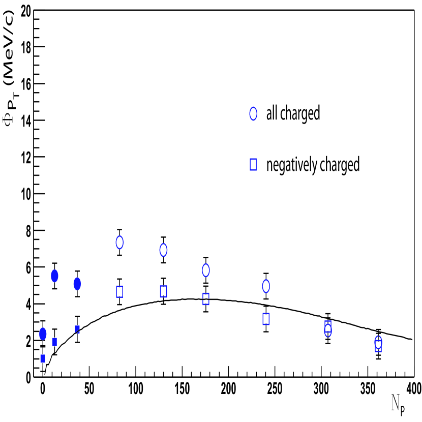
FIG. 2.: $\phi_{p_{T}}$ versus the number of participants. Experimental data from NA49 Collaboration at SPS energies are compared with our results (solid line).

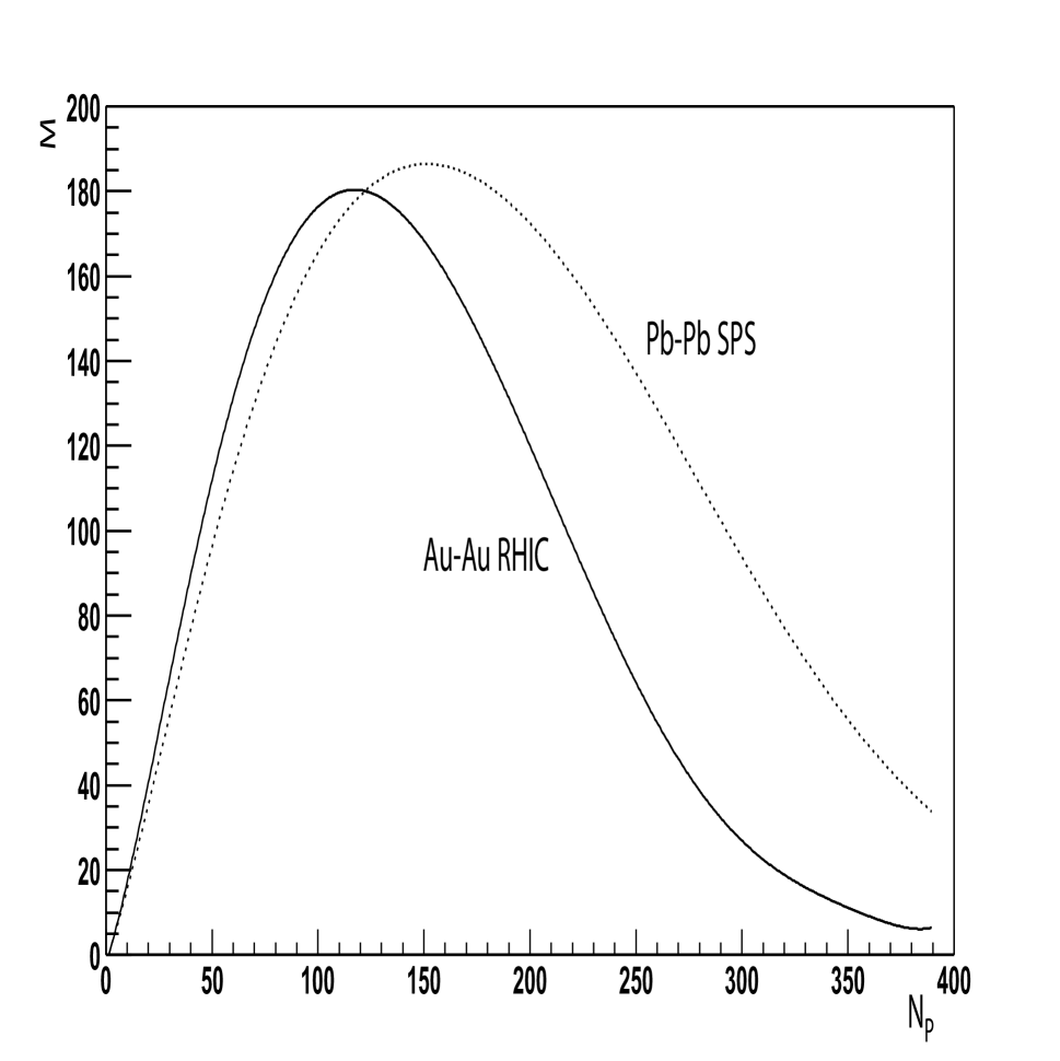
FIG. 3.: Mean number of clusters $M$ versus the number of participants for Pb-Pb collisions at SPS energies (dotted line) and Au-Au collisions at RHIC energies (solid line).

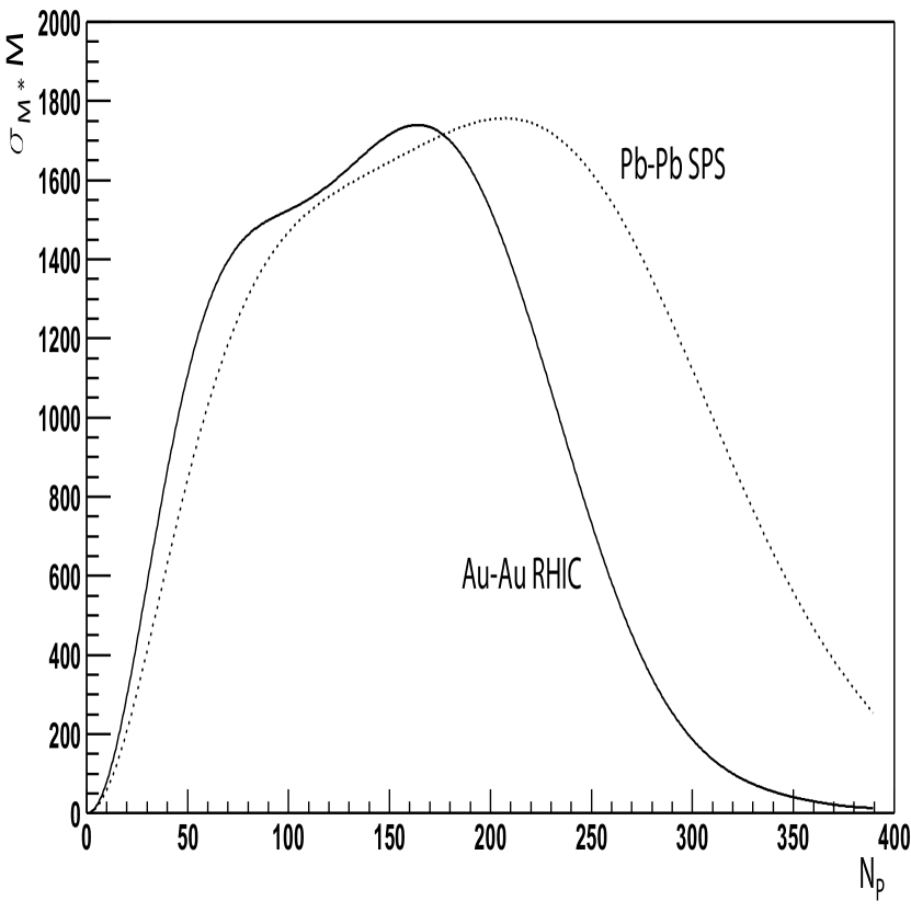
FIG. 4.: Dispersion on the number of clusters multiplied by the number of clusters $\sigma_{M}*M$ versus the number of participants for Pb-Pb collisions at SPS energies (dotted line) and Au-Au collisions at RHIC energies (solid line).

REFERENCES

- [1] L. Stodolsky, Phys. Rev. Lett. 75, 1044 (1995).
- [2] E. Shuryak, Phys. Lett. B430, 9 (1998).
- [3] M. Stephanov, K. Rajagopal and E. Shuryak, Phys. Rev. D60, 114028 (1999).
- [4] M. Gazdzicki and S. Mrowczynski, Z. Phys. C54, 127 (1992).
- [5] S. A. Voloshin, V. Koch and H. Ritter, Phys. Rev. C60, 024901 (1999).
- [6] A. Capella, E. G. Ferreiro and A. B. Kaidalov, Eur. Phys. J. C11, 163 (1999); F. Iin, A. Tai, M. Gazdzicki and R. Stock, Eur. Phys. J. C8, 649 (1999).
- [7] T. A. Trainor, hep-ph/0001148.
- [8] H. Heiselberg, Phys. Rept. 351, 161 (2001).
- [9] W. M. Alberio, A. Lavagno and P. Quarati, Eur. Phys. J. C12, 499 (2000).
- [10] O. V. Utyuzh, G. Wilk and Z. Wlodarczyk, J. Phys. G26, L39 (2000).
- [11] M. J. Tannenbaum, Phys. Lett. B498, 24 (2001).
- [12] NA49 Collaboration, H. Appelshäuser et al., Phys. Lett. B459, 679 (1999).
- [13] CERES Collaboration, H. Appelshäuser et al., Nucl. Phys. A698, 253c (2002).
- [14] PHENIX Collaboration, K. Adcox et al., Phys. Rev. C66, 024901 (2002).
- [15] PHENIX Collaboration, J. Nystrand, Nucl. Phys. A715, 603c (2003).
- [16] PHENIX Collaboration, S. S. Adler et al., nucl-ex/0310005.
- [17] STAR Collaboration, R. L. Ray, Phys. A715, 45c (2003).
- [18] N. Armesto, M. A. Braun, E. G. Ferreiro and C. Pajares, Phys. Rev. Lett. 77, 3736 (1996).
- [19] M. Nardi and H. Satz, Phys. Lett. B442, 14 (1998); J. Dias de Deus, R. Ugoccioni and A. Rodrigues, Eur. Phys. J. C16, 537 (2000); S. Digal, S. Fortunato, P. Petreczky and H. Satz, Phys. Lett. B549, 101 (2002).
- [20] M. A. Braun and C. Pajares, Eur. Phys. J. C16, 349 (2000); Phys. Rev. Lett. 85, 4864 (2001); M. A. Braun, E. G. Ferreiro, F. del Moral and C. Pajares, Eur. Phys. J. C25, 249 (2002).
- [21] M. A. Braun, F. del Moral and C. Pajares, Phys. Rev. C65, 024907 (2002).
- [22] M. A. Braun, F. del Moral and C. Pajares, Eur. Phys. J. C21, 557 (2001); F. del Moral and C. Pajares, Nucl. Phys. B92 (Proc. Suppl.), 95 (2001).
- [23] M. A. Braun, F. del Moral and C. Pajares, Phys. Lett. B551, 291 (2003).
- [24] N. S. Amelin, M. A. Braun and C. Pajares, Z. Phys. C63, 507 (1994).
- [25] N. S. Amelin, N. Armesto, C. Pajares and D. Sousa, Eur. Phys. J. C22, 149 (2001); N. Armesto, C. Pajares and D. Sousa, Phys. Lett. B527, 92 (2002).
- [26] PHENIX Collaboration, K. Adcox et al., Phys. Lett. B561, 82 (2003); PHENIX Collaboration, S. S. Adler et al., nucl-ex/0308006.
- [27] NA49 Collaboration, C. Blume et al., Nucl. Phys. A715, 55c (2003); CERES Collaboration, D. Adanova et al., Nucl. Phys. A727, 97 (2003).
- [28] J. Dias de Deus, E. G. Ferreiro, C. Pajares and R. Ugoccioni, hep-ph/0304068.
- [29] J. Dias de Deus and A. Rodrigues, hep-ph/0308011.