Hydrodynamic Evolution of Spherical Fireball

In Relativistic Heavy Ion Collisions

Hong Miao¹, Zhongbiao Ma¹, Chongshou Gao^1,2

¹Department of Physics, Peking University, Beijing 100871, China

²Institute of Theoretical Physics, Academia Sinica, Beijing 100080, China

Abstract

Evolution process could be calculated from the relativistic hydrodynamic equation with certain estimated initial conditions about a single spherical fireball here. So one could estimate a kind of initial condition qualitatively with a possible energy density about $\epsilon_{0}\approx 1.9$ $GeV/fm^{3}$, based on this process to fit the experimental data at thermal freeze-out. The evolution from a cylindrical fireball will be discussed simply in a later chapter.
PACS number(s): 12.38.Mh 25.75.-q
Key words: QGP, plasma, hydrodynamic, evolution, fireball

1. Introduction

It has been suggested that in relativistic heavy ion collisions the QGP state would be formed, in which quarks and gluons are free to roam within the volume of the fireball created by the collision[1][2][3][4]. Studying the hydrodynamic evolution of the fireball would be helpful to learn the QGP and the phase transition from QGP to hadron gas or whether it has happened[5]. The evolution of a fireball with certain simple (energy density) distributions in central incident is computed to give some coarse estimations of the initial energy density and other information that may be the signatures of the QGP[6].

In our calculations, some conditions are presumed. (1) The evolution could be described as a quasi-static process, as well as the local thermal equilibrium is formed. Every small mass region could be described with the mean energy density, pressure and c.m. velocity. (2) Ideal gas is provided, therefore $p=\frac{1}{3}\epsilon$. (3) The fireball given has a spherical shape and there are no revolving fluid movements in central incident, all movements of the relativistic fluid are radial. $p,$ $\epsilon$ are also radial fields.

In fact, the original shape is not known exactly, especially there is a finite time during the collision proceed. The fireball under building also evolves at the same time. For Na49, it is about 1.5 $fm/c$. Therefore, spherical model is used here, for the facilities of computing and also due to our confidence that the difference could be accepted comparing to uncertainties by other causes in the calculations. Cylindrical expansion from a flat fireball will be discussed in Chapter 5.

With these conditions provided, one can use the relativistic hydrodynamic equation

$$\frac{\partial T_{\mu\nu}}{\partial x_{\mu}}=0,$$ (1)

where

$$T_{\mu\nu}=(\epsilon+p)u_{\mu}u_{\nu}-g_{\mu\nu}p,$$ (2)

to calculate it.

2. Hydrodynamic Evolution

In order to describe the global fireball properly and easily, variables in the form of spherical coordinate ($r,\theta,\varphi$) are used while still keeping the hydrodynamic equation in Minkowski from. Because the fluid velocity is always radical as been mentioned, one has (4-velocity) $u_{\theta}=u_{\varphi}=0$, and

$$u_{x} = u_{r}\sin\theta\cos\varphi,$$

$$u_{y} = u_{r}\sin\theta\sin\varphi,$$

$$u_{z} = u_{r}\cos\theta.$$

Now Eq (1) can be transformed by this way

$$\frac{\partial T_{\mu\nu}}{\partial x_{\mu}} = \frac{\partial T_{0\nu}}{\partial t}+\matrix{{{}_{3}}\cr\sum\cr{{}^{i=1}}}\frac{\partial T_{i\nu}}{\partial x_{i}}$$ (3)

$$= \frac{\partial T_{0\nu}}{\partial t}+\matrix{{{}_{3}}\cr\sum\cr{}^{i=1}}(\frac{\partial T_{i\nu}}{\partial r}\frac{\partial r}{\partial x_{i}}+\frac{\partial T_{i\nu}}{\partial\theta}\frac{\partial\theta}{\partial x_{i}}+\frac{\partial T_{i\nu}}{\partial\varphi}\frac{\partial\varphi}{\partial x_{i}}).$$

Based on the relations above one gets that, when $\nu=1,2,3$, equations are same

$$(\epsilon+p)\left[\frac{\partial u^{2}_{r}}{\partial r}+\frac{\partial(u_{r}u_{0})}{\partial t}+2\frac{u^{2}_{r}}{r}\right]+u^{2}_{r}\frac{\partial\ (\epsilon+p)}{\partial r}+u_{r}u_{0}\frac{\partial(\epsilon+p)}{\partial t}+\frac{\partial p}{\partial r}=0,$$ (4)

when $\nu=0$,

$$(\epsilon+p)\left[\frac{\partial(u_{r}u_{0})}{\partial r}+\frac{\partial u^{2}_{0}}{\partial t}+2\frac{u_{r}u_{0}}{r}\right]+u_{r}u_{0}\frac{\partial\ (\epsilon+p)}{\partial r}+u_{0}^{2}\frac{\partial(\epsilon+p)}{\partial t}-\frac{\partial p}{\partial t}=0.$$ (5)

For $p=\frac{1}{3}\epsilon$, and

$$u^{2}_{0}-u^{2}_{r}=1,$$ (6)

(4)(5) can be simplified as

$$\frac{\partial\ln\epsilon}{\partial r} = \frac{8}{3}\left[-u_{r}\frac{\partial u_{r}}{\partial r}-\frac{2u^{2}_{r}+3}{2u_{0}}\frac{\partial u_{r}}{\partial t}+\frac{u^{2}_{r}}{r}\right],$$

$$\frac{\partial\ln\epsilon}{\partial t} = \frac{8}{3}\left[\frac{2u^{2}_{r}-1}{2u_{0}}\frac{\partial u_{r}}{\partial r}+u_{r}\frac{\partial u_{r}}{\partial t}-\frac{u_{r}u_{0}}{r}\right].$$ (7)

For $v=v_{r}=u_{r}/u_{0}$, one has

$$\frac{\partial u_{r}}{\partial x_{\mu}} = u^{3}_{0}\frac{\partial v}{\partial x_{\mu}},$$

$$u^{2}_{r} = \frac{v^{2}}{1-v^{2}},$$ (8)

$$u^{2}_{0} = \frac{1}{1-v^{2}}=\gamma^{2},$$

and Eqs (7) turn to

$$\frac{\partial v}{\partial t} = -\frac{2}{3-v^{2}}\left[v\frac{\partial v}{\partial r}+(1-v^{2})^{2}(\frac{3}{8}\frac{\partial\ln\epsilon}{\partial r})-\frac{v^{2}(1-v^{2})}{r}\right],$$

$$\frac{\partial\ln\epsilon}{\partial t} = -\frac{1}{3-v^{2}}\cdot\frac{8}{3}\left[\frac{3}{2}\frac{\partial v}{\partial r}+2v(\frac{3}{8}\frac{\partial\ln\epsilon}{\partial r})+3\frac{v}{r}\right].$$ (9)

They are non-linear partial differential equations which could describe the expansion process of a spherical fireball. From (9) one can find that the geometrical shape and velocity distribution are invariant to the scale of energy density, from the form ($\partial\ln\epsilon$). This is because the equation of states of ideal gas ($p=\frac{1}{3}\epsilon$) is used. This makes some geometrical data independent of the initial energy density, but only depend on its relative distribution (i.e. the value of $\sigma$) in this model.

3. Calculations

Two-step Lax-Wendroff Method [7] is used here to compute the evolution. Gaussian distribution and mean distribution of energy density are tried as the initial conditions to run the programmes. Gaussian condition works much better than the other in the calculations.

In order to minimize the computational error and to raise the stability of the programme, a small variable $\epsilon_{v}$ is added as a correction to the energy density to avoid it too close to zero

$$\epsilon=\epsilon_{phy}+\epsilon_{v}.$$ (10)

This correction is so small that it has not a little influence on the final results, but it helps the programme to compute the evolution for a long time (6-10 $fm/c$) enough to freeze-out. It could be regarded as the energy density of the base state of physical vacuum.

The programme could output a series of data of energy density, fluid velocity and size. The Root Mean Square (RMS) Radius ($R_{rms}$) is

$$R_{rms}^{2}=\frac{(\Delta r)^{5}\pi}{E_{s}}[\frac{\epsilon(0)}{40}+4\sum\epsilon(n)n^{4}],$$ (11)

where $E_{s}$ is the total rest energy

$$E_{s}=(\Delta r)^{3}\pi[\frac{\epsilon(0)}{6}+4\sum\epsilon(n)n^{2}],$$

and $\Delta r$ is the stepsize about location. The relation to the effective radius (RMS on projection to one dimension) is

$$\sigma = \frac{\sqrt{3}}{3}R_{rms}.$$ (12)

It is interesting that $(E_{s}*R_{rms}^{2})$ looks conservative during the fireball expands, no matter which initial conditions it has. It should be a mirror of hydrodynamic equation (energy-momentum coservation). After setting some acceptable conditions on the borders, the programme could evolve about $12fm/c$ stably.

4. Experimental Analysis and Evolution Results

The data can be observed in the experiments are the overall time of expansion $t$, the transverse energy distribution via pseudorapidity $dE_{T}/d\eta$, the emission source size $\sigma$ and the transverse velocity $v_{T}$ when the the fireball freezes out. Initial inputs are central energy density $\epsilon_{0}$ and the effective size of its distribution $\sigma_{0}$. Trying appropriate $\epsilon_{0}$, $\sigma_{0}$ and a fixed $t$, can fit the other experimental data very well.

The volume of the cross section of central colliding region in c.m. frame can be estimated as[6]

$$V_{0}=\frac{4\pi}{3}R_{0}^{3}\frac{A_{1}^{2}+{A^{\prime}}_{2}^{2}}{\sqrt{A_{1}^{2}+{A^{\prime}}_{2}^{2}+2A_{1}{A^{\prime}}_{2}\cosh Y_{L}}},$$ (13)

where $Y_{L}$ is the rapidity of incident nucleus in the laboratory frame.

The radius of this region $r_{c}$ is about 1.5 $fm$ for RHIC and 3.26 $fm$ for SPS 158 $GeV$ ${}^{208}Pb$. According to a Gaussian distribution, this radius should be smaller than the RMS radius and larger than the effective radius, that is

$$\sigma_{0}\leq r_{c}\leq R_{rms}.$$

So from eq (13), for SPS one has

$$1.89fm\leq\sigma_{0}\leq 3.26fm.$$

Initial effective radius will be tried from this domain.

The overall time of expansion (to freeze-out) $t$ is observed about 8 $fm/c$ near mid rapidity, decreasing slightly to 6 $fm/c$ at high rapidity, with a Gaussian radius (mean square error) $\sigma=R_{0}=\Delta\tau=$3.5 $fm/c$ [8]. We set it at $t=7.5$ $fm/c$ as the time when freeze out.

Transverse energy distribution calculated between 2$\leq\eta\leq$4 shows that there is a peak near $\eta\geq y_{c.m.}$=2.9 and depended on the initial effective size $\sigma_{0}$, because pseudorapidity is used instead of rapidity. The larger the $\sigma_{0}$ is, the larger the central pseudorapidity is and the higher the peak is (, about $dE_{T}/d\eta\propto\sigma_{0}^{2\sim 3}$ in region ($1.89fm\leq\sigma_{0}\leq 3.26fm$)). At the same time, the initial energy density $\epsilon_{0}$ contribute the peak value too (, $dE_{T}/d\eta\propto\epsilon_{0}$). But the location of the peak is still invariant to $\epsilon_{0}$, due to our assumption of ideal gas. To fix the location and peak value could determine the initial parameters.

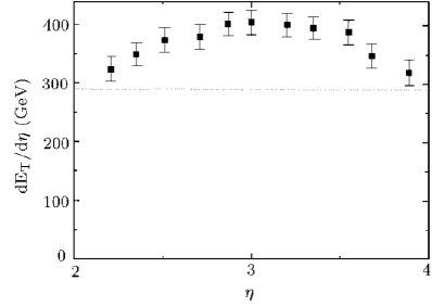
Figure 1: The Pb+Pb data of NA49. The peak is at 3.0 unit. The peak value is 405 $GeV$.

NA49 experiments showed[9] that there is a peak around $\eta=3.0$, and the peak value is 405 $GeV$ per unit. (see Fig 1.) Bjorken formula[10] gives $\epsilon_{0}=3.2$ $GeV/fm^{3}$ to fix the peak value. Setting $\epsilon_{0}=3.2$ $GeV$ and $\sigma_{0}=3.13$ $fm$ (both are near the upper limits) could also fit the peak value well, (see Fig 2,) but the peak location is $\eta=3.133$, a bit larger than expected and the peak width is only about 1 unit far smaller than the experiment. The value decrease quite rapidly far from the centre, while it is still larger than 300 $GeV$ in experiment when $\eta=2$ and 4.

Here c.m. velocities of every small regions are used instead of the particle velocities at freeze-out to compute the pseudorapidity and transverse energy. Because this method did not mention the fluid temperature and its components, one can not calculate the real momentum distribution in that small region and give the exact result. For this reason, the real curve should be more smooth and the peak should be a little lower. It means the real data are more far from the the experiment. Most of all, even if the smooth effect dominate the distribution, the total $E_{T}$ and the peak location will not change much. Counted in Fig 2, the total transverse energy between $\eta=2.0$ to 4.0, is only about 433 $GeV$, while in Fig 1, the total transverse energy is no less than 700 $GeV$. Even though set the effective size as 3.2 $fm$ to the limit, the total transverse energy is only about 464 $GeV$, while the peak value is 435.4 $GeV$ and its location comes up to 3.147 unit. Larger $\sigma_{0}$’s and initial energy densities than those are not suitable.

So one reasonable explanation is that the experimental data[9] contain a huge background[11]. This background is probably produced by the other small fireballs if multi-fireballs are emerged after the collision. The major signal from the central fireball forms the peak and the others make up a background. By cutting off the background about 290$\pm$20 $GeV$[11], the peak value decreases to about 115$\pm$20 $GeV$ and total the transverse energy turns to 123$\pm$40 $GeV$. Choosing a combination of $\sigma_{0}$ and $\epsilon_{0}$ properly, could fit it very well.

$\epsilon_{0}$ $(GeV/fm^{3})$	$1.60$	$1.80$	$2.00$	$2.20$	$2.40$
Peak value $(GeV/unit)$	$89.3$	$100.1$	$111.8$	$122.6$	$133.9$
Sum $E_{T}$ $(GeV)$	$104.0$	$117.0$	$130.0$	$143.0$	$156.0$

Table 1  Possible $\epsilon_{0}$ at $\sigma_{0}=2.5$ $fm$

$\epsilon_{0}$ $(GeV/fm^{3})$	$1.40$	$1.60$	$1.80$	$2.00$	$2.20$
Peak value $(GeV/unit)$	$90.5$	$103.1$	$116.3$	$129.0$	$142.1$
Sum $E_{T}$ $(GeV)$	$103.9$	$118.8$	$133.6$	$148.5$	$163.3$

Table 2  Possible $\epsilon_{0}$ at $\sigma_{0}=2.6$ $fm$

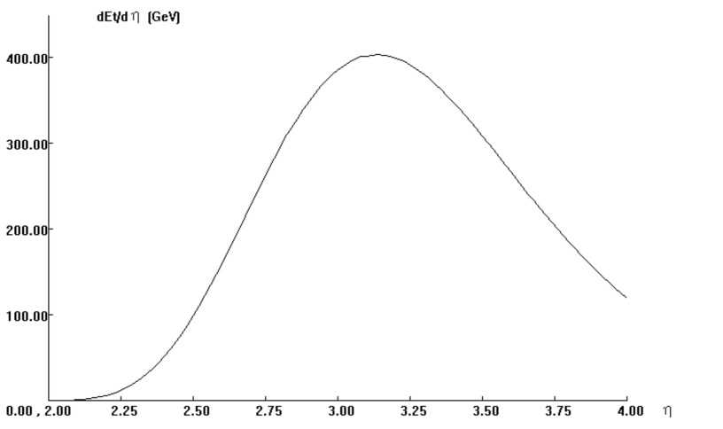
Figure 2: The $dE_{T}/d\eta$ distribution at $\epsilon_{0}=3.2$ $GeV/fm^{3}$ and $\sigma_{0}=3.13$ $fm$. The peak value is 403.9 $GeV$ and the peak location is about 3.13 unit.

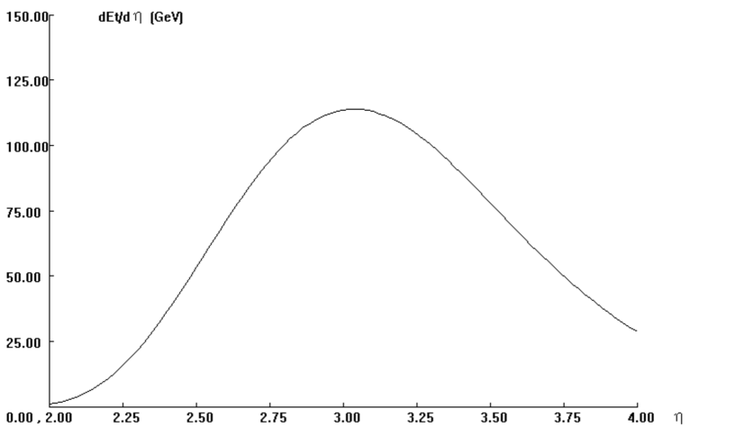
Figure 3: The $dE_{T}/d\eta$ distribution at $\epsilon_{0}=1.9$ $GeV/fm^{3}$ and $\sigma_{0}=2.55$ $fm$. The peak value is 114.0 $GeV$ and the peak location is about 3.03 unit.

Calculations show that from $\epsilon_{0}$ near 2.7 $GeV/fm^{3}$ at $\sigma_{0}=2.3$ $fm$ ($\sigma_{freeze-out}=4.300$ $fm$), $\epsilon_{0}$ near 2.0 $GeV/fm^{3}$ at $\sigma_{0}=2.5$ $fm$ ($\sigma_{freeze-out}=4.350$ $fm$) to $\epsilon_{0}$ near 1.8 $GeV/fm^{3}$ at $\sigma_{0}=2.6$ $fm$ ($\sigma_{freeze-out}=4.375$ $fm$) are all permissive. Considering that the peak location could not be too much larger or smaller than 3.0 and the transverse velocity should not be too high, $\sigma_{0}$ is defined to $[2.30,2.60]$.

The effective radius at freeze-out in experiment varies from 3.8 $fm$ by proton correlation[1][12] to $6.5\pm 0.5$ $fm$ by pion correlation[8][12]. This is quite dramatic and makes it pretty difficult to determine the initial size precisely. The effective radius got at freeze-out here varies from 4.15 $fm$ to 4.7 $fm$ according to the initial domain $\sigma_{0}=1.9\sim 3.2$ $fm$ (, see Fig 4). This result is a little larger than the the data from proton correlations and smaller than the data from pion correlations. All could be acceptable, including our conclusion $\sigma=4.3\sim 4.4$ $fm$ which is quite near to the data from proton correlations.

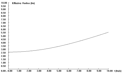
Figure 4: Fireball size during evolution. $\epsilon_{0}=$1.9 $GeV/fm^{3}$, $\sigma_{0}=$2.55 $fm$.

Transverse velocity $v_{T}$= 0.55 is reported[8][13]. Again because the local thermal momentum distribution and the particle component can not be provided from the hydronynamic method, the c.m. velocity at the effective radius $v_{\sigma}$ at freeze-out is used to compare with the transverse velocity. From $\sigma_{0}=2.3$ $fm$ to 2.6 $fm$, $v_{\sigma}$ reduces from 0.645 to 0.613. We intend to select a relatively larger initial effective radius with a lower freeze-out velocity.

Energy density at freeze-out is estimated about 0.05 $GeV/fm^{3}$[1]. Evolution results with parameters discussed above are about 0.051 to 0.065 $GeV/fm^{3}$, very approximate. Smaller and larger $\sigma_{0}$ will produce too tiny or huge result, although weone can tune the initial energy density to give a small correction.

From above, our selected estimation of the initial parameters is about $1.9\pm 0.3$ $GeV/fm^{3}$ at $\sigma_{0}=2.55$ $fm$. Detailed results are listed in Fig 5, 6, 7, 8. From Fig 5, one can see that central energy density reduces very slow (about 0.1 $GeV/fm^{3}$) in the first $1\sim 2$ $fm/c$. State that the possibilities of initial energy from range 1.4 to 2.4 $GeV/fm^{3}$ with relevant effective size could not be removed completely either.

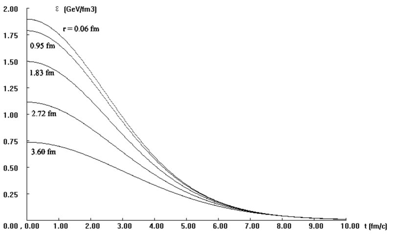
Figure 5: Energy density evolution at different locations. $\epsilon_{0}=1.9$ $GeV/fm^{3}$, $\sigma_{0}=2.55$ $fm$.

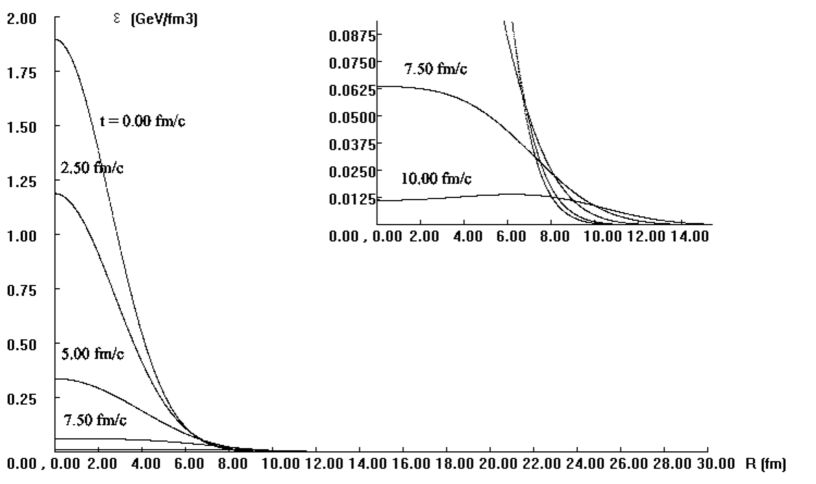
Figure 6: Energy density distributions at different time. $\epsilon_{0}=1.9$ $GeV/fm^{3}$, $\sigma_{0}=2.55$ $fm$.

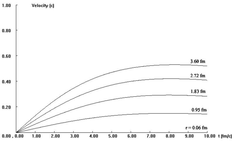
Figure 7: Fluid velocity evolution at different locations. The velocities are from a set locations, but not according to the same fluid parts. $\epsilon_{0}=1.9$ $GeV/fm^{3}$, $\sigma_{0}=2.55$ $fm$.

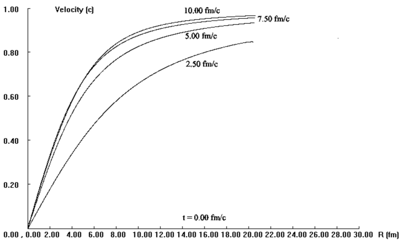
Figure 8: Fluid velocity distributions at different time. $\epsilon_{0}=1.9$ $GeV/fm^{3}$, $\sigma_{0}=2.55$ $fm$.

5. Cylindrical Fireball

In this chapter, a short discuss is done on the evolution of a flat cylindrical fireball. One more equation is added to the evolution equations (10) and one dimension of data in memory expand too. The hydrodynamic equation(s) could be written to these forms

$$\left[\frac{\partial u_{r}^{2}}{\partial r}+\frac{\partial(u_{r}u_{z})}{\partial z}+\frac{\partial(u_{r}u_{0})}{\partial t}\right]+(u_{r}^{2}+\frac{1}{4})\frac{\partial\ln\epsilon}{\partial r}+u_{r}u_{z}\frac{\partial\ln\epsilon}{\partial z}+u_{r}u_{0}\frac{\partial\ln\epsilon}{\partial t} + \frac{u_{r}^{2}}{r}=0,$$

$$\left[\frac{\partial(u_{z}u_{r})}{\partial r}+\frac{\partial u_{z}^{2}}{\partial z}+\frac{\partial(u_{z}u_{0})}{\partial t}\right]+u_{z}u_{r}\frac{\partial\ln\epsilon}{\partial r}+(u_{z}^{2}+\frac{1}{4})\frac{\partial\ln\epsilon}{\partial z}+u_{z}u_{0}\frac{\partial\ln\epsilon}{\partial t} + \frac{u_{z}u_{r}}{r}=0,$$ (14)

$$\left[\frac{\partial(u_{0}u_{r})}{\partial r}+\frac{\partial(u_{0}u_{z})}{\partial z}+\frac{\partial u_{0}^{2}}{\partial t}\right]+u_{0}u_{r}\frac{\partial\ln\epsilon}{\partial r}+u_{0}u_{z}\frac{\partial\ln\epsilon}{\partial z}+(u_{0}^{2}-\frac{1}{4})\frac{\partial\ln\epsilon}{\partial t} + \frac{u_{0}u_{r}}{r}=0.$$

Let $v_{r}=u_{r}/u_{0}$, $v_{z}=u_{z}/u_{0},$ the partial time forms

$$\frac{\partial\ln\epsilon}{\partial t} = \frac{4\alpha}{M}\left[2v_{r}A_{0}+2VzB_{0}+(\alpha-2)C_{0}\right],$$

$$\frac{\partial v_{z}}{\partial t} = -\frac{\alpha}{M}\left[2\alpha v_{z}v_{r}A_{0}+(2\alpha v_{z}^{2}+M)B_{0}+(\alpha V_{z}(\alpha-2)-Mv_{r})C_{0}\right],$$ (15)

$$\frac{\partial v_{r}}{\partial t} = -\frac{\alpha}{M}\left[2\alpha v_{r}v_{z}B_{0}+(2\alpha v_{r}^{2}+M)A_{0}+(\alpha V_{r}(\alpha-2)-Mv_{z})C_{0}\right],$$

where

$$A_{0} = \left[\frac{\partial u_{r}^{2}}{\partial r}+\frac{\partial(u_{r}u_{z})}{\partial z}+\frac{\partial(u_{r}u_{0})}{\partial t}\right]+\frac{u_{r}^{2}}{r},$$

$$B_{0} = \left[\frac{\partial(u_{z}u_{r})}{\partial r}+\frac{\partial u_{z}^{2}}{\partial z}+\frac{\partial(u_{z}u_{0})}{\partial t}\right]+\frac{u_{z}u_{r}}{r},$$

$$C_{0} = \left[\frac{\partial(u_{0}u_{r})}{\partial r}+\frac{\partial(u_{0}u_{z})}{\partial z}+\frac{\partial u_{0}^{2}}{\partial t}\right]+\frac{u_{0}u_{r}}{r},$$

and

$$\alpha = 1-v^{2}_{r}-v^{2}_{z},$$

$$M = \alpha^{2}-2\alpha+4.$$

6. Summary

Hydrodynamic equation is used to compute a spherical fireball created by the relativistic heavy ion collisions. The evolution works very well. It can produce kinds of data to compare with those from experiments. While, although these equations do not have any free parameters, but due to the complex, unknown and severe uncertain initial conditions, only a qualitative process could be given. The estimate of initial data is only a kind of attempt.

The experimental data is likely to contain a huge background. It is reported that the initial energy density could be reduced to 0.91 $GeV/fm^{3}$[11], by cutting off the background. To use hydrodynamic method to deal with this problem here, the initial energy density is estimated about $\epsilon_{0}\approx 1.9\pm 0.3$ $GeV/fm^{3}$. Thinking that the results are more sensitive to the initial size than to the initial energy density, the real error range may be larger. The result is not so striking as the estimation of $\epsilon_{0}=3.2$ $GeV/fm^{3}$ got before. The possibility of the QGP production in CERN SPS is still not clear.

Acknowledgement

We would like to thank Professor ZHUANG Pengfei for the helpful suggestions and discussions. This work was supported in part by the National Natural Science Foundation of China (90103019), and the Doctoral Programme Foundation of Institution of Higher Education, the State Education Commission of China (2000000147).

References

[1] U. W. Heinz, Nucl. Phys. A685 (2001) 414-431.
[2] J. Stachel, Nucl. Phys. A654 (1999) 119c-135c.
[3] B. Müller, Nucl. Phys. A544 (1992) 95c.
[4] P. V. Ruuskanen, Nucl. Phys. A544 (1992) 169c.
[5] U. W. Heinz, P. F. Kolb, Invited talk at the International Conference on ”Statistical QCD”.
[6] Chongshou Gao, in JingShin Theoretical Physics Symposium in Honor of Professor Ta-You Wu, edited by J. P. Hsu and L. Hsu, (World Scientific, 1998) 362.
[7] W. H. Press et al., Numerical Recipes. pp633-635. Cambridge University Press. (1986).
[8] NA49 Collaboration, Eur. Phys. J. C2 (1998) 661-670.
[9] T. Alber et al., Phys. Rev. Lett. 75 (1995) 3814.