Covariant derivative expansion of Yang-Mills effective action at high temperatures

Abstract

Integrating out fast varying quantum fluctuations about Yang–Mills fields $A_{i}$ and $A_{4}$, we arrive at the effective action for those fields at high temperatures. Assuming that the fields $A_{i}$ and $A_{4}$ are slowly varying but that the amplitude of $A_{4}$ is arbitrary, we find a nontrivial effective gauge invariant action both in the electric and magnetic sectors. Our results can be used for studying correlation functions at high temperatures beyond the dimensional reduction approximation, as well as for estimating quantum weights of classical static configurations such as dyons.

1 Introduction

The range of medium temperatures is probably one of the most interesting aspects of quantum chromodynamics (QCD). It is the region where the confinement-deconfinement phase transition is expected in the pure-glue or quenched variants of the theory, and where chiral symmetry restoration is believed to occur in the full version, with light dynamical fermions. Pure-glue theories without dynamical quarks have the advantage that one can characterize the order parameter and get insight into many interesting aspects of the phase transition [1, 2, 3, 4]. To get a good theoretical understanding of what is going on below and above the phase transitions and to understand the microscopic mechanism of the transitions themselves, is one of the greatest challenges in QCD.

Unfortunately, the present theoretical tools to handle these problems are insufficient: there are a precious few well-based statements about high and intermediate temperatures. At very high temperatures the perturbation theory in the running coupling constant can be developed. Especially the hard-thermal-loop resummation method [5] proved essential. However, perturbation theory necessarily explodes already in a few-loop approximation due to the nonperturbative chromomagnetic sector of non-Abelian gauge theories [1, 6, 7], thus limiting the applicability of perturbation theory to academically high temperatures [8]. The 1-loop [7, 9] and 2-loop [10] potential energies as functions of the ‘time’ Yang–Mills component $A_{4}$ are known, which are periodic functions with a period $2\pi T$ of the eigenvalues of $A_{4}$ in the adjoint representation. The curvature of this potential gives the Debye mass. The potential has zero-energy minima for quantized values of $A_{4}$ corresponding to the Polyakov line assuming values from the center of the gauge group. At high temperatures the system oscillates around one of those trivial values of the Polyakov line.

At lower temperatures the fluctuations in the values of the Polyakov line increase and eventually the system undergoes a transition to the phase with ${\rm Tr}\,P=0$, known as the confinement phase. To study this phase transition or at least to approach it from the high-temperature side, one needs to know the effective action for the Polyakov line in the whole range of its possible variation. Effective Lagrangians for $A_{4}$ at high temperatures have been constructed and studied by a number of authors [11, 12], however, the 1-loop kinetic energy for the Polyakov line is unknown. One of the aims of this paper is to find it.

Let us formulate the problem more mathematically. Nonzero temperatures explicitly break the $4D$ Euclidean symmetry of the theory down to the $3D$ Euclidean symmetry, so that the spatial $A_{i}$ and time $A_{4}$ components of the Yang–Mills field play different roles and should be treated differently. One can always choose a gauge where $A_{4}$ is time-independent. Taking $A_{4}(x)$ to be static is not a restriction of any kind on the fields but merely a convenient gauge choice, and we shall imply this gauge throughout the paper. [It is also a possible gauge choice at $T=0$ but in that limiting case it is unnatural as one usually wishes to preserve the $4D$ symmetry.] As to the spatial components $A_{i}(x,t)$, they are, generally speaking, timedependent, although periodic in the time direction. Putting the components $A_{i}$ to zero is a gauge noninvariant restriction on the fields since any time-independent gauge transformation will generate a nonzero $A_{i}$. Therefore, the spatial derivatives of the Polyakov line in the gauge-invariant effective action can only appear as covariant derivatives including a nonzero $A_{i}$ field.

The effective action studied in this paper is a functional of the background static $A_{4}$ field and, generally speaking, nonstatic $A_{i}$ fields, obtained by integrating out fast-varying quantum oscillations about the background. The key ingredient is that we do not assume $A_{4}$ to be small but sum up all powers in $A_{4}$. Therefore we are actually computing the effective action for the Polyakov loop interacting, in a covariant way, with the spatial $A_{i}$ fields. The resulting effective action has to be invariant with respect to time-independent gauge transformations and also with respect to certain residual timedependent gauge transformations which do not induce nonstatic $A_{4}$ and support the periodicity of $A_{i}(x,t)$; they will be discussed at the end of the paper.

An economic and æsthetic method of getting explicitly gauge invariant actions is based on the evaluation of functional determinants. [An equivalent method is computing 1-loop Feynman graphs with arbitrary number of external legs, however it is technically more involved and does not automatically support gauge invariance with respect to the external field.] In this case, the evaluation of functional determinants is nontrivial as we expand it in the (covariant) derivatives of the field but sum up all powers of the amplitude of $A_{4}$. We develop a general technique for the covariant derivative expansion which, in principle, can be worked out to any power of the derivatives. In this paper, however, we find explicit expressions for the action with 0,2 and 4 covariant derivatives. This enables us to find the leading terms both in the electric and magnetic sectors of the theory.

Since $4D$ Euclidean invariance is broken by nonzero temperature the electric and magnetic field strengths appear differently in the action. The magnetic field strength is

$$B^{a}_{i}=\frac{1}{2}\epsilon_{ijk}\left(\partial_{j}A_{k}^{a}-\partial_{k}A_{j}^{a}+\epsilon^{abc}A_{j}^{b}A_{k}^{c}\right),$$ (1)

whereas the electric field strength consists of two pieces, the ‘static’ and the ‘dynamical’:

$$E_{i}^{a}=D_{i}^{ab}A_{4}^{b}-\dot{A}_{i}^{a}=\partial_{i}A_{4}^{a}+\epsilon^{acb}A_{i}^{c}A_{4}^{b}-\dot{A}_{i}^{a}.$$ (2)

In the $SU(2)$ gauge theory to which we mostly restrict ourselves in the present paper there are only a few gauge and Euclidean $3D$ invariants in the order we are interested in. These are $A_{4}^{a}A_{4}^{a}$, $E_{i}^{a}E_{i}^{a}$, $B_{i}^{a}B_{i}^{a}$ and $(E_{i}^{a}A_{4}^{a})^{2}$, $(B_{i}^{a}A_{4}^{a})^{2}$. [For higher gauge groups there will be more invariants.] The effective action (tree plus 1-loop) has the form

$$S_{\rm eff}\!\! = \!\int\frac{d^{3}x}{T}\left[-T^{4}V(\nu)\!+\!E_{i}^{2}F_{1}(\nu)\!+\!\frac{(E_{i}A_{4})^{2}}{A_{4}^{2}}F_{2}(\nu)\!\right.+\left.\!B_{i}^{2}\,H_{1}(\nu)\!+\!\frac{(B_{i}A_{4})^{2}}{A_{4}^{2}}\,H_{2}(\nu)\!+\!\ldots\!\right]\,,$$ (3)

$$\nu = \frac{\sqrt{A_{4}^{a}A_{4}^{a}}}{2\pi T}.$$

The static potential $V(\nu)$ has been known for 20 years [7, 9]; the functions $F_{1,2},\,H_{1,2}$ are the new findings of this paper: they turn out to be quite nontrivial and can be expressed through the digamma $\psi$ functions. The $E_{i}^{2}A_{4}^{2}$ and $B_{i}^{2}A_{4}^{2}$ terms of the effective action (corresponding to the first terms of the Taylor expansion of our functions) have been known before [13] and one combination (actually $F_{1}+F_{2}$ in our notations) was actually found previously by considering a particular case of $A_{i}=0$ [14]. We agree with this previous work, however our results are, of course, more general. In addition to the structures in eq. (3) we have found a full-derivative term in the effective action. This term is not necessarily zero: if the background field does not fall off fast enough at spatial infinity it gives a finite contribution. This is, e.g., the case when the background field is that of the BPS dyon [15].

Actually, quantum determinants are UV divergent, giving rise to the renormalization of the bare coupling constant of the tree action. We perform an accurate regularization of the determinants by means of the Pauli–Villars scheme. As a result, the above functions are finite and the $F_{1},\,H_{1}$ functions contain the running-coupling terms $\frac{11}{24\pi^{2}}\,\ln\left(\frac{T}{\Lambda}\,{\rm const.}\right)$ where $\Lambda$ is the QCD scale in a particular regularization scheme. We have determined the value of the ‘const.’ in the argument of the logarithm and hence have learned the precise scale of the running coupling constant at which it needs to be evaluated. Changing the regularization scheme means the substitution $\Lambda_{\rm PV}=e^{\frac{1}{22}}\Lambda_{\overline{\rm MS}}=40.66\cdot\textnormal{exp}\left(-\frac{3\pi^{2}}{11N^{2}}\right)\,\Lambda_{\rm Lat}=\ldots$ [16].

There are two different approaches to the effective action and correspondingly two different variants of the resulting functions $F_{1,2}...$ One can either exclude or include the contribution of the static (zero Matsubara frequency) fluctuations to the effective action. One follows the former logic if one wishes to get the effective action for static modes only. In this case the potential energy $V(A_{4})$ is not periodic and moreover it is formally UV divergent. One follows the latter logic if one is interested, e.g., in finding full quantum corrections to semiclassical field configurations at nonzero temperatures, the examples of such being dyons [17] and calorons [18]. We compute the functions $F_{1,2}$ and $H_{1,2}$ in both variants.

Correspondingly, we think of two kinds of applications of our results. One is for studying the fluctuations and correlation functions of the Polyakov line in the region of temperatures where its average deviates considerably from the perturbative center-of-group values and where the dimensional reduction (i.e. perturbative) approximation fails. Another application is for evaluating the weights of semiclassical objects appearing at nonzero temperature [19].

2 Basics of Yang-Mills theory at finite temperature

The general definition of the partition function for statistical systems is

$${\cal Z} = \sum_{n}\langle n\left|e^{-\beta{\cal H}}\right|n\rangle\qquad\quad{\left[\beta=\frac{1}{T}\right]}$$ (4)

$$= \sum_{n}\int\!dq\,\psi^{*}_{n}(q)\;e^{-\beta{\cal E}_{n}}\;\psi_{n}(q)=\int\!dq_{0}\int_{q(0)=q_{0}}^{q(\beta)=q_{0}}Dq(t)\,\textnormal{exp}\left(-\int_{o}^{\beta}\!dt{\cal H}[q,\dot{q}]\right)\,,$$ (5)

where ${\cal H}$ is the Hamiltonian of the system, and ${\cal E}_{n}$ are its eigenvalues. In Yang-Mills theory the role of coordinates $q$ is played by the amplitudes of the gluon fields $A_{i}^{a}(x)$ and the Hamiltonian is

$$\beta{\cal H}=\frac{1}{2g^{2}}\int_{0}^{\beta}\!dx_{4}\!\int\!d^{3}x\left[\left(\dot{A}_{i}^{a}\right)^{2}+\left(B_{i}^{a}\right)^{2}\right]\,,$$ (6)

where the dot indicates time derivative and $B_{i}^{a}$ is the magnetic field (1). The partition function can be written as a path integral over ‘trajectories’ $A_{i}(x_{4},x)$ going from a ‘coordinate’ $A_{i}^{(0)}$ at $x_{4}=0$ to the same coordinate at $x_{4}=\beta$; one also has to integrate over this initial coordinate:

$${\cal Z}=\int DA_{i}^{(0)}(x)\int_{A_{i}(0,x)=A_{i}^{(0)}}^{A_{i}(\beta,x)=A_{i}^{(0)}}DA_{i}(x_{4},x)\,\textnormal{exp}\left\{-\frac{1}{2g^{2}}\,\int_{0}^{\beta}\!dx_{4}\,\int\,d^{3}x\left[\left(\dot{A}_{i}^{a}\right)^{2}+\left(B_{i}^{a}\right)^{2}\right]\right\}\;.$$ (7)

However, in a gauge theory one sums not over all possible but only over physical states, i.e. satisfying Gauss’ law. In the absence of external sources it means that only those states need to be taken into account that are invariant under gauge transformations:

$$A_{i}(x)\to\left[A_{i}(x)\right]^{\Omega(x)} = \Omega(x)^{\dagger}\,A_{i}(x)\,\Omega(x)+i\Omega(x)^{\dagger}\,\partial_{i}\Omega(x),$$ (8)

$$\qquad\Omega(x) = \textnormal{exp}\{i\,\omega_{a}(x)t^{a}\}\;.$$

To restrict the summation to physical states, one has to modify eq. (7). One projects to the physical i.e. gauge invariant states by averaging the initial and final configurations over gauge rotations. The YM partition function is therefore

$${\cal Z_{\rm phys}}\!\!\! = \!\!\sum_{\rm phys\;states}\langle n\left|e^{-\beta{\cal H}}\right|n\rangle$$ (9)

$$= \!\!\!\!\!\!\!\int\!\!\!D\Omega_{1,2}(x)D\!A_{i}^{(0)}(x)\!\!\!\int_{A_{i}(0,x)=[A_{i}^{(0)}]^{\Omega_{1}(x)}}^{A_{i}(\beta,x)=[A_{i}^{(0)}]^{\Omega_{2}(x)}}\!\!\!\!D\!A_{i}(x_{4},x)\,\textnormal{exp}\!\left\{\!\!-\frac{1}{2g^{2}}\!\!\int_{0}^{\beta}\!\!\!dx_{4}\!\!\int\!\!\!d^{3}x\!\!\left[\!\left(\!\dot{A}_{i}^{a}\!\right)^{2}\!\!\!+\!\!\left(B_{i}^{a}\right)^{2}\right]\!\right\}\!.$$

Renaming the initial field $[A_{i}^{(0)}]^{\Omega_{1}(x)}\to A_{i}^{(0)}$ and introducing the relative gauge transformation $\Omega(x)=\Omega_{2}(x)\,\Omega_{1}^{\dagger}(x)$ one can rewrite this as [7]

$${\cal Z_{\rm{phys}}}=\,\int\,D\Omega(x)DA_{i}^{(0)}(x)\int_{A_{i}^{(0)}}^{[A_{i}^{(0)}]^{\Omega(x)}}\,DA_{i}(x_{4},x)\;e^{-\beta{\cal H}[A_{i}(x_{4},x)]}\;.$$ (10)

There is a subtle question whether one has to include integration over global gauge transformations, i.e. $x$-independent $\Omega$’s in eq. (10). If one does, it means that only states with total color charge zero are admitted in the partition function. A more cautious approach is to allow for states with nonzero color charge: if these are for some reasons dynamically suppressed it must be seen from the theory but not imposed by hand. Therefore we shall admit x-independent $\Omega$’s but not integrate over them explicitly.

In order to put the partition function into a more customary four dimensional form one introduces an interpolating gauge transformation $\Omega(x_{4},x)$ such that

$$\Omega(x_{4},x) = \left\{\begin{array}[]{cc}{\bf 1},&x_{4}=0,\\ \Omega(x),&x_{4}=\beta\end{array}\right.\;.$$ (13)

Simultaneously one changes the integration variables from $A_{i}(x_{4},x)$ to

$$A_{i}^{\prime}(x_{4},x)=\Omega(x_{4},x)\,A_{i}(x_{4},x)\Omega^{\dagger}(x_{4},x)+i\Omega(x_{4},x)\,\partial_{i}\,\Omega^{\dagger}(x_{4},x)$$ (14)

and introduces, instead of $\Omega(x_{4},x)$, the new variable

$$A_{4}(x_{4},x)=i\Omega(x_{4},x)\,\partial_{4}\,\Omega^{\dagger}(x_{4},x).$$ (15)

For example, if the interpolating gauge transformation is taken to be $\Omega(x_{4},x)=\textnormal{exp}\{i\,x_{4}\,T\,\omega^{a}(x)\,t^{a}\}$, then $A_{4}$ is time-independent and equal to $A_{4}(x)=T\,\omega^{a}(x)\,t^{a}$. We note that both $A_{4}(x_{4},x)$ and $A_{i}^{\prime}(x_{4},x)$ are periodic in temporal direction.

The magnetic energy is gauge invariant, i.e.

$${\rm Tr}\,B^{2}(A_{i})={\rm Tr}\,B^{2}(A_{i}^{\prime})\;,$$ (16)

while the electric energy becomes

$${\rm Tr}\,E^{2}={\rm Tr}\,\dot{A}_{i}^{2}={\rm Tr}\,{E^{\prime}}^{2}\;,$$ (17)

where

$$E_{i}^{\prime}=\dot{A}_{i}^{\prime}-\partial_{i}\,A_{4}-i\,[A_{4},A_{i}^{\prime}]=\dot{A}_{i}^{\prime}-[\nabla_{i}(A^{\prime})A_{4}].$$ (18)

Therefore the full action density can be rewritten as a standard ${\rm Tr}\,F_{\mu\nu}^{2}$, where

$$F_{\mu\nu}=\partial_{\mu}A_{\nu}-\partial_{\nu}A_{\mu}-i\,[A_{\mu},A_{\nu}]$$ (19)

with $A_{\mu}(x_{4},x)$ denoting $A_{i}^{\prime}(x_{4},x)$ and $A_{4}(x_{4},x)$. Thus, eq. (10) is equivalent to the more familiar partition function

$${\cal Z}_{\rm phys}=\int DA_{\mu}\,\textnormal{exp}\left\{-\frac{1}{4g^{2}}\int\!d^{4}x\,F_{\mu\nu}^{a}F_{\mu\nu}^{a}\right\},$$ (20)

where one integrates over gauge fields obeying periodic boundary conditions in time, meaning $A_{\mu}(x_{4},x)=A_{\mu}(x_{4}+\beta,x)$, with $\beta=1/T$.

Periodic fields can be decomposed into Fourier modes:

$$A_{\mu}(x_{4},x)=\sum_{k=-\infty}^{\infty}A(\omega_{k},x)\,e^{i\omega_{k}x_{4}},\qquad{\omega_{k}=2\pi k\,T.}\;$$ (21)

where $\omega_{k}=2\pi k\,T$ are the so-called Matsubara frequencies, which play the role of mass. In the limit $T\to\infty$ all nonzero Matsubara modes become infinitely heavy. If one leaves only the static gluon modes it is called dimensional reduction [20], as the resulting theory is purely static. There is no dynamics in the time direction anymore. At high, but not infinite temperatures, this approximation is too crude. The nonzero modes show up in loops and produce infinitely many effective vertices. The aim of this paper is to find all these infinite number of vertices restricted, however, to low momenta $p<T$, induced in the 1-loop order.

3 One loop quantum action

As stressed in the Introduction, one can always choose the background field $A_{4}$ to be static. As to the $A_{i}$ field, we shall temporarily take it to be static: the generalization of the effective action to the case of timedependent $A_{i}$ will be simple.

To study the effects of the nonzero Matsubara modes we use a background field method and split the gluon fields into a time independent background field $\bar{A}_{\mu}(x)$ and a presumably small quantum fluctuation field $a_{\mu}(x_{4},x)$:

$$A_{\mu}(x_{4},x)=\bar{A}_{\mu}(x)+a_{\mu}(x_{4},x)\;.$$ (22)

In this paper we consider the quantum effects at the 1-loop level. Then it is sufficient to expand the action around the background field up to quadratic order in $a_{\mu}$. The linear term in $a_{\mu}$ is absent owing to the orthogonality of nonstatic modes to static ones. We shall, however, also investigate the contribution of the static fluctuation mode. In this case the linear term is absent if, e.g., the background field satisfies the equation of motion or if the static mode is varying in space faster than the background field. The quadratic form is, generally speaking, degenerate so that one has to fix the gauge for fluctuations. This gauge fixing is unrelated to the gauge fixing of the background field. We choose the background Lorenz gauge $D_{\mu}(\bar{A})a_{\mu}=0$ , where

$$D_{\mu}^{ab}(\bar{A})=\partial_{\mu}\delta^{ab}+f^{acb}\bar{A}_{\mu}^{c}\;.$$ (23)

is the covariant derivative in the adjoint representation. This gauge brings in the Faddeev-Popov ghost determinant which can be expressed as a Grassmann integral over ghost fields. For the partition function this yields

$$Z(\bar{A})=e^{S}=e^{\bar{S}}\,\int{}Da\,D\chi\,D\chi^{+}\,\textnormal{exp}\left\{-\frac{1}{2g^{2}(M)}\int{}d^{4}x\,a_{\mu}^{b}\,W_{\mu\nu}^{bc}\,a_{\nu}^{c}-\int\,d^{4}x\,\chi^{+a}\left(D^{2}_{\mu}\right)\,\chi^{a}\right\}\;,$$ (24)

where $\chi,\chi^{+}$ are ghost fields and

$$\bar{S}=-\frac{1}{4g^{2}(M)}\int\,d^{4}x{}F_{\mu\nu}^{a}(\bar{A})F_{\mu\nu}^{a}(\bar{A})$$ (25)

is the action of the background field. The quadratic form for $a_{\mu}$ in the background Lorenz gauge is given by

$$W_{\mu\nu}^{ab}=-[D^{2}(\bar{A})]^{ab}\delta_{\mu\nu}-2f^{acb}F_{\mu\nu}^{c}(\bar{A})\;.$$ (26)

Integrating out the quantum fluctuations and ghosts yields two functional determinants,

$$Z(\bar{A})=e^{\bar{S}}\;\left(\textnormal{det}{W}\right)^{-1/2}\;\textnormal{det}\left(-D^{2}\right)\;,$$ (27)

so that the 1-loop action is

$$S_{\rm{1-loop}}=\textnormal{log}\,\left(\textnormal{det}{W}\right)^{-1/2}+\textnormal{log}\,\textnormal{det}\left(-D^{2}\right)\;.$$ (28)

Since the operators $D^{2},W_{\mu\nu}$ are built from covariant derivatives and the field strength only, this action is invariant under general gauge transformations of the background field. One can use this freedom to make the $A_{4}$ component static, which we shall always assume. The spatial components $A_{i}$ are then, generally speaking, time dependent. For the most of the paper we shall assume that $A_{i}$ is time-independent too. At the end we shall be able to reconstruct terms with $\dot{A}_{i}$ from gauge invariance but at the time being we shall take static $A_{i}$. Then the quantum action (28) is invariant under time-independent gauge transformations,

$$\bar{A_{4}}(x) \to U(x)\,\bar{A_{4}}(x)\,U^{\dagger}(x),$$ (29)

$$\bar{A_{i}}(x) \to U(x)\,\bar{A_{i}}(x)\,U^{\dagger}(x)+i\,U(x)\,\partial_{i}\,U^{\dagger}(x)\;.$$ (30)

In this paper we restrict ourselves to the $SU(2)$ color group, which means that the action depends on the gauge and $3D$ Euclidean invariants $A_{4}^{a}A_{4}^{a}$, $E_{i}^{a}E_{i}^{a}$, $B_{i}^{a}B_{i}^{a}$, $E_{i}^{a}A_{4}^{a}$, $B_{i}^{a}A_{4}^{a}$, etc. For higher groups there will be more invariants. We write the background fields without a bar from now on, as they are the only field variables left.

In fact the action can be presented as a series in the spatial covariant derivative $D_{i}$. Since the electric field is given by $E_{i}^{a}=D_{i}^{ab}A_{4}^{b}$, an expansion in powers of the electric field corresponds to a covariant gradient expansion of the $A_{4}$ fields. To get the magnetic field, we already need one more power of $D_{i}$, as $B_{k}^{a}=\frac{1}{2}\epsilon_{ijk}F_{ij}^{a}=\frac{1}{4}\epsilon_{ijk}\epsilon^{cad}\left[D_{i},D_{j}\right]^{cd}$. For the $SU(2)$ gauge group, in the electric (magnetic) sector only two independent color vectors exist, $E_{i}^{a}$ ($B_{i}^{a}$) and $A_{4}^{a}$. Therefore, we expect the following structure for the gauge-invariant gradient expansion:

$$S_{\rm{1-loop}}\!\!=\!\int\frac{d^{3}x}{T}\left[-T^{4}\,V(\nu)\!+\!E_{i}^{2}f_{1}(\nu)\!+\!\frac{(E_{i}A_{4})^{2}}{A_{4}^{2}}f_{2}(\nu)\!+\!B_{i}^{2}\,h_{1}(\nu)\!+\!\frac{(B_{i}A_{4})^{2}}{A_{4}^{2}}\,h_{2}(\nu)\!+\!\ldots\!\right].$$ (31)

In the explicit evaluation of the functional determinants we find exactly the structure eq. (31) and determine the functions $f_{1},f_{2},h_{1},h_{2}$ at all values of their argument which is in fact a dimensionless ratio $\nu=\sqrt{A_{4}^{a}A_{4}^{a}}/(2\pi T)$.

4 The functional determinants

We start with the evaluation of the ghost functional determinant. As usual we subtract the zero gluon field contribution. Using the fact that $\textnormal{det}\,{\rm K}=\textnormal{exp}\,{\rm Tr}\,\textnormal{log}\,{\rm K}$ we can write

$$\textnormal{exp}\,\textnormal{log}\,\frac{\textnormal{det}(-D_{\mu}^{2})}{\textnormal{det}(-\partial_{\mu}^{2})}=\textnormal{exp}\;{\rm Sp}\,[\textnormal{log}\,(-D_{\mu}^{2})-\textnormal{log}\,(-\partial_{\mu}^{2})]$$ (32)

where ${\rm Sp}$ is a functional trace. We present the ratio of determinants with the help of the Schwinger proper time representation [22]:

$$\textnormal{log}\,\textnormal{det}(-D^{2})_{\rm{n}}\equiv\textnormal{log}\,\frac{\textnormal{det}(-D_{\mu}^{2})}{\textnormal{det}(-\partial_{\mu}^{2})}=-\int_{0}^{\infty}\frac{ds}{s}\;{\rm Sp}\left(e^{sD_{\mu}^{2}}-e^{s\partial_{\mu}^{2}}\right)\;.$$ (33)

In fact this ratio is logarithmically UV divergent, reflecting the coupling constant renormalization. We use the Pauli-Villars method to regularize the divergence. This corresponds to replacing the determinant by a ‘quadrupole formula’:

$$\textnormal{det}(-D^{2})\longrightarrow\textnormal{det}(-D^{2})_{\rm{r,n}}$$ (34)

$$\equiv\frac{\textnormal{det}(-D_{\mu}^{2})}{\textnormal{det}(-\partial_{\mu}^{2})}\,\frac{\textnormal{det}(-\partial_{\mu}^{2}+M^{2})}{\textnormal{det}(-D_{\mu}^{2}+M^{2})} = \textnormal{exp}\left\{-\int_{0}^{\infty}\frac{ds}{s}\;{\rm Sp}\left[\left(1-e^{-sM^{2}}\right)\,\left(e^{sD_{\mu}^{2}}-e^{s\partial_{\mu}^{2}}\right)\right]\right\}\;.$$ (35)

The functional trace in eq. (35) can be taken by inserting any full basis, so we are free to choose e.g. the plane-wave basis, $\textnormal{exp}(ix_{\alpha}p_{\alpha})$. Then, by the definition of the functional trace, one can write

$${\rm Sp}\,e^{-sK}={\rm Tr}\,\int\,d^{4}x\,\lim_{y\to x}\int\frac{d^{4}p}{(2\pi)^{4}}\,\textnormal{exp}(-ip\cdot y)\textnormal{exp}(-sK)\,\textnormal{exp}(ip\cdot x),$$ (36)

where ${\rm Tr}$ is the remaining matrix trace over color and, as the case may be, Lorentz indices. One can now drag the latter plane-wave exponent though the differential operator $K$ until it cancels with the former. This results in the shift of the derivatives inside the differential operator and in the following representation of the functional trace [23]:

$${\rm Sp}\,e^{-sK}={\rm Tr}\,\int\,d^{4}x\,\int\frac{d^{4}p}{(2\pi)^{4}}\,\textnormal{exp}\left[-sK(\partial_{\alpha}\rightarrow\partial_{\alpha}+ip_{\alpha})\right]\bf{1}\,.$$ (37)

The $\bf{1}$ at the end is meant to emphasize that the shifted operator acts on unity, so that for example any term that has a $\partial_{\alpha}$ in the exponent and is brought all the way to the right, will vanish. According to (37) we now have

$$\textnormal{log}\,\textnormal{det}(-D^{2})_{\rm{r,n}}=-\int\,\frac{d^{3}x}{T}\,T\sum_{k=-\infty}^{\infty}\int\frac{d^{3}p}{(2\pi)^{3}}\,\int_{0}^{\infty}\frac{ds}{s}\left(1-e^{-sM^{2}}\right)$$ (38)

$$\times {\rm Tr}\,\left\{\textnormal{exp}\left[s(D_{4}+i\omega_{k})^{2}+s(D_{i}+ip_{i})^{2}\right]-\textnormal{exp}\left[s(i\omega_{k})^{2}+s(ip_{i})^{2}\right]\right\}\;.$$ (39)

Owing to the periodic boundary conditions we have replaced the integration over $p_{4}$ by the sum over the Matsubara frequencies $\omega_{k}=2\pi kT$ and taken into account that the $x_{4}$ integration goes from $0$ to $\beta=1/T$. Keeping in mind that the background field is time independent one can replace

$$D_{4}^{ab}\to f^{acb}A_{4}^{c}\;.$$ (40)

We define the adjoint matrix

$$\mathcal{A}^{ab}=f^{acb}A_{4}^{c}+i\omega_{k}\delta^{ab}$$ (41)

upon which eq. (38) becomes

$$\textnormal{log}\,\textnormal{det}(-D^{2})_{\rm{r,n}}=-\int\,d^{3}x\,\sum_{k=-\infty}^{\infty}\int\frac{d^{3}p}{(2\pi)^{3}}\,\int_{0}^{\infty}\frac{ds}{s}\,\left(1-e^{-sM^{2}}\right)$$ (42)

$$\times {\rm Tr}\,\left\{\textnormal{exp}\left[s\mathcal{A}^{2}+sD_{i}^{2}+2isp_{i}D_{i}-sp^{2}\right]-\textnormal{exp}\left[-s(\omega_{k}^{2}+p^{2})\right]\right\}\;.$$ (43)

In the same way as for the ghost determinant (32) we use the ‘quadrupole formula’ and write the normalized and regularized gluon determinant as

$$\textnormal{log}\,(\textnormal{det}W)^{-1/2}_{{\rm r,n}}=\frac{1}{2}\,\int_{0}^{\infty}\frac{ds}{s}\left(1-e^{-sM^{2}}\right){\rm Sp}\left(e^{-sW_{\mu\nu}^{ab}}-e^{s\partial^{2}\,\delta_{\mu\nu}\delta^{ab}}\right)\;,$$ (44)

which after an insertion of a plane wave basis and dragging $\textnormal{exp}(ip\cdot x)$ through the differential operator yields

$$\textnormal{log}\,(\textnormal{det}W)^{-1/2}_{{\rm r,n}}=\frac{1}{2}\int\,d^{3}x\,\sum_{k=-\infty}^{\infty}\int\frac{d^{3}p}{(2\pi)^{3}}\,\int_{0}^{\infty}\frac{ds}{s}\left(1-e^{-sM^{2}}\right)$$

$$\times {\rm Tr}\,\left\{\textnormal{exp}\left[(s\mathcal{A}^{2}+sD_{i}^{2}+2isp_{i}D_{i}-sp^{2})^{ab}\delta_{\mu\nu}+2sf^{acb}F_{\mu\nu}^{c}\right]-\textnormal{exp}\left[-s(\omega_{k}^{2}+p^{2})\right]\right\}\;.$$

A covariant gradient or derivative expansion is the expansion in $D_{i}$, applied to $\mathcal{A}^{2}$ and $F_{\mu\nu}^{c}$. For example, to quadratic order in $D_{i}$ it corresponds to summing up all 1-loop Feynman diagrams with two $A_{4}$ vertices carrying momenta, and any number of $A_{4}$ insertions at zero momentum. So far, both eq. (42) and eq. (4) are independent of the gauge group.

5 Zeroth order of covariant derivative expansion

Zeroth order in the expansion corresponds to setting $D_{i}=0$. For the gluon part (4) the field strength does not contribute at this order since it is quadratic in the covariant derivatives. Hence the gluonic contribution is $-(1/2)\times 4=-2$ times the ghost contribution, where the factor $(-1/2)$ comes from the fact that the gluon determinant is taken to this power (see (27)), and the Lorentz structure of the gluons, ${\rm Tr}\,\delta_{\mu\nu}$, yields 4. At zeroth order of the covariant derivative expansion one thus has:

$$S_{\rm{1-loop}}^{(0)}=-\left[\textnormal{log}\,\textnormal{det}\left(-D^{2}\right)\right]^{(0)}\;.$$ (46)

The determinant is UV finite in this order, so one does not need to regularize it. For the explicit calculation one can choose a gauge where $A_{4}$ is diagonal in the fundamental representation, hence for the $SU(2)$ gauge group

$$A_{4}^{a}=\delta^{a3}\phi\qquad,\qquad\phi=\sqrt{A_{4}^{a}\,A_{4}^{a}}\;.$$ (47)

The eigenvalues of the $3\times 3$ matrix $\mathcal{A}^{ab}=\epsilon^{a3b}\phi+i\omega_{k}\delta^{ab}$ are $\left(\omega_{k}+\phi,\omega_{k}-\phi,\omega_{k}\right)$. It is obvious that upon summation over all Matsubara frequencies $f[(\omega_{k}+\phi)^{2}]$ and $f[(\omega_{k}-\phi)^{2}]$ give the same. We hence obtain

$$S_{\rm{1-loop}}^{(0)}=2\int\,d^{3}x\,\sum_{k=-\infty}^{\infty}\int\frac{d^{3}p}{(2\pi)^{3}}\,\int_{0}^{\infty}\,\frac{ds}{s}\,e^{-sp^{2}}\left\{e^{-s(\omega_{k}-\phi)^{2}}-e^{-s\omega_{k}^{2}}\right\}\;.$$ (48)

Integrating over proper time $s$ and summing over Matsubara frequencies labeled by $k$ gives

$$\sum_{k=-\infty}^{\infty}\int_{0}^{\infty}\,\frac{ds}{s}\,e^{-s(\omega_{k}-\phi)^{2}-sp^{2}}=-\textnormal{log}\left({\rm ch}\frac{|\vec{p}|}{T}-{\rm cos}\frac{\phi}{T}\right)\;.$$ (49)

The $p$ integration can be performed with the help of Ref. [24]. One obtains

$$S_{\rm{1-loop}}^{(0)}=-\int d^{3}x\frac{1}{12\pi^{2}T}\phi^{2}\left(2\pi T-\phi\right)^{2}{|}_{{\rm mod}\;2\pi T}\;,$$ (50)

hence the dimensionless static potential is

$$V(\nu)=\frac{(2\pi)^{2}}{3}\,\nu^{2}\,(1-\nu)^{2}{|}_{{\rm mod}\;1},\qquad\nu=\frac{\sqrt{A_{4}^{a}A_{4}^{a}}}{2\pi T}\,.$$ (51)

This result is well known [7, 9]. We want to stress here that the term cubic in $\nu$ arises solely from the zero Matsubara frequency, $k=0$. It makes eq. (50) periodic in $\nu$ with unit period. It should be noted that without the zero frequency contribution the $p$ integration is UV divergent; the addition of the $\omega_{k}=0$ mode removes this divergence.

6 General technique for the covariant derivative expansion

In the next orders in the covariant derivative the calculation becomes more involved. We wish to keep all powers of $A_{4}$, but expand in powers of $D_{i}$. To expand the exponential of two noncommuting operators A and B we use the formulae

$$e^{A+B}=e^{A}+\int_{0}^{1}\,d\alpha\,e^{\alpha A}Be^{(1-\alpha)A}+\int_{0}^{1}\,d\alpha\,\int_{0}^{1-\alpha}\,d\beta\,e^{\alpha A}B\,e^{\beta A}Be^{(1-\alpha-\beta)}A+\ldots\;$$ (52)

and

$$\left[B,e^{A}\right]=\int_{0}^{1}d\gamma\,e^{\gamma A}\left[B,A\right]\,e^{(1-\gamma)A}\;.$$ (53)

Here $B$ denotes the combination of covariant derivatives in the exponents in eq. (42) or eq. (4), $A$ is everything that is left there. We encounter here the following commutators:

$$\left[D_{i},\mathcal{A}\right] = \left[D_{i},D_{4}\right]=-i\,F_{i4}=-iE_{i}\;,$$ (54)

$$\left[D_{i},\mathcal{A}^{2}\right] = -i\left\{\mathcal{A},E_{i}\right\}\;,$$ (55)

where the electric field is in the adjoint representation, i.e.

$$E_{i}^{ab}=if^{acb}E_{i}^{c}\;.$$ (56)

The strategy is to drag all derivatives in $B$ to the right using the master formulae (52,53).

7 Electric sector

We are now going to find the second and third terms in eq. (31), i.e. terms quadratic in the covariant derivative $D_{i}$. As expected, terms which are not gauge invariant cancel out individually for the ghosts and the gluons. In the end three different gauge invariant contributions remain. Writing down the ghost determinant as

$$\textnormal{log}\,\textnormal{det}(-D^{2})_{\rm{r,n}}=-\int\,d^{3}x\,\sum_{k=-\infty}^{\infty}\int\frac{d^{3}p}{(2\pi)^{3}}\,\int_{0}^{\infty}\frac{ds}{s}\left(1-e^{-sM^{2}}\right){\rm Tr}\,e^{-sp^{2}}\left[e^{A+B}\right]\;,$$ (57)

where $A=s\mathcal{A}^{2}$ and $B=2isp_{i}D_{i}+sD_{i}^{2}$ and expanding in $B$ with the use of eqs. (52,53) we obtain [see Appendix B.1]

$$\left[\textnormal{log}\,\textnormal{det}(-D^{2})_{{\rm r,n}}\right]_{{\rm E}}^{(2)}=-\int\,d^{3}x\,\sum_{k=-\infty}^{\infty}\int\frac{d^{3}p}{(2\pi)^{3}}\,\int_{0}^{\infty}\frac{ds}{s}\left(1-e^{-sM^{2}}\right)\,e^{-sp^{2}}\left[I_{1}+I_{2}\right]\;.$$ (58)

The gluon determinant is

$$\textnormal{log}\,(\textnormal{det}W)^{-1/2}_{{\rm r,n}}=\frac{1}{2}\int\,d^{3}x\,\sum_{k=-\infty}^{\infty}\int\frac{d^{3}p}{(2\pi)^{3}}\,\int_{0}^{\infty}\frac{ds}{s}\left(1-e^{-sM^{2}}\right){\rm Tr}\,e^{-sp^{2}\delta_{\mu\nu}}\left[e^{A+B}\right]\;,$$ (59)

where this time $A_{\mu\nu}^{ab}=(s\mathcal{A}^{2})^{ab}\,\delta_{\mu\nu}$ and $B_{\mu\nu}^{ab}=(sD_{i}^{2}+2isp_{i}D_{i})^{ab}\delta_{\mu\nu}+2sf^{acb}F_{\mu\nu}^{c}$. Expanding in $B_{\mu\nu}^{ab}$ and using eqs. (52,53) we find [see Appendix B.1]

$$\left[\textnormal{log}\,(\textnormal{det}W)^{-1/2}_{{\rm r,n}}\right]_{{\rm E}}^{(2)}=\int\,d^{3}x\,\sum_{k=-\infty}^{\infty}\int\frac{d^{3}p}{(2\pi)^{3}}\,\int_{0}^{\infty}\frac{ds}{s}\left(1-e^{-sM^{2}}\right)\,e^{-sp^{2}}\left[2I_{1}+2I_{2}+\frac{I_{3}}{2}\right]\;.$$ (60)

The gauge invariants in eqs. (58,60) are

$$I_{1} = \!\!s^{3}\!\int_{0}^{1}\!d\alpha\!\left\{\!-\frac{1}{2}+\alpha(1\!-\!\alpha)+\frac{2}{9}sp^{2}\left[1\!-\!\frac{3}{2}\alpha(1\!-\!\alpha)\right]\!\right\}\!\!{\rm Tr}\,e^{(1-\alpha)s\mathcal{A}^{2}}\!\left\{\mathcal{A},E_{i}\right\}\!e^{\alpha s\mathcal{A}^{2}}\!\!\left\{\mathcal{A},E_{i}\right\}\!,$$ (61)

$$I_{2} = \!\!-s^{2}\left(\frac{1}{2}-\frac{2}{9}sp^{2}\right)\,{\rm Tr}\,e^{s\mathcal{A}^{2}}\left(2E_{i}^{2}+i\left\{\mathcal{A},\left[D_{i},E_{i}\right]\right\}\right),$$ (62)

$$I_{3} = \!\!8s^{2}\int_{0}^{1}\,d\alpha\,\frac{1}{2}\,{\rm Tr}\,e^{(1-\alpha)s\mathcal{A}^{2}}\,E_{i}\,e^{\alpha s\mathcal{A}^{2}}\,E_{i}\,.$$ (63)

The total 1-loop action (28) is

$$\left[S_{\rm{1-loop}}^{(2)}\right]_{{\rm E}}=\left[\textnormal{log}\,\left(\textnormal{det}{W}\right)^{-1/2}_{{\rm n}}+\textnormal{log}\,\textnormal{det}\left({-D^{2}}\right)_{{\rm r,n}}\right]^{(2)}_{{\rm E}}$$

$$= \int\,d^{3}x\,\sum_{k=-\infty}^{\infty}\int\frac{d^{3}p}{(2\pi)^{3}}\,\int_{0}^{\infty}\frac{ds}{s}\left(1-e^{-sM^{2}}\right)\,e^{-sp^{2}}\left[I_{1}+I_{2}+\frac{I_{3}}{2}\right]\;.$$

For the explicit evaluation we have to do all the integrations over $\alpha$, $s$, $p$ and the summation over the Matsubara frequencies $\omega_{k}$. For convenience we rescale the field variable and introduce

$$\phi=2\pi T\nu\qquad{{\rm where}}\qquad 0\leq\nu\leq 1\;.$$ (65)

The case when $\nu$ is outside this interval will be considered separately. In the invariant $I_{2}$ we will here only take the first term and leave away the anticommutator. Its effect will be shown later. In the sum over the Matsubara frequencies we treat the zero mode separately [see Appendix B.2 for details]. For $I_{1}$ and the first term in $I_{2}$ the zero Matsubara frequency yields each an IR divergent term i.e. proportional to $\lim_{\omega_{k}\to 0}(1/\omega_{k})$ and one finite term which is proportional to $1/\phi$. The ‘naked’ IR divergencies cancel between the two invariants $I_{1,2}$ in such a way that both the ghost and the gluon contribution are separately IR finite. The zero mode of the invariant $I_{3}$ contributes only with a finite $1/\phi$ term.

With our gauge choice $A_{4}^{a}=\delta^{a3}\phi$ we actually get two structures, $(E_{i}^{1}E_{i}^{1}+E_{i}^{2}E_{i}^{2})f_{1}(\phi)$ and $E_{i}^{3}E_{i}^{3}f_{3}(\phi)$, which can be written in invariant terms as

$$E_{i}^{2}f_{1}(\nu)\qquad{\rm and}\qquad\frac{(E_{i}\cdot A_{4})^{2}}{|A_{4}|^{2}}\left(f_{3}(\nu)-f_{1}(\nu)\right)\;,$$ (66)

respectively. Adding up the ghost and the gluon result and denoting $(f_{3}-f_{1})$ by $f_{2}$ we find the two functions defined in eq.(31):

$$f_{1} = \frac{11}{48\pi^{2}}\left[2\left(\textnormal{log}\,\mu-\gamma_{{\rm E}}\right)-\psi\left(-\frac{\nu}{2}\right)-\psi\left(\frac{\nu}{2}\right)+\frac{20}{11\nu}\right]\;,$$ (67)

$$f_{2} = \frac{11}{48\pi^{2}}\left[\psi\left(-\frac{\nu}{2}\right)+\psi\left(\frac{\nu}{2}\right)-\psi\left(\nu\right)-\psi\left(1-\nu\right)-\frac{20}{11\nu}\right]\,,$$ (68)

$$f_{3} = \frac{11}{48\pi^{2}}\left[2\left(\textnormal{log}\,\mu-\gamma_{{\rm E}}\right)-\psi\left(\nu\right)-\psi\left(1-\nu\right)\right]\,,\qquad\nu=\frac{\sqrt{A_{4}^{a}A_{4}^{a}}}{2\pi T}\;.$$ (69)

Here $\psi$ is the digamma function,

$$\psi(z)=\frac{\partial}{\partial\,z}\textnormal{log}\,\Gamma(z)\;,$$ (70)

$\gamma_{{\rm E}}$ is the Euler constant, and the argument of the logarithm $\mu$ is the cutoff that we have introduced in the sum over Matsubara frequencies [see Appendix B.2]. It is related to the Pauli-Villars mass as

$$\mu=\frac{M}{4\pi T}\,e^{\gamma_{{\rm E}}}\,.$$ (71)

This result for the Pauli-Villars scheme agrees with Ref. [11] where the scale of the running coupling constant in the dimensionally reduced theory was studied in the ${\overline{\rm MS}}$ scheme. The subtraction scales are related according to Ref. [16].

Using eq.(71) we can express the functions $f_{1,2,3}$ as:

$$f_{1} = \frac{11}{48\pi^{2}}\left[2\textnormal{log}\,\frac{M}{4\pi T}-\psi\left(-\frac{\nu}{2}\right)-\psi\left(\frac{\nu}{2}\right)+\frac{20}{11\nu}\right]\;,$$ (72)

$$f_{2} = \frac{11}{48\pi^{2}}\left[\psi\left(-\frac{\nu}{2}\right)+\psi\left(\frac{\nu}{2}\right)-\psi\left(\nu\right)-\psi\left(1-\nu\right)-\frac{20}{11\nu}\right]\;,$$ (73)

$$f_{3} = \frac{11}{48\pi^{2}}\left[2\textnormal{log}\,\frac{M}{4\pi T}-\psi\left(\nu\right)-\psi\left(1-\nu\right)\right]\;.$$ (74)

Recalling that the tree-level action has the bare coupling defined at the cutoff momentum $M$,

$$\frac{E_{i}^{a}E_{i}^{a}}{2g^{2}(M)}=E_{i}^{a}\,E_{i}^{a}\,\frac{11}{24\pi^{2}}\,\textnormal{log}\frac{M}{\Lambda}\,,$$ (75)

we see that the UV divergent $\textnormal{log}\,M$ term cancels out in the sum of tree and 1-loop actions. The full action is finite and can be presented in the form of eq. (3) where the functions $F_{1,2,3}$ are obtained from $f_{1,2,3}$ by replacing the cutoff $M$ by the finite $\Lambda$ parameter:

$$F_{1} = \frac{11}{48\pi^{2}}\left[2\textnormal{log}\,\frac{\Lambda}{4\pi T}-\psi\left(-\frac{\nu}{2}\right)-\psi\left(\frac{\nu}{2}\right)+\frac{20}{11\nu}\right]\;,$$ (76)

$$F_{2} = \frac{11}{48\pi^{2}}\left[\psi\left(-\frac{\nu}{2}\right)+\psi\left(\frac{\nu}{2}\right)-\psi\left(\nu\right)-\psi\left(1-\nu\right)-\frac{20}{11\nu}\right]\;,$$ (77)

$$F_{3} = \frac{11}{48\pi^{2}}\left[2\textnormal{log}\,\frac{\Lambda}{4\pi T}-\psi\left(\nu\right)-\psi\left(1-\nu\right)\right],\qquad\nu=\frac{\sqrt{A_{4}^{a}A_{4}^{a}}}{2\pi T}.$$ (78)

The functions $F_{1}$ and $F_{3}$ without the first term are plotted in Fig.1. Both functions are singular at $A_{4}\to 0$, which is due to the contribution of the zero Matsubara frequency.

     

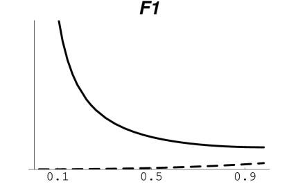
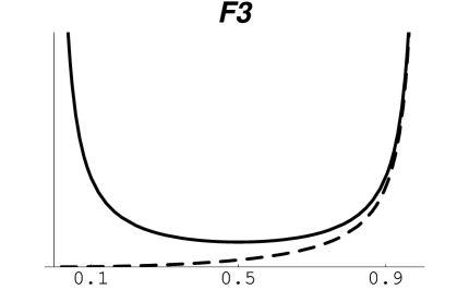
Figure 1: $F_{1}(\nu)$ (left) and $F_{3}(\nu)$ (right) without the constant first terms are shown for $0\leq\nu\leq 1$. The solid lines include the contribution of the zero Matsubara frequency, while it is subtracted in the dashed curves.

7.0.1 Electric sector without the zero Matsubara frequency contribution

The functions $F_{1}$ and $F_{2}$ have so far been evaluated by summing over all the Matsubara frequencies, including the static fluctuations around static gluon background fields. This is of interest for a number of physical cases. For the problem of dimensional reduction, however, one does not include the static quantum fluctuations. Subtracting the contributions of the zero Matsubara frequency, which are of order $1/\nu$, we obtain

$$\tilde{F}_{1}(\nu) = \frac{11}{48\pi^{2}}\left[2\textnormal{log}\,\frac{\Lambda}{4\pi T}-\psi\left(-\frac{\nu}{2}\right)-\psi\left(\frac{\nu}{2}\right)\right]\;,$$ (79)

$$\tilde{F}_{2}(\nu) = \frac{11}{48\pi^{2}}\left[\psi\left(-\frac{\nu}{2}\right)+\psi\left(\frac{\nu}{2}\right)-\psi\left(\nu\right)-\psi\left(-\nu\right)\right]\;,$$ (80)

$$\tilde{F}_{3}(\nu) = \frac{11}{48\pi^{2}}\left[2\textnormal{log}\,\frac{\Lambda}{4\pi T}-\psi\left(\nu\right)-\psi\left(-\nu\right)\right]\,.$$ (81)

Here we used the relation for the $\psi$ function: $\psi(1+\nu)=\psi(\nu)+\frac{1}{\nu}$. Keeping in mind that

$$-\psi(x)-\psi(-x)=2\left[\gamma_{E}+\zeta(3)x^{2}+\zeta(5)x^{4}+\ldots\right]$$ (82)

where $\zeta(n)$ is the Riemann zeta function, we see that the contribution of the nonzero Matsubara frequencies to the effective action is regular at $A_{4}=0$, and that the bare coupling constant should be replaced by the running one taken at the scale $4\pi e^{-\gamma_{E}}\,T\approx\!7.05551\,T$, if the Pauli-Villars $\Lambda$ is used. If another regularization scheme is used, the scale should be changed accordingly, see the Introduction.

The plots of $\tilde{F}_{1,3}$ (without the first terms) are also shown in Fig.1.

7.0.2 The ‘equation of motion’ term

We finally compute the second term in the invariant $I_{2}$, which we have so far left out. Its contribution is

$$S_{{\rm EoM}}=\frac{1}{T}\int\,d^{3}x\,\sum_{k=-\infty}^{\infty}\int\frac{d^{3}p}{(2\pi)^{3}}\,\int_{0}^{\infty}\frac{ds}{s}\,e^{-sp^{2}}\,T\,\left[-s^{2}\left(\frac{1}{2}-\frac{2}{9}sp^{2}\right)\,{\rm Tr}\,e^{s\mathcal{A}^{2}}\left(i\left\{\mathcal{A},\left[D_{i},E_{i}\right]\right\}\right)\right]\;,$$ (83)

where the curly brackets denote the anticommutator. After all integrations and the summation over $\omega_{k}$ it gives

$$S_{{\rm EoM}}=\int\,d^{3}x\,\frac{1}{12\pi}\left[\frac{(D_{i}E_{i})^{a}\,A_{4}^{a}}{\pi T}-\frac{(D_{i}E_{i})^{b}\,A_{4}^{b}}{\sqrt{A_{4}^{c}\,A_{4}^{c}}}\right]\;.$$ (84)

Here the first term comes exclusively from the nonzero Matsubara frequencies, while the second term is the contribution of the zero Matsubara frequency alone. Equation (84) is zero if the classical equation of motion is satisfied [see Appendix A]. If the background field does not satisfy the equation of motion one can integrate eq. (84) by parts which yields:

$$S_{{\rm EoM}}=\frac{1}{12\pi^{2}}\!\int\!d^{3}x\left\{E_{i}^{a}E_{i}^{a}\left(\frac{\pi}{|A_{4}|}-\frac{1}{T}\right)+\frac{\pi}{|A_{4}|^{3}}\left(E_{i}^{a}A_{4}^{a}\right)\left(E_{i}^{b}A_{4}^{b}\right)-\partial_{i}\left(E_{i}^{a}A_{4}^{a}\left(\frac{\pi}{|A_{4}|}-\frac{1}{T}\right)\right)\right\}.$$ (85)

Apart from the last term which is a full derivative the first two can be added to the functions $f_{1,2}$ found previously.

8 Magnetic sector

We are now going to calculate the fourth and fifth terms in eq. (31), i.e. terms quadratic in the magnetic field. In analogy to the derivation of the action for the electric sector, we make an expansion in the spatial covariant derivative $D_{i}$ of the functional determinants and collect powers of the magnetic field. Note that while the electric field only needed one power of a covariant derivative the magnetic field needs two. For magnetic field squared we hence need an expansion to fourth order in the covariant derivatives. In principle, in the fourth order in the covariant derivatives there is a mixed term of the type $\epsilon_{ijk}\epsilon^{abc}E_{i}^{a}E_{j}^{b}B_{k}^{c}\,f(A_{4})$, terms quartic in $E_{i}$ and terms containing covariant derivatives of $E_{i}$ but we do not consider them here. For that reason, we neglect all commutators $[D_{i},A_{4}]$, as they introduce additional powers of $E_{i}$. This simply means that we can drag all powers of the covariant derivative $D_{i}$ as well as of the field strengths $F_{ij}$ through the exponentials of $A_{4}$, as if they commute .

For the ghost determinant (57) we obtain [see Appendix C.1] only one gauge invariant structure, which after integration over $p$ becomes

$$\left[\textnormal{log}\,\textnormal{det}(-D^{2})_{\rm{r,n}}\right]_{{\rm M}}^{(2)}=\frac{1}{48\,\pi^{3/2}}\,\int\,d^{3}x\,\sum_{k=-\infty}^{\infty}\int_{0}^{\infty}\frac{ds}{\sqrt{s}}\,{\rm Tr}\left(1-e^{-sM^{2}}\right)\left(e^{s\mathcal{A}^{2}}\,B_{k}B_{k}\right)\;.$$ (86)

For the gluon determinant (59) we get the same result times a factor of $-2$ plus one additional term:

$$T_{4}\equiv{\rm Tr}\int_{0}^{1}\,d\alpha\,\int_{0}^{1-\alpha}\,d\beta\,e^{\alpha s\mathcal{A}^{2}}(2s\epsilon^{acb}F_{ij}^{c})\,e^{\beta s\mathcal{A}^{2}}(2s\epsilon^{dfe}F_{ij}^{f})\,e^{(1-\alpha-\beta)s\mathcal{A}^{2}}\;,$$ (87)

which with $F_{ij}^{a}F_{ij}^{b}=2B_{k}^{a}B_{k}^{b}$ and after integration over $\alpha$ and $\beta$ yields the same gauge invariant structure:

$$T_{4}=4\,s^{2}{\rm Tr}\left(e^{s\mathcal{A}^{2}}B_{k}B_{k}\right)\;.$$ (88)

We find [see Appendix C.1] that this term yields the same contribution to the action as the ghost determinant, but multiplied by a factor of $12$. The total contribution of the gluon determinant to the 1-loop action in the magnetic sector is hence $10$ times that of the ghost determinant.

The total 1-loop action in the magnetic sector is

$$\left[S_{\rm{1-loop}}^{(2)}\right]_{{\rm M}}=\left[\textnormal{log}\,\left(\textnormal{det}{W}\right)^{-1/2}_{{\rm r,n}}+\textnormal{log}\,\textnormal{det}\left({-D^{2}}\right)_{{\rm r,n}}\right]^{(2)}_{{\rm M}}$$

$$=\frac{11}{48\,\pi^{3/2}}\,\int\,d^{3}x\,\sum_{k=-\infty}^{\infty}\int_{0}^{\infty}\frac{ds}{\sqrt{s}}\,{\rm Tr}\left(1-e^{-sM^{2}}\right)\left(e^{s\mathcal{A}^{2}}\,B_{k}B_{k}\right)\,,$$

where the integration over $s$ and the summation over Matsubara frequencies still have to be performed. However, we do not need to do it anew since exactly the same gauge invariant appeared in the invariant $I_{2}$ in the electric sector, with the obvious replacement $E_{i}\to B_{i}$, see eq. (62). With our gauge choice we obtain two structures, $(B_{i}^{1}B_{i}^{1}+B_{i}^{2}B_{i}^{2})\,h_{1}(\nu)$ and $B_{i}^{3}B_{i}^{3}\,h_{3}(\nu)$, which can be written in invariant terms as

$$B_{i}^{2}h_{1}(\nu)\qquad{\rm and}\qquad\frac{(B_{i}\cdot A_{4})^{2}}{|A_{4}|^{2}}\left(h_{3}(\nu)-h_{1}(\nu)\right)\;,$$ (90)

respectively.

Combining the ghost and the gluon result and denoting $(h_{3}-h_{1})$ by $h_{2}$ we find the two functions defined in eq.(31):

$$h_{1}(\nu) = \frac{f_{3}(\nu)}{2}+\frac{11}{48\,\pi^{2}}\textnormal{log}\,\mu=\frac{11}{96\pi^{2}}\left[4\left(\textnormal{log}\,\frac{M}{4\pi T}+\frac{\gamma_{{\rm E}}}{2}\right)-\psi\left(\nu\right)-\psi\left(1-\nu\right)\right]\,,$$ (91)

$$h_{2}(\nu) = \frac{f_{3}(\nu)}{2}-\frac{11}{48\,\pi^{2}}\textnormal{log}\,\mu=-\frac{11}{96\pi^{2}}\left[2\gamma_{{\rm E}}+\psi\left(\nu\right)+\psi\left(1-\nu\right)\right]\,,$$ (92)

$$h_{3}(\nu) = f_{3}(\nu)=\frac{11}{48\pi^{2}}\left[2\textnormal{log}\,\frac{M}{4\pi T}-\psi\left(\nu\right)-\psi\left(1-\nu\right)\right]\,,\qquad\nu=\frac{\sqrt{A_{4}^{a}A_{4}^{a}}}{(2\pi T)}\,.$$ (93)

As before $\mu$ is given by eq. (71).

The UV divergent logarithm in eq. (91) cancels the divergence from the tree-level action which has the running coupling defined at the cutoff momentum $M$,

$$\frac{B_{i}^{a}B_{i}^{a}}{2g^{2}(M)}=B_{i}^{a}\,B_{i}^{a}\,\frac{11}{24\pi^{2}}\,\textnormal{log}\frac{M}{\Lambda}\;,$$ (94)

such that the sum of tree and 1-loop actions are UV finite. The finite full action can be brought into the form of eq.(3) where the functions $H_{1,2,3}$ are obtained from $h_{1,2,3}$ by replacing the cutoff $M$ by $\Lambda$:

$$H_{1}(\nu) = \frac{F_{3}(\nu)}{2}+\frac{11}{48\,\pi^{2}}\textnormal{log}\,\mu=\frac{11}{96\pi^{2}}\left[4\left(\textnormal{log}\,\frac{\Lambda}{4\pi T}+\frac{\gamma_{{\rm E}}}{2}\right)-\psi\left(\nu\right)-\psi\left(1-\nu\right)\right]\;,$$ (95)

$$H_{2}(\nu) = \frac{11}{96\pi^{2}}\left[2\gamma_{{\rm E}}-\psi\left(\nu\right)-\psi\left(1-\nu\right)\right]\,,$$ (96)

$$H_{3}(\nu) = F_{3}(\nu)=\frac{11}{48\pi^{2}}\left[2\textnormal{log}\,\frac{\Lambda}{4\pi T}-\psi\left(\nu\right)-\psi\left(1-\nu\right)\right]\,,\qquad\nu=\frac{\sqrt{A_{4}^{a}A_{4}^{a}}}{(2\pi T)}\,.$$ (97)

When we sum over the Matsubara frequencies we find as in the case of the electric sector, that the zero Matsubara frequency contributes both with a finite term which is proportional to $1/\phi$ and a ‘naked’ IR divergent part. The finite terms are included in the results (91) and (92). The separate contribution of the IR divergent part is

$$\lim_{\omega_{k}\to 0}\frac{1}{\pi}\frac{11}{48}\int\,d^{3}x\,\left(B_{k}^{a}B_{k}^{a}-\frac{(B_{i}\cdot A_{4})^{2}}{|A_{4}|^{2}}\right)\,\frac{1}{\omega_{k}}\;.$$ (98)

In contrast to the electric sector, this divergence does not get canceled. This is also clearly seen in terms of Feynman diagrams and corresponds to a singularity in the magnetic self-energy of the gluons due to the zero Matsubara frequency in the loop, when the external gluons have zero momentum. This singularity is regularized when higher terms in $B_{i}$ and/or nonzero momenta of the background magnetic field are taken into account.

8.0.1 Magnetic sector without the zero Matsubara frequency contribution

For a discussion of dimensional reduction at high temperatures we again remove the contribution of the zero Matsubara frequency and obtain:

$$\tilde{H}_{1}(\nu) = \frac{11}{96\pi^{2}}\left[4\left(\textnormal{log}\,\frac{\Lambda}{4\pi T}+\frac{\gamma_{{\rm E}}}{2}\right)-\psi\left(\nu\right)-\psi\left(-\nu\right)\right]\;,$$ (99)

$$\tilde{H}_{2}(\nu) = -\frac{11}{96\pi^{2}}\left[2\gamma_{{\rm E}}+\psi\left(\nu\right)+\psi\left(-\nu\right)\right]\;,$$ (100)

$$\tilde{H}_{3}(\nu) = \frac{11}{48\pi^{2}}\left[2\textnormal{log}\,\frac{\Lambda}{4\pi T}-\psi\left(\nu\right)-\psi\left(-\nu\right)\right]\;.$$ (101)

The IR singularity (98) is of course not present.

9 Comparison of our results to previous work

There have been two other publications with the aim to get an effective theory for QCD at high temperatures. In the first one [25] gluon by gluon scattering at low momenta in the nonzero temperature Yang-Mills theory is calculated in terms of Feynman diagrams. In the second one [13] an effective theory for the static modes of $SU(N)$ Yang–Mills theory in terms of a covariant derivative expansion is derived. The author makes a series expansion of the functional determinants, and goes up to six orders in the covariant derivative. This corresponds to a 1-loop calculation with up to six external static gluons and their effective vertices. The zero Matsubara frequency contribution is not included.

To compare our results to those of Refs.[25] and [13] we need to expand our functions $f_{1,2}$, $h_{1,2}$ in powers of $A_{4}$. We would like to stress that within our calculation we can go to arbitrary power of $A_{4}$, while Refs. [25] and [13] only go to the quadratic order. For a comparison we look at the quadratic terms in $A_{4}$ and obtain the following contribution:

$$\int\,d^{3}x\,\frac{\zeta(3)}{\pi^{4}T^{3}}\frac{11}{384}\left(E^{2}A_{4}^{2}+3(EA_{4})^{2}\right)\;.$$ (102)

This agrees precisely with Ref. [13] after collecting terms of the orders above. Ref.[25] differs both in sign and magnitude. For the magnetic part we can only compare to Ref. [13], as only there the terms under consideration have been computed. To quadratic order in $A_{4}$ we obtain

$$\int\,d^{3}x\,\frac{\zeta(3)}{\pi^{4}T^{3}}\frac{11}{192}\left(B^{2}A_{4}^{2}+(BA_{4})^{2}\right)\;,$$ (103)

which again coincides exactly with the result derived in Ref. [13]. In addition, in Ref. [14] the 1-loop action for the Polyakov line has been computed up to two derivatives in the specific case of zero $A_{i}$. Although it may look as being a gauge-noninvariant condition, in fact one of the gauge-invariant structures can be extracted from that calculation. Indeed, the gauge-invariant combination $(E_{i}A_{4})^{2}/A_{4}^{2}$ projects out the $A_{i}$ field. Therefore, what we call the $f_{3}$ function has been actually computed in that paper, and our result coincides with theirs.

10 Time dependence and periodicity in $A_{4}$

So far we have considered only time-independent background fields $A_{4}$ and $A_{i}$. As stressed in the Introduction, taking $A_{4}$ static is no restriction on the background but merely a convenient gauge choice. However, taking $A_{i}$ static is a restriction, and we would like to relax it, that is to include terms in the effective action containing time derivatives $\dot{A}_{i}$. To the second order in $\dot{A}_{i}$, this can be done in a very simple way. Namely, we notice that in deriving the quantum action we have made use of the commutators (54,55) which remain exactly the same if we replace $A_{4}$ in $\mathcal{A}$ by the more general operator $D_{4}$. The only difference is that the resulting electric field should be now understood as the full $E_{i}^{a}=D_{i}^{ab}A_{4}^{b}-\dot{A}_{i}^{a}$. With this replacement, one gets the same effective action (3) as in the case of a purely static $A_{i}$. As in the static case, it is limited to the second power of $E_{i}$ and hence of $\dot{A}_{i}$. Therefore, its applicability is restricted by the condition that both spatial and time derivatives of the fields are much less than the temperature.

After fixing the gauge such that $A_{4}$ is static one can perform further a time-independent gauge rotation to make $A_{4}(x)$ diagonal i.e. belonging to the Cartan subalgebra at all spatial points. We shall use this gauge condition in this section to simplify the discussion. For the $SU(2)$ gauge group it means that we take $A_{4}=\phi\,\frac{\tau^{3}}{2}$.

Having fixed the gauge such that $A_{4}$ is static and diagonal there is only an Abelian residual gauge symmetry left. It consists of arbitrary time-independent gauge rotations about the Cartan generators, and of a timedependent gauge rotation (also about the Cartan axes) of a special discrete type compatible with periodicity of $A_{i}(x,t)$. For the $SU(2)$ gauge group this residual gauge symmetry is with respect to the Abelian gauge transformation

$$A_{\mu}\to S^{\dagger}A_{\mu}S+iS^{\dagger}\partial_{\mu}S,\qquad S(x,t)=\textnormal{exp}\left\{-i\frac{\tau^{3}}{2}\left[\alpha(x)+2\pi tTn\right]\right\},$$ (104)

where $n$ is an integer, which follows from the requirement that $A_{i}(x,t)$ remains periodic in time. One cannot take rotations about axes other than the $3^{\rm d}$ one because it will make $A_{4}$ nondiagonal, and one cannot take the time dependence other than linear because that would make $A_{4}$ timedependent. In components, the transformation (104) reads:

$$A_{4}^{\prime\,3}(x) = A_{4}^{3}(x)+2\pi T\,n,\qquad{\rm meaning}\quad\nu^{\prime}=\nu+n,$$ (105)

$$A_{i}^{\prime\,1}(x,t) = {\rm cos}\beta A_{i}^{1}+{\rm sin}\beta A_{i}^{2},\qquad\beta(x,t)=\alpha(x)+2\pi Tnt,$$ (106)

$$A_{i}^{\prime\,2}(x,t) = -{\rm sin}\beta A_{i}^{1}+{\rm cos}\beta A_{i}^{2},$$ (107)

$$A_{i}^{\prime\,3}(x,t) = A_{i}^{3}+\partial_{i}\alpha(x).$$ (108)

The effective action must be invariant under this transformation, but is it?

It is easy to check that the combinations of the field strengths $B_{i}^{3}B_{i}^{3}$, $B_{i}^{\perp}B_{i}^{\perp}$, $E_{i}^{3}E_{i}^{3}$ and $E_{i}^{\perp}E_{i}^{\perp}$ (where $F^{\perp}F^{\perp}$ is the short-hand notation for $F^{1}F^{1}+F^{2}F^{2}$) are invariant under the gauge transformation (105-108). As follows from eq. (3) these structures are multiplied by the functions $H_{3}(\nu),H_{1}(\nu),F_{3}(\nu)$ and $F_{1}(\nu)$, respectively. Therefore to support the invariance of the effective action under the gauge transformation (104), all the four functions need to be periodic in $\nu=A_{4}^{3}/2\pi T$ with unit period.

So far we have computed those functions in the domain $0<\nu<1$, so to check the periodicity one has to know them outside this domain. Actually only the last step, namely the summation over Matsubara frequencies, has to be revisited. The result is as follows: The static potential $V(\nu)$ and the functions $H_{1}(\nu),H_{3}(\nu)$ and $F_{3}(\nu)$ are, indeed, periodic (and even) in $\nu$, whereas the last function $F_{1}(\nu)$ is even but not periodic.

Indeed, for $0<|\nu|<1$ we find:

$$F_{1}(\nu)=-\frac{11}{48\pi^{2}}\left[L+\psi\left(\frac{\nu}{2}\right)+\psi\left(-\frac{\nu}{2}\right)-\frac{20}{11|\nu|}\right]\;.$$ (109)

For $1<|\nu|<2$ we find:

$$F_{1}(\nu)=-\frac{11}{48\pi^{2}}\left[L+\psi\left(\frac{\nu}{2}\right)+\psi\left(-\frac{\nu}{2}\right)-2-\frac{38}{11\nu}-\frac{8}{11}\left(\frac{1}{\nu^{2}}-\frac{1}{|\nu^{3}|}\right)\right]\;.$$ (110)

For $2<|\nu|<3$ we find:

$$F_{1}(\nu)=-\frac{11}{48\pi^{2}}\left[L+\psi\left(\frac{\nu}{2}\right)+\psi\left(-\frac{\nu}{2}\right)-3-\frac{56}{11|\nu|}-\frac{24}{11\nu^{2}}-\frac{40}{11|\nu^{3}|}+\frac{2}{2-|\nu|}+\frac{2}{4-|\nu|}\right]\,,$$ (111)

etc. By $L$ we have denoted the constant part: $L=-2\textnormal{log}(\Lambda/4\pi T)$.This function is plotted in Fig. 2 and is clearly not periodic.

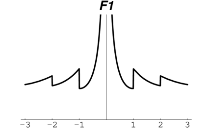
Figure 2: The function $F_{1}(\nu)$ with the constant part $L$ subtracted, in different intervals.

The reason of this periodicity paradox is clear. By making the timedependent gauge transformation (105-108) we induce large time derivatives of the $A_{i}^{1,2}$ fields, being of the order of $2\pi T$. The ‘dynamical’ electric field $\dot{A}_{i}^{1,2}$ does not enter into the invariants $B_{i}^{3}B_{i}^{3}$, $B_{i}^{\perp}B_{i}^{\perp}$ and $E_{i}^{3}E_{i}^{3}$. Therefore, the corresponding functions $H_{1}(\nu),H_{3}(\nu)$ and $F_{3}(\nu)$ should be periodic to support gauge invariance, which indeed they are. One cannot and should not observe gauge invariance in the structure $E_{i}^{\perp}E_{i}^{\perp}\,F_{1}(\nu)$ as it is only a quadratic functional in $\dot{A}_{i}^{1,2}$, which is insufficient. There is no periodicity requirement on $F_{1}(\nu)$. All powers of $\dot{A}_{i}^{1,2}/T$ (and of $A_{4}/T$) need to be collected in the effective action to check the invariance under fast timedependent gauge transformations (104). This, however, lies beyond the scope of the present study.

11 Conclusions

Given that the Polyakov line in the $A_{4}$ static gauge is

$$P(x)=\textnormal{exp}\left(i\frac{A_{4}(x)}{T}\right),$$ (112)

its gauge-invariant eigenvalues are $e^{\pm i\pi\nu}$ where $\nu=\sqrt{A_{4}^{a}A_{4}^{a}}/2\pi T$. We have in fact computed the 1-loop effective action for the eigenvalues of the Polyakov line, interacting with the spatial components of the Yang–Mills field $A_{i}$. For the $SU(2)$ gauge group the effective action is given by eq. (3) with the four functions $F_{1,2}(\nu)$ and $H_{1,2}(\nu)$ defined in eqs.(76, 77) and eqs.(95, 96), respectively. All functions are singular and behave as $1/A_{4}$ at small $A_{4}$, which is due to the contribution of the zero Matsubara frequency. It should be stressed that the functions $H_{1,2}(\nu)$ being coefficients in front of the invariants quadratic in the magnetic field, contain ‘naked’ IR divergences which are regularized by higher orders of the magnetic field and/or field momentum. If the static fluctuation mode is excluded from the effective action, all functions become finite and nonsingular; they are then given by eqs.(79, 80) and eqs.(99, 100), respectively. If the background field does not satisfy the Yang–Mills equations of motion, there is an additional term (84).

As it should be expected, the functions $H_{1,2}(\nu),\,F_{3}(\nu)=F_{1}(\nu)+F_{2}(\nu)$ and the static potential $V(\nu)$ are periodic functions of $\nu$ but $F_{1}(\nu)$ is not. The periodicity is related to the gauge invariance of the effective action with respect to fast timedependent gauge transformations inducing large electric field $\dot{A}_{i}$. For the particular structure related to $F_{1}(\nu)$, this gauge invariance can only be revealed when all powers of the electric field in the effective action are collected.

For higher gauge groups there will be more invariant structures already in the quadratic order in the electric and magnetic fields, and the coefficient functions will depend on all the eigenvalues of the Polyakov line, whose number is $N-1$ for the $SU(N)$ gauge group. It is worthwhile to generalize this work to higher groups, as well as to find the 1-loop affective action arising from integrating out fermions.

One can think of two kinds of applications of our results. One is for studying correlation functions, say, of the Polyakov lines at high temperatures but going beyond the approximations used previously. One might be also interested in evaluating the 1-loop weights of extended semiclassical objects, such as calorons with nontrivial holonomy and dyons. The technique developed in this paper is applicable for such studies.

Acknowledgments:
We are grateful to Rob Pisarski for valuable discussions and to Eric Braaten for reading the manuscript and helpful comments. D.D. would like to thank Victor Petrov and M.O. would like to thank Jonathan Lenaghan for useful conversations at the early stage of this work.

M.O. thanks Brookhaven National Laboratory for its hospitality and was partly supported by the U.S. Department of Energy under Contract No. DE-AC02-98CH10886.

Appendix A Notations

We normalize the generators of an SU(N) group as

$${\rm Tr}\,t^{a}\,t^{b}=\frac{1}{2}\,\delta^{ab}\;.$$ (113)

For SU(2) $t^{a}$ are half the Pauli matrices, and for SU(3) half the Gell-Mann matrices. Their commutator defines the generators of the adjoint representation:

$$(T_{a})^{bc}=-i\,f^{abc}=i\,f^{acb}\;.$$ (114)

The field strength in the fundamental representation is defined as

$$[\nabla_{\mu},\nabla_{\nu}]=-i\,F_{\mu\nu}=-i\,F_{\mu\nu}^{a}\,t^{a}\;,$$ (115)

where

$$\nabla_{\mu}=\partial_{\mu}-i\,A_{\mu}^{a}\,t^{a}\;,$$ (116)

is the covariant derivative in the fundamental representation.

The field strength in adjoint representation becomes

$$[D_{\mu},D_{\nu}]^{cd}=-f^{cda}\,F_{\mu\nu}^{a}=f^{cad}\,F_{\mu\nu}^{a}\;,$$ (117)

where $D_{\mu}$ is the covariant derivative in the adjoint representation:

$$D_{\mu}^{ab}=\partial_{\mu}\delta^{ab}+f^{acb}\,A_{\mu}^{c}\;.$$ (118)

For any matrix in the adjoint representation we shall imply $B^{ab}=-i\,f^{abc}\,B^{c}$. In particular, the gauge field which in the fundamental representation is $A_{\mu}=A_{\mu}^{a}\,t^{a}$ becomes in the adjoint representation

$$A_{\mu}^{cd}=-i\,f^{cde}\,A_{\mu}^{e}=i\,f^{ced}\,A_{\mu}^{e}\;.$$ (119)

The electric field is in general defined as $E_{i}\equiv F_{i4}$. Hence

$$[D_{i},D_{4}]=-i\,F_{i4}=-i\,E_{i}\;.$$ (120)

Explicitly in the adjoint representation one has

$$E_{i}^{ab}=-i\,f^{abd}D_{i}^{dh}A_{4}^{h}=-i\,f^{abd}E_{i}^{d}\qquad{\rm and}\qquad E_{i}^{d}=D_{i}^{dh}A_{4}^{h}\;.$$ (121)

We notice that the combination

$$[D_{i},E_{i}]^{ab}=-if^{abe}\,D_{i}^{ec}\,E_{i}^{c}\;$$ (122)

is zero if the background field satisfies the Yang–Mills equation of motion, $D_{\mu}^{ac}F_{\mu\nu}^{c}=0$. For eq. (122) we use the Jacobi identity

$$f^{abe}f^{efc}=f^{afe}f^{ebc}-f^{ace}f^{ebf}\;.$$ (123)

Appendix B Functional determinants in the electric sector

B.1 Managing functional traces

We are interested here in extracting terms quadratic in the electric field but having any power of $A_{4}$. We expand the ghost functional determinant (57) to quadratic order in $D_{i}$ with the help of eq. (52) and obtain two contributions at this order:

$$T_{1}={\rm Tr}\int_{0}^{1}\,d\alpha\,e^{\alpha s\mathcal{A}^{2}}sD_{i}^{2}\,e^{(1-\alpha)s\mathcal{A}^{2}}\;,$$ (124)

and

$$T_{2}=-\frac{4}{3}s^{2}p^{2}{\rm Tr}\int_{0}^{1}d\alpha\int_{0}^{1-\alpha}d\beta\,e^{\alpha s\mathcal{A}^{2}}D_{i}\,e^{\beta s\mathcal{A}^{2}}D_{i}\,e^{(1-\alpha-\beta)s\mathcal{A}^{2}}\;,$$ (125)

where for $T_{2}$ we used the fact that $p_{i}p_{j}$ averaged over the directions of the three-vector $p_{i}$ gives $\frac{1}{3}\delta_{ij}p^{2}$. With the commutators (53) and (54) it can be shown that $T_{1}$ is a sum of four terms, two of which are gauge invariant and two are not gauge invariant (denoted by a bar):

$$T_{1}=T_{11}+T_{12}+\bar{T}_{11}+\bar{T}_{12}\;,$$ (126)

where

$$T_{11} = -s^{2}\int_{0}^{1}d\alpha\,(1-\alpha){\rm Tr}\,e^{s\mathcal{A}^{2}}\left(2E_{i}^{2}+i\left\{\mathcal{A},\left[D_{i},E_{i}\right]\right\}\right)\;,$$ (127)

$$T_{12} = -2s^{3}\int_{0}^{1}d\alpha\int_{0}^{1}d\gamma\int_{0}^{1}d\delta\,(1-\alpha)^{2}(1-\gamma){\rm Tr}\,e^{s\mathcal{A}^{2}[1-\delta(1-\gamma)(1-\alpha)]}\left\{\mathcal{A},E_{i}\right\}e^{s\mathcal{A}^{2}\delta(1-\gamma)(1-\alpha)}\left\{\mathcal{A},E_{i}\right\}\;$$

$$\bar{T}_{11} = s\,{\rm Tr}\left(e^{s\mathcal{A}^{2}}D^{2}\right)\;,$$

$$\bar{T}_{12} = -2is^{2}\int_{0}^{1}d\alpha\int_{0}^{1}d\gamma\,(1-\alpha){\rm Tr}\,e^{s\mathcal{A}^{2}[\alpha+\gamma(1-\alpha)]}\left\{\mathcal{A},E_{i}\right\}e^{s\mathcal{A}^{2}(1-\gamma)(1-\alpha)}D_{i}\;.$$

As the action is gauge invariant, we expect the not gauge invariant terms to cancel with those of the term $T_{2}$. We will show, that this is indeed the case.

Let us now turn to $T_{2}$. Dragging $D_{i}$’s to the right we obtain:

$$T_{2}= - \frac{4}{3}s^{2}p^{2}\int_{0}^{1}d\alpha\int_{0}^{1-\alpha}d\beta\,e^{(1-\alpha)s\mathcal{A}^{2}}D^{2}\,e^{\alpha s\mathcal{A}^{2}}$$ (128)

$$+ \frac{4i}{3}s^{3}p^{2}\int_{0}^{1}d\alpha\int_{0}^{1-\alpha}d\beta\,\beta\int_{0}^{1}d\gamma\,{\rm Tr}\,e^{(1-\alpha-\beta+\gamma\beta)s\mathcal{A}^{2}}\left\{\mathcal{A},E_{i}\right\}e^{(1-\gamma)\beta s\mathcal{A}^{2}}$$

$$\times \left\{e^{\alpha s\mathcal{A}^{2}}D_{i}-is\alpha\int_{0}^{1}d\gamma\,e^{\delta\alpha s\mathcal{A}^{2}}\left\{\mathcal{A},E_{i}\right\}e^{(1-\delta)\alpha s\mathcal{A}^{2}}\right\}\;.$$

We find that $T_{2}$ is a sum of six terms, amongst which three are gauge invariant and three (again denoted by a bar) are not. We start with the not gauge invariant ones and show that they cancel with $\bar{T}_{11}$ and $\bar{T}_{12}$

$$\bar{T}_{21} = -\frac{2}{3}s^{2}p^{2}{\rm Tr}\,\left(e^{s\mathcal{A}^{2}}D^{2}\right),$$ (130)

$$\bar{T}_{22a} = \frac{8i}{3}s^{3}p^{2}\int_{0}^{1}d\alpha\,\alpha(1-\alpha)\int_{0}^{1}d\gamma\,{\rm Tr}\,e^{s\mathcal{A}^{2}[\alpha+\gamma(1-\alpha)]}\left\{\mathcal{A},E_{i}\right\}e^{s\mathcal{A}^{2}(1-\gamma)(1-\alpha)}\,D_{i},$$ (131)

$$\bar{T}_{22b} = \frac{4i}{3}s^{3}p^{2}\int_{0}^{1}d\alpha\int_{0}^{1-\alpha}d\beta\,\beta\int_{0}^{1}d\gamma\,{\rm Tr}\,e^{s\mathcal{A}^{2}(1-\alpha-\beta+\gamma\beta)}\left\{\mathcal{A},E_{i}\right\}\,e^{s\mathcal{A}^{2}[\alpha+\beta(1-\gamma)]}\,D_{i}\,.$$ (132)

The terms $\bar{T}_{11}$ from eq. (127) and $\bar{T}_{21}$ are of the same structure. Their sum is

$$\bar{T}_{11}+\bar{T}_{21}=s\left[1-\frac{2sp^{2}}{3}\right]\,\left(e^{s\mathcal{A}^{2}}D^{2}\right)\;.$$ (133)

This term vanishes upon $p$ integration since:

$$\int_{0}^{\infty}d^{3}p\,sp^{2}\,e^{-sp^{2}}=\frac{3}{2}\int_{0}^{\infty}d^{3}p\,e^{-sp^{2}}\;.$$ (134)

For the evaluation of the other non gauge-invariant terms we use some relations for integrations over parameters, valid for any function $f$:

$$\int_{0}^{1}d\alpha\int_{0}^{1}d\gamma\,\alpha(1-\alpha)\,f(\underbrace{\alpha\gamma}_{\epsilon}) = \int_{0}^{1}d\epsilon\,\frac{(1-\epsilon)^{2}}{2}f(\epsilon)\;,$$ (135)

$$\int_{0}^{1}d\alpha\int_{0}^{1}d\gamma\,\alpha\,f(\underbrace{\alpha\gamma}_{\eta}) = \int_{0}^{1}d\eta\,(1-\eta)\,f(\eta)\;,$$ (136)

$$\int_{0}^{1}d\alpha\int_{0}^{1-\alpha}d\beta\beta\int_{0}^{1}d\gamma\,f(\underbrace{\alpha+\beta\gamma}_{\delta}) = \int_{0}^{1}d\delta\,\delta(1-\delta)\,f(\delta)\;.$$ (137)

We find that

$$\!\!\!\bar{T}_{12}\!+\!\bar{T}_{22a}\!+\!\bar{T}_{22b}\!\!=\!\!\int_{0}^{1}\!\!d\alpha\!\!\left[-2is^{2}(1\!-\!\alpha)\!\!+\!\!\frac{4i}{3}s^{3}p^{2}(1\!-\!\alpha)^{2}\!\!+\!\!\frac{4i}{3}s^{3}p^{2}\alpha(1\!-\!\alpha)\right]\!{\rm Tr}\,e^{s\mathcal{A}^{2}(1\!-\!\alpha)}\!\!\left\{\mathcal{A},E_{i}\right\}\!e^{s\mathcal{A}^{2}\alpha}D_{i}\;.$$ (138)

After integration over $\alpha$ the term in the brackets

$$\left[\ldots\right]=-is^{2}\left(1-\frac{2}{3}sp^{2}\right)$$ (139)

becomes zero after integration over $p$. We hence have shown that all not gauge invariant terms cancel out, as was indeed expected.

There are three gauge invariant terms left. They can be simplified by using some more integration relations:

$$\int_{0}^{1}d\alpha\,\alpha^{2}(1-\alpha)\int_{0}^{1}d\gamma\,\gamma\int_{0}^{1}d\delta\,f(\underbrace{\alpha\gamma\delta}_{\xi}) = \frac{1}{6}\int_{0}^{1}d\xi\,(1-\xi)^{3}\,f(\xi)\;,$$ (140)

$$\int_{0}^{1}d\alpha\,\alpha\int_{0}^{1-\alpha}d\beta\,\beta\int_{0}^{1}d\gamma\int_{0}^{1}d\delta\,f(\underbrace{\alpha\delta+\beta\gamma}_{\zeta}) = \int_{0}^{1}\,\frac{\zeta(1-\zeta)^{2}}{2}\,f(\zeta)\;,$$ (141)

$$\int_{0}^{1}d\alpha\,\alpha^{2}\int_{0}^{1}d\gamma\,\gamma\int_{0}^{1}d\delta\,f(\underbrace{\alpha\gamma\delta}_{\kappa}) = \frac{1}{2}\int_{0}^{1}d\kappa\,(1-\kappa)^{2}\,f(\kappa)\;.$$ (142)

Using them we find two gauge invariant structures

$$I_{1} \equiv T_{12}+T_{22a}+T_{22b}$$

$$= s^{3}\int_{0}^{1}d\alpha\,\left\{-\frac{1}{2}+\alpha(1-\alpha)+\frac{2}{9}sp^{2}\left[1-\frac{3}{2}\alpha(1-\alpha)\right]\right\}\,{\rm Tr}\,e^{(1-\alpha)s\mathcal{A}^{2}}\left\{\mathcal{A},E_{i}\right\}\,e^{\alpha s\mathcal{A}^{2}}\,\left\{\mathcal{A},E_{i}\right\}\;,$$

$$I_{2} \equiv T_{11}+T_{21}=-s^{2}\left(\frac{1}{2}-\frac{2}{9}sp^{2}\right)\,{\rm Tr}\,e^{s\mathcal{A}^{2}}\left(2E_{i}^{2}+i\left\{\mathcal{A},\left[D_{i},E_{i}\right]\right\}\right)\;.$$ (144)

In the evaluation of the gluon determinant (59) there is one more gauge invariant structure:

$$I_{3}\equiv T_{3} = -2\int_{0}^{1}\,d\alpha\int_{0}^{1-\alpha}\,d\beta\,{\rm Tr}\,e^{\alpha s\mathcal{A}^{2}}\,(2sE_{i})\,e^{\beta s\mathcal{A}^{2}}(2sE_{i})\,e^{(1-\alpha-\beta)s\mathcal{A}^{2}}$$ (145)

$$= -4s^{2}\int_{0}^{1}\,d\alpha\,{\rm Tr}\,e^{(1-\alpha)s\mathcal{A}^{2}}E_{i}\,e^{\alpha s\mathcal{A}^{2}}E_{i}\;.$$ (146)

B.2 Integrating over $\alpha$, $s$, $p$ and summing over Matsubara frequencies

To obtain the action we have to integrate over $\alpha$, $s$, momentum $p$ and sum over Matsubara frequencies $\omega_{k}$ for the three invariants we derived. For convenience we take out a factor of $1/(2\pi^{2}T)$:

$$\frac{1}{2\pi^{2}T}\int\,d^{3}x\,\sum_{k=-\infty}^{\infty}\int\frac{d^{3}p}{(2\pi)^{3}}\,\int_{0}^{\infty}\frac{ds}{s}\,e^{-sp^{2}}\,2\pi^{2}T\,I_{j}\qquad{{\rm where}}\qquad\qquad{j=1,2,3}\qquad\;.$$ (147)

B.2.1 The first invariant $I_{1}$

After taking the trace in eq. (B.1) explicitly and integrating over $\alpha$ we find that $I_{1}$ has the structure:

$$2\pi^{2}T\,I_{1}=X_{1}\,(E_{i}^{1}\,E_{i}^{1}+E_{i}^{2}\,E_{i}^{2})+X_{3}\,E_{i}^{3}\,E_{i}^{3}\;.$$ (148)

This is expected since our gauge choice for $A_{4}$ is along the third color direction, so the result should by symmetric in $E^{1,2}$. Next we integrate over momentum, using that $d^{3}p=4\pi\,p^{2}\,dp$. We find

$$2\pi^{2}P_{1} \equiv \int_{0}^{\infty}dp\,p^{2}\,X_{1}=p_{10}\,e^{-s\omega_{k}^{2}}+p_{1p}\,e^{-s(\phi+\omega_{k})^{2}}+p_{1m}\,e^{-s(\phi-\omega_{k})^{2}}\;,$$ (149)

$$2\pi^{2}P_{3} \equiv \int_{0}^{\infty}dp\,p^{2}\,X_{3}=p_{3p}\,e^{-s(\phi+\omega_{k})^{2}}+p_{3m}\,e^{-s(\phi-\omega_{k})^{2}}\;,$$ (150)

where the coefficients are:

$$p_{10} = \frac{\sqrt{\pi}\,(-3+s\phi^{2})}{12\,s^{3/2}\,\phi^{2}}-\frac{\sqrt{\pi}}{4\,s^{5/2}\,\phi^{3}\,(-\phi+2\omega_{k})}+\frac{\sqrt{\pi}}{4\,s^{5/2}\,\phi^{3}\,(\phi+2\omega_{k})}\;,$$ (151)

$$p_{1p} = -\frac{\sqrt{\pi}\,(3+s\phi^{2})}{24\,s^{3/2}\,\phi^{2}}-\frac{\sqrt{\pi}\,\omega_{k}}{12\,\sqrt{s}\,\phi}-\frac{\sqrt{\pi}}{4\,s^{5/2}\,\phi^{3}\,(\phi+2\omega_{k})}\;,$$ (152)

$$p_{1m} = -\frac{\sqrt{\pi}\,(3+s\phi^{2})}{24\,s^{3/2}\,\phi^{2}}+\frac{\sqrt{\pi}\,\omega_{k}}{12\,\sqrt{s}\,\phi}+\frac{\sqrt{\pi}}{4\,s^{5/2}\,\phi^{3}\,(-\phi+2\omega_{k})}\;,$$ (153)

$$p_{3p} = \frac{\sqrt{s\,\pi}\,(\phi+\omega_{k})^{2}}{12}\;,$$ (154)

$$p_{3m} = \frac{\sqrt{s\,\pi}\,(\phi-\omega_{k})^{2}}{12}\;.$$ (155)

Next we integrate over $s$. The integrals over $s$ of the individual terms in $P_{1}$ turn out to be UV divergent. however their sum is finite. Using a regularization, i.e. replacing the integration kernel $P_{1}$ by $\lim_{\epsilon\to 0}\left(P_{1}\cdot s^{\epsilon}\right)$ we find the finite result:

$$S_{1} \equiv \lim_{\epsilon\to 0}\int_{0}^{\infty}ds\,\left(P_{1}\cdot s^{\epsilon}\right)=\frac{\pi\,|\omega_{k}|\,(\phi^{4}+2\,\phi^{2}\,\omega_{k}^{2}-16\,\omega_{k}^{2})}{12\,\phi^{2}\,\omega_{k}^{2}\,(\phi^{2}-4\,\omega_{k}^{2})}-\frac{\pi\,(\phi+2\,\omega_{k})}{24\,\phi\,|\phi+\omega_{k}|}$$

$$+ \frac{\pi\,|\phi+\omega_{k}|}{4\,\phi^{2}}-\frac{\pi\,|\phi+\omega_{k}|^{3}}{3\,\phi^{3}\,(\phi+2\,\omega_{k})}-\frac{\pi\,(\phi-2\,\omega_{k})}{24\,\phi\,|\phi-\omega_{k}|}+\frac{\pi\,|\phi-\omega_{k}|}{4\,\phi^{2}}-\frac{\pi\,|\phi-\omega_{k}|^{3}}{3\,\phi^{3}\,(\phi-2\,\omega_{k})}\;.$$

The integral over $P_{3}$ is finite and we obtain

$$S_{3}\equiv\int_{0}^{\infty}ds\,P_{3}=\frac{\pi\,(\phi-\omega_{k})^{2}}{24\,|\phi-\omega_{k}|^{3}}+\frac{\pi\,(\phi+\omega_{k})^{2}}{24\,|\phi+\omega_{k}|^{3}}\;.$$ (157)

The next and final step is to sum over the Matsubara frequencies. We replace $\omega_{k}$ once by $2\pi Tk$ and once by $-2\pi Tk$, where $k\geq 1$, and add the two results, which has the advantage, that we have to sum over the positive frequencies only. The zero Matsubara frequency will be treated separately. The field variable is rescaled according to

$$\phi=2\pi T\nu\qquad{{\rm where}}\qquad 0\leq\nu\leq 1\;.$$ (158)

This results into

$$TS_{1}^{\prime} = \frac{1}{12k}+\frac{1}{12(\nu-2k)}-\frac{1}{24(\nu-k)}+\frac{1}{24(\nu+k)}-\frac{1}{12(\nu+2k)}$$ (159)

$$TS_{3}^{\prime} = \frac{1}{24(\nu+k)}-\frac{1}{24(\nu-k)}\;,$$ (160)

where the prime indicates, that this is valid for nonzero Matsubara frequencies.

The contribution of the zero Matsubara frequency in eq. (B.2.1) consists of a finite and a divergent part. The former becomes upon rescaling

$$l_{1}^{(0)}(\nu)=T\left(\lim_{\omega_{k}\to 0}S_{1}\right)_{{\rm finite}}=-\frac{1}{8\,\nu}\;.$$ (161)

We shall show later that the divergent part cancels exactly with a divergent term from the second invariant $I_{2}$. The sum over the first term in eq. (159) is logarithmically divergent. We regularize it by introducing a cutoff $\mu$ in the sum. This is equivalent to the Pauli-Villars regularization, since we find that the cutoff $\mu$ is related to the Pauli-Villars mass by

$$\mu=\frac{M}{4\pi T}\,e^{\gamma_{E}}$$ (162)

where $\gamma_{E}$ is Euler’s constant. Summing over the nonzero Matsubara frequencies and adding the finite contribution from the zero mode (161)we find

$$\!\!l_{1}(\nu)\!=\!T\left(\sum_{k=1}^{\infty}S_{1}^{\prime}\right)\!+\!l_{1}(\nu)^{(0)}\!=\!\frac{1}{24}\left[\!-\frac{3}{\nu}\!-\!\psi\left(1\!-\!\nu\right)\!-\!\psi\left(1\!+\!\nu\right)\!+\!\psi\left(1\!\!-\!\frac{\nu}{2}\!\right)\!+\!\psi\left(\!1\!+\!\frac{\nu}{2}\!\right)\!+\!2\,\textnormal{log}\,\mu\right]$$ (163)

where the $\psi$-function is the logarithmic derivative of the gamma function:

$$\psi(z)=\frac{\partial}{\partial\,z}\textnormal{log}\,\Gamma(z)\;.$$ (164)

In the case of $S_{3}$ the zero Matsubara frequency yields only a finite part:

$$l_{3}^{(0)}(\nu)=T\lim_{\omega_{k}\to 0}S_{3}=\frac{1}{24\,\nu}\;.$$ (165)

For the remaining sum over $S_{3}^{\prime}$, we add and subtract $1/k$ terms to make them convergent:

$$\sum_{k=1}^{\infty}\left(\frac{1}{24(\nu+k)}-\frac{1}{24\,k}\right)-\left(\frac{1}{24(\nu-k)}+\frac{1}{24\,k}\right)+\frac{1}{12\,k}\;.$$ (166)

The first two terms yield $\psi$ functions, and the last part becomes a logarithm after we introduce the cutoff $\mu$ in the sum over $1/k$. The sum over all frequencies finally yields

$$l_{3}(\nu)=T\left(\sum_{k=1}^{\infty}S_{3}^{\prime}\right)+l_{3}^{(0)}(\nu)=\frac{1}{24}\left[-2\gamma_{{\rm E}}-\psi\left(\nu\right)-\psi\left(1-\nu\right)+2\,\textnormal{log}\,\mu\right]\;.$$ (167)

B.2.2 The second invariant $I_{2}$

We take the trace in eq. (144) but without the term $\left\{\mathcal{A},\left[D_{i},E_{i}\right]\right\}$ which is zero if the equation of motion is satisfied by the background field (84). Integration over $\alpha$ we find the structure:

$$2\pi^{2}T\,I_{2}=Y_{1}\,(E_{i}^{1}\,E_{i}^{1}+E_{i}^{2}\,E_{i}^{2})+Y_{3}\,E_{i}^{3}\,E_{i}^{3}\;.$$ (168)

Next we integrate over momentum and obtain:

$$2\pi^{2}Q_{1} \equiv \int_{0}^{\infty}dp\,p^{2}\,Y_{1}=-\frac{\sqrt{\pi}}{24\,\sqrt{s}}\left(2\,e^{-s\omega_{k}^{2}}+e^{-s(\phi+\omega_{k})^{2}}+e^{-s(\phi-\omega_{k})^{2}}\right)$$ (169)

$$2\pi^{2}Q_{3} \equiv \int_{0}^{\infty}dp\,p^{2}\,Y_{3}=-\frac{\sqrt{\pi}}{12\,\sqrt{s}}\left(e^{-s(\phi+\omega_{k})^{2}}+e^{-s(\phi-\omega_{k})^{2}}\right)\;.$$ (170)

We integrate these functions over s and find:

$$R_{1} \equiv \int_{0}^{\infty}ds\,Q_{1}=-\frac{\pi}{24}\left(\frac{1}{|\phi+\omega_{k}|}+\frac{1}{|\phi-\omega_{k}|}+\frac{2}{|\omega_{k}|}\right)$$ (171)

$$R_{3} \equiv \int_{0}^{\infty}ds\,Q_{3}=-\frac{\pi}{12}\left(\frac{1}{|\phi-\omega_{k}|}+\frac{1}{|\phi+\omega_{k}|}\right)\;.$$ (172)

For the sum over the nonzero Matsubara frequencies we replace $\omega_{k}$ once by $2\pi Tk$, once by $-2\pi Tk$ and add the two results. This yields:

$$TR_{1}^{\prime} = -\frac{1}{12k}+\frac{1}{24(\nu-k)}-\frac{1}{24(\nu+k)}$$ (173)

$$TR_{3}^{\prime} = \frac{1}{12(\nu-k)}-\frac{1}{12(\nu+k)}\;.$$ (174)

The contribution of the zero Matsubara frequency in $R_{1}$ yields a finite and a divergent part where the former is

$$g_{1}^{(0)}(\nu)=T\left(\lim_{\omega_{k}\to 0}R_{1}\right)_{{\rm finite}}=-\frac{1}{24\,\nu}\;.$$ (175)

The ‘naked’ $1/\omega_{k}$ divergencies came from (B.2.1) in $I_{1}$ and from (171) in $I_{2}$. Both in the ghost and gluon determinants the two invariants enter in the combination $I_{1}+I_{2}$. Adding the terms which produce the divergences and expanding in $\omega_{k}$ we find

$$\frac{\pi\,|\omega_{k}|\,(\phi^{4}+2\,\phi^{2}\,\omega_{k}^{2}-16\,\omega_{k}^{2})}{12\,\phi^{2}\,\omega_{k}^{2}\,(\phi^{2}-4\,\omega_{k}^{2})}-\frac{\pi}{12\,|\omega_{k}|}=\frac{\pi\omega_{k}}{2\,\phi^{2}}+{\cal{O}}(\omega_{k}^{3})\;,$$ (176)

which obviously disappears as $\omega_{k}\to 0$. Therefore the divergent parts from the two invariants cancel each other.

Setting $\omega_{k}=0$ in $R_{3}$ gives only a finite result:

$$g_{3}^{(0)}(\nu)=T\left(\lim_{\omega_{k}\to 0}R_{3}\right)=-\frac{1}{12\,\nu}\;.$$ (177)

To sum over the nonzero Matsubara frequencies we use the method of adding and subtracting $1/k$ terms to make individual sums convergent and introduce the cutoff $\mu$ for divergent sums over $1/k$ terms. Adding all contributions we obtain:

$$g_{1}(\nu) = T\left(\sum_{k=1}^{\infty}R_{1}^{\prime}\right)+g_{1}(\nu)^{(0)}=\frac{1}{24}\left[2\,\gamma_{{\rm E}}+\psi\left(\nu\right)+\psi\left(1-\nu\right)-4\,\textnormal{log}\,\mu\right]\;,$$ (178)

$$g_{3}(\nu) = T\left(\sum_{k=1}^{\infty}R_{3}^{\prime}\right)+g_{3}(\nu)^{(0)}=\frac{1}{12}\left[2\,\gamma_{{\rm E}}+\psi\left(\nu\right)+\psi\left(1-\nu\right)-2\,\textnormal{log}\,\mu\right]\;.$$ (179)

B.2.3 The third invariant $I_{3}$

As in the case of the first two invariants we integrate and sum over the third one (145). We find again the same structure in the electric fields. Integrations over $s$ turn out to be finite. In the sum over $\omega_{k}$ the zero mode only yields a finite part, and for the nonzero modes we introduce the cutoff $\mu$ in the sum over $1/k$ terms. The calculation is similar to the previous case, and we present here only the results:

$$j_{1}(\nu) = \left[\frac{2}{\nu}-2\,\gamma_{{\rm E}}-\psi\left(-\frac{\nu}{2}\right)-\psi\left(\frac{\nu}{2}\right)+2\,\textnormal{log}\,\mu\right]\;,$$ (180)

$$j_{3}(\nu) = \left[-2\,\gamma_{{\rm E}}-\psi\left(1-\nu\right)-\psi\left(\nu\right)+2\,\textnormal{log}\,\mu\right]\;,$$ (181)

where $j_{1}$ is the function in front of $(E_{i}^{1}E_{i}^{1}+E_{i}^{2}E_{i}^{2})$ and $j_{3}$ multiplies $E_{i}^{3}E_{i}^{3}$.

Appendix C Functional determinants in the magnetic sector

C.1 Managing functional traces

We are looking for terms quadratic in the magnetic field but containing any power of $A_{4}$. Since we are not interested in terms containing the electric field, we can drag all powers of covariant derivatives through the exponentials of $A_{4}$ as if they commute. For the ghost contribution this gives

$$\left[\textnormal{log}\,\textnormal{det}(-D^{2})_{\rm{n}}\right]_{{\rm M,\,ghost}}^{(2)}=-\int\,d^{3}x\,\sum_{k=-\infty}^{\infty}\int\frac{d^{3}p}{(2\pi)^{3}}\,\int_{0}^{\infty}\frac{ds}{s}\,{\rm Tr}\,e^{-sp^{2}}\,e^{s{\cal A}^{2}}$$

$$\times \left\{\frac{s^{2}}{2}D^{2}\,D^{2}+\frac{(2is)^{2}\,s^{2}}{3!}p_{i}\,p_{j}\,\left[D^{2}D_{i}D_{j}+D_{i}D^{2}D_{j}+D_{i}D_{j}D^{2}\right]+\frac{(2is)^{4}}{4!}p_{i}\,p_{j}\,p_{k}\,p_{l}\,D_{i}\,D_{j}\,D_{k}\,D_{l}\right\}\;.$$

For the integration over momentum we use the following relations:

$$\int\frac{d^{3}p}{(2\pi)^{3}}e^{-sp^{2}} = \frac{1}{(4\pi s)^{3/2}}\;,$$ (183)

$$\int\frac{d^{3}p}{(2\pi)^{3}}\,p_{i}\,p_{j}\,e^{-sp^{2}} = \frac{1}{2s}\frac{1}{(4\pi s)^{3/2}}\,\delta_{ij}\;,$$ (184)

$$\int\frac{d^{3}p}{(2\pi)^{3}}\,p_{i}\,p_{j}\,p_{k}\,p_{m}\,e^{-sp^{2}} = \frac{1}{(2s)^{2}}\frac{1}{(4\pi s)^{3/2}}\,\left[\delta_{ij}\delta_{km}+\delta_{ik}\delta_{jm}+\delta_{im}\delta_{jk}\right]\;,$$ (185)

to obtain

$$\left[\textnormal{log}\,\textnormal{det}(-D^{2})_{\rm{n}}\right]_{{\rm M,\,ghost}}^{(2)}=-\frac{1}{8\,\pi^{3/2}}\int\,d^{3}x\,\sum_{k=-\infty}^{\infty}\int_{0}^{\infty}\frac{ds}{\sqrt{s}}\,{\rm Tr}\,e^{s\mathcal{A}^{2}}\left\{\frac{1}{12}[D_{i},D_{j}]\,[D_{i},D_{j}]\right\}\;.$$ (186)

As $[D_{i},D_{j}]=-i\,F_{ij}$ the commutator squared gives

$$[D_{i},D_{j}]^{2}=-F_{ij}F_{ij}=-2B_{k}B_{k}\;,$$ (187)

which leads us to

$$\left[\textnormal{log}\,\textnormal{det}(-D^{2})_{\rm n}\right]_{\rm M,\,ghost}^{(2)}=\frac{1}{8\,\pi^{3/2}}\frac{1}{12}2\int d^{3}x\,\sum_{k=-\infty}^{\infty}\int_{0}^{\infty}\frac{ds}{\sqrt{s}}\,{\rm Tr}\left(e^{s\mathcal{A}^{2}}\,B_{k}B_{k}\right)\,.$$ (188)

For the gluons we get the same result times a factor of $-2$ and one additional term

$$T_{4}\equiv{\rm Tr}\int_{0}^{1}\,d\alpha\,\int_{0}^{1-\alpha}\,d\beta\,e^{\alpha s\mathcal{A}^{2}}(2s\epsilon^{acb}F_{ij}^{c})\,e^{\beta s\mathcal{A}^{2}}(2s\epsilon^{dfe}F_{ij}^{f})\,e^{(1-\alpha-\beta)s\mathcal{A}^{2}}\;,$$ (189)

which with $F_{ij}^{a}F_{ij}^{b}=2B_{k}^{a}B_{k}^{b}$ and after integration over $\alpha$ and $\beta$ yields

$$T_{4}=4\,s^{2}{\rm Tr}\left(e^{s\mathcal{A}^{2}}B_{k}B_{k}\right)\;.$$ (190)

Its contribution to the action in the magnetic sector (59)

$$\frac{1}{2}\int d^{3}x\int_{0}^{\infty}\frac{d^{3}p}{(2\pi)^{3}}\sum_{k=-\infty}^{\infty}\int_{0}^{\infty}\frac{ds}{s}\,e^{-sp^{2}}\,T_{4}=\frac{2}{8\,\pi^{3/2}}\int\,d^{3}x\,\sum_{k=-\infty}^{\infty}\frac{ds}{\sqrt{s}}\,{\rm Tr}\left(e^{s\mathcal{A}^{2}}\,B_{k}B_{k}\right)$$ (191)

is hence of the same structure as the ghost contribution, but multiplied by a factor of $12$. In the last expression we used eq. (183) for the $p$-integration. Adding the two contributions of the gluon determinant we find that $\left[\textnormal{log}\,(\textnormal{det}W)^{-1/2}_{{\rm n}}\right]_{{\rm M}}^{(2)}=10\times\left[\textnormal{log}\,\textnormal{det}(-D^{2})_{\rm{n}}\right]_{{\rm M}}^{(2)}$.

C.2 Integrating over $\alpha$, $s$, $p$ and summing over Matsubara frequencies

We have to integrate over $s$ and to sum over the Matsubara frequencies. For the ghost contribution (188) we find that it is apart from the factor in front of the integral equal to the second invariant, that we computed for the electric sector, if we replace electric field by magnetic field. For the precise coefficients, we have to compare eq. (188) with the results for the invariant $I_{2}$ after the momentum integration (169) and (170). For the ghost determinant in the magnetic sector this yields $-1/(4\pi^{2})$ times the functions $g_{1,2}$ defined in eqs. (178,179). Keeping in mind that the total action is $11$ times the ghost contribution, we find:

$$h_{1}(\nu)=-\frac{11}{4\pi^{2}}\,g_{1}(\nu)\qquad\rm{and}\qquad h_{3}(\nu)=-\frac{11}{4\pi^{2}}\,g_{3}(\nu)\;.$$ (192)

To obtain the function $h_{2}$ defined in eq. (31) we denote $h_{2}=h_{3}-h_{1}$.

References

• [1] A.M. Polyakov, Phys. Lett. 72 (1978) 4770.
• [2] L. Susskind, Phys. Rev.D 20 (1979) 2610.
• [3] G.’t Hooft, Nucl. Phys. B138 (1978) 1; ibid 153 (1979) 141.
• [4] B. Svetitsky and L.G. Yaffe, Nucl. Phys. B210 (1982) 423.
• [5] M. Le Bellac, Thermal Field Theory, Cambridge University Press, 1996, and references therein.
• [6] A.D. Linde, Phys. Lett. B96 (1980) 289.
• [7] D.J. Gross, R.D. Pisarski and L.G. Yaffe, Rev. Mod. Phys.53 (1981) 43.
• [8] P. Arnold and C. Zhai, Phys. Rev. D50 (1994) 7603; ibid.51 (1995) 1906; E. Braaten, Phys. Rev. Lett.74 (1995) 2164; B. Kastening and C. Zhai, Phys. Rev. D52 (1995) 7232; E. Braaten and A. Nieto, Phys. Rev. D53 (1996) 3421.
• [9] N. Weiss, Phys. Rev. D24 (1981) 475, Phys. Rev. D25 (1982) 2667.
• [10] V.M. Belyaev and V.L. Eletsky, Z. Phys. C 45 (1990) 355; K. Enqvist and K. Kajantie, Z. Phys. C 47 (1990) 291.
• [11] S. Huang and M. Lissia, Nucl. Phys. B438 (1995) 54; K. Kajantie, M. Laine, K. Rummukainen and M.E. Shaposhnikov, Nucl. Phys. B458 (1996) 90, Nucl. Phys. B503 (1997) 357.
• [12] T. Appelquist and R.D. Pisarski, Phys. Rev. D23 (1981) 2305; S. Nadkarni, Phys. Rev. D27(1983) 917, Phys.Rev.D33 (1986) 3738, Phys.Rev.D38(1988)3287; N.P. Landsman, Nucl. Phys. B322 (1989) 498; E. Braaten and A. Nieto, Phys. Rev. D51 (1995) 6990; M. Laine, Nucl. Phys. B451 (1995) 484; P. Arnold and L.G. Yaffe, Phys. Rev. D52 (1995) 7208; K. Kajantie, M. Laine, J. Peisa, A. Rajantie, K. Rummukainen and M.E. Shaposhnikov, Phys. Rev. Lett.79 (1997) 3130; M. Laine and A. Rajantie, Nucl. Phys. B513 (1998) 471; M. Laine and O. Philipsen, Nucl. Phys. B532 (1998) 267, Phys. Lett. B459 (1999) 259; K. Kajantie, M. Laine, A. Rajantie, K. Rummukainen and M. Tsypin, JHEP 9811 (1998) 011; P. Arnold and L.G. Yaffe, Phys. Rev. D57 (1998) 1178; P. Arnold, D.T. Son and L.G. Yaffe, Phys. Rev. D59 (1999) 105020; P. Arnold and L.G. Yaffe, Phys. Rev. D62 (2000) 125013; P. Arnold, G. D. Moore and L.G. Yaffe, JHEP 0011 (2000) 001; A. Hart and O. Philipsen, Nucl. Phys. B572 (2000) 243; A. Hart, M. Laine and O. Philipsen, Nucl. Phys. B586 (2000) 443; K. Kajantie, M. Laine, K. Rummukainen and Y. Schroder, Phys. Rev. Lett. 86 (2001) 10; K. Kajantie, M. Laine and Y. Schroder, Phys. Rev. D65 (2002) 045008; K. Kajantie, M. Laine, K. Rummukainen and Y. Schroder, Nucl. Phys. Proc. Suppl.106 (2002) 525; K. Kajantie, M. Laine, K. Rummukainen and Y. Schroder, hep-ph/0211321; P. Arnold, G. D. Moore and L.G. Yaffe, JHEP 0301 (2003) 030; P. Arnold, G. D. Moore and L.G. Yaffe, hep-ph/0302165 ; S. Leupold, hep-th/0302142.
• [13] S. Chapman, Phys. Rev. D50 (1994) 5308.
• [14] T. Bhattacharya, A. Gocksch, C. Korthals Altes and R.D. Pisarski, Nucl. Phys. B 383 (1992) 497.
• [15] M.K. Prasad and C.M. Sommerfield, Phys. Rev. Lett.35 (1975) 760, E.B. Bogomol’nyi, Sov. J. Nucl. Phys. 24 (1976) 449.
• [16] A. Hasenfratz and P. Hasenfratz, Phys. Lett. 93B (1980) 165, Nucl. Phys. B193 (1981) 210.
• [17] B. Julia and A. Zee, Phys. Rev. D 11 (1974) 276.
• [18] B. J. Harrington and H. K. Shephard, Phys. Rev. D 17 (1978) 2122; T.C.Β Kraan and P.Β van Baal, Phys. Lett. B428 (1998) 268; Nucl. Phys. B533 (1998) 627; K.Β Lee and C.Β Lu, Phys. Rev.D58 (1998) 025011.
• [19] D. Diakonov, Instantons at work, section 4, to be published in Prog. Part. Nucl. Phys., hep-ph/0212026 v3.
• [20] P. Ginsparg, Nucl. Phys. B 170 (1980) 388; T. Appelquist and R.D. Pisarski, Phys. Rev. D 23 (1981) 2305.
• [21] J.D. Jackson and L.B. Okun, Rev. Mod. Phys. 73 (2001) 663.
• [22] J. Schwinger, Phys. Rev. 93 (1951) 664.
• [23] D.I. Diakonov, V.Yu. Petrov and A.V. Yung, Phys. Lett. B 130, 385 (1983); Yad. Fiz.39 (1984) 240; Sov. J. Nucl. Phys. 39 (1984) 150.
• [24] I.S. Gradshteyn and I.M. Ryzhik, Table of Integrals, Series and Products, 5th edition, Academic Press, 1994.
• [25] J. Wirstam, Phys. Rev. D 65 (2002) 014020.