CERN-TH/2003-059

UT-03-09

Upper Bound of the Proton Lifetime
in Product-Group Unification

Masahiro Ibe and T. Watari

Department of Physics, University of Tokyo,
Tokyo 113-0033, Japan

1 Introduction

The supersymmetric (SUSY) grand unified theories (GUTs) are among one of the most promising candidates of physics beyond the standard model (SM); this is because of their theoretical beauty and is also because the gauge-coupling unification is supported by precision experiments. The GUTs generically predict a proton decay through a gauge-boson exchange. The lifetime of the proton, however, varies very much from model to model; it is proportional to the fourth power of the gauge-boson mass. Thus, the proton-decay experiments are not only able to provide strong support for the GUTs but also to select some models out of several candidates.

For more than twenty years, many attempts have been made at constructing models of SUSY GUTs. There are two strong hints to find realistic models. First, the two Higgs doublets are light, whereas their mass term is not forbidden by any of the gauge symmetries of the minimal supersymmetric standard model (MSSM). Second, the rate of proton decay through dimension-five operators [2] is smaller than naturally expected [3]. Thus, the two phenomena require two small parameters; it would then be conventional wisdom to consider that there might be symmetries behind the small parameters. Moreover, only one symmetry is sufficient to explain the two phenomena because of the following reason. If a symmetry forbids the mass term of the two Higgs doublets,

$$W\hbox to0.0pt{/\hss}{\ni}H_{d}H_{u},$$ (1)

then the dimension-five proton-decay operators are also forbidden by the same symmetry,

$$W\hbox to0.0pt{/\hss}{\ni}QQQL+\bar{U}\bar{E}\bar{U}\bar{D},$$ (2)

and vice versa. Here, it is implicitly assumed that the quarks and leptons have the same charge under the symmetry when they are in the same SU(5) multiplet, and that the Yukawa couplings of quarks and leptons are allowed by the symmetry.

There are three classes of models that have such a symmetry. One uses the SU(5)₁ $\times$SU(5)₂ gauge group [10, 11, 12], where there is an unbroken Z_N symmetry [7, 12]. The second class consists of models based on the SU(5)${}_{\rm GUT}\times$U($N$)_H ($N=2,3$) gauge group [16, 17, 13], where there is an unbroken discrete R symmetry [13]. The last class of models can be constructed so that the unified gauge group is a simple group [18]. The symmetry discussed in the previous paragraph, however, cannot remain unbroken; it is broken in such a way that the dimension-five operators are not completely forbidden. The proton decay through the gauge-boson exchange is discussed in [19, 20] for these models.

In this article, we analyse the proton decay for the second class of models. The dimension-five operators are completely forbidden in these models, and the proton decay is induced by the gauge-boson exchange. Our analysis is based on models in [13], which use the SU(5)${}_{\rm GUT}\times$ U($N$)_H gauge group ($N=2,3$). Reference [21] obtained an estimate of the proton lifetime in the SU(5)${}_{\rm GUT}\times$U(3)_H model, adopting a number of ansatze to make the analysis simple. The estimate was $\tau(p\rightarrow\pi^{0}e^{+})\simeq$ (0.7–3)$\times 10^{34}$ yrs, and hence there is an intriguing possibility that the proton decay is observed in the next generation of water Čerenkov detectors. This article presents a full analysis: both the SU(5)${}_{\rm GUT}\times$U(2)_H model and the SU(5)${}_{\rm GUT}\times$U(3)_H one are analysed without any ansatze. Three parameters of the models are fixed by three gauge coupling constants of the MSSM, and the remaining parameters are left undetermined. The range of these parameters is restricted when the models are required to be in the calculable regime. As a result, the range of the gauge-boson mass is restricted. Thus, we obtain the range of the lifetime rather than an estimate of it.

The organization of this article is as follows. First, we briefly review both the SU(5)${}_{\rm GUT}\times$ U($N$)_H models ($N=2,3$) in section 2. The range of the GUT-gauge-boson mass is determined both for the SU(5)${}_{\rm GUT}\times$U(2)_H model and for the SU(5)${}_{\rm GUT}\times$U(3)_H model in sections 3 and 4, respectively. In particular, it is shown that the range of the mass is bounded from above, which leads to an upper bound of the lifetime of the proton in each model. The upper bounds are, in general, predictions that can be confirmed by experiments. Since the SUSY-particle spectrum affects the MSSM gauge coupling constants through threshold corrections, the upper bound of the lifetime depends on the spectrum. Therefore, the upper bound is shown as a function of SUSY-breaking parameters in section 5 for both models. Various uncertainties in our predictions are also discussed. Section 6 gives a brief summary of the results obtained in this article, and compares the results with predictions of other models. We find that $\tau(p\rightarrow\pi^{0}e^{+})\mathop{}_{\textstyle\sim}^{\textstyle<}6.0\times 10^{33}$ yrs in the SU(5)${}_{\rm GUT}\times$U(2)_H model, and $\tau(p\rightarrow\pi^{0}e^{+})\mathop{}_{\textstyle\sim}^{\textstyle<}5.3\times 10^{35}$ yrs in the SU(5)${}_{\rm GUT}\times$U(3)_H model; here, we exploit the uncertainties in the value of the QCD coupling constant (by $\pm 2\sigma$) and in the threshold corrections from the SUSY particles; other uncertainties, which cannot be estimated, are not included in these figures.

2 Brief Review of Models

2.1 SU(5)${}_{\rm GUT}\times$U(2)_H Model

Let us first explain a model based on the product gauge group SU(5)${}_{\rm GUT}\times$U($2$)_H. Quarks and leptons are singlets of the U(2)_H gauge group and form three families of 5^∗+10 of the SU(5)_GUT. Fields introduced to break the SU(5)_GUT symmetry are given as follows: $X^{\alpha}_{\;\;\beta}$ $(\alpha,\beta=1,2)$, which transforms as (${\bf 1}$,adj.=${\bf 3}+{\bf 1}$) under the SU(5)${}_{\rm GUT}\times$U(2)_H gauge group, and $Q^{\alpha}_{\;i}$ $(i=1,...,5)+Q^{\alpha}_{\;6}$ and $\bar{Q}^{i}_{\;\alpha}$ $(i=1,...,5)+\bar{Q}^{6}_{\;\alpha}$, which transform as (5^∗+1,2) and (5+1,2^∗). The ordinary Higgs fields $H^{i}({\bf 5})$ and $\bar{H}_{i}({\bf 5}^{*})$ are not introduced; the fields $Q^{\alpha}_{6}$, $\bar{Q}^{6}_{\alpha}$ are eventually identified with the two Higgs doublets. The SU(5)_GUT index is denoted by $i$, and the U(2)_H index by $\alpha$ or $\beta$. The chiral superfield $X^{\alpha}_{\;\;\beta}$ is also written as $X^{c}(t_{c})^{\alpha}_{\;\;\beta}$ $(c=0,1,2,3)$, where $t_{a}$ $(a=1,2,3)$ are Pauli matrices of the SU(2)_H gauge group and $t_{0}\equiv{\bf 1}_{2\times 2}/2$, where U(2)${}_{\rm H}\simeq$ SU(2)${}_{\rm H}\times$U(1)_H. The (mod 4)-R charge assignment of all the fields in this model is summarized in Table 1. This symmetry forbids both the enormous mass term $W=Q^{\alpha}_{6}\bar{Q}^{6}_{\alpha}$ and the dangerous dimension-five proton-decay operators $W={\bf 10}\cdot{\bf 10}\cdot{\bf 10}\cdot{\bf 5}^{*}$.

The most generic superpotential under the R symmetry is given by

$$W = \sqrt{2}\lambda_{\rm 2H}\bar{Q}^{i}_{\;\alpha}X^{a}(t_{a})^{\alpha}_{\;\beta}Q^{\beta}_{\;i}+\sqrt{2}\lambda_{\rm 2H}^{\prime}\bar{Q}^{6}_{\;\alpha}X^{a}(t_{a})^{\alpha}_{\;\beta}Q^{\beta}_{\;6}$$

$$\!\!\!\!\!+\sqrt{2}\lambda_{\rm 1H}\bar{Q}^{i}_{\;\alpha}X^{0}(t_{0})^{\alpha}_{\;\beta}Q^{\beta}_{\;i}+\sqrt{2}\lambda_{\rm 1H}^{\prime}\bar{Q}^{6}_{\;\alpha}X^{0}(t_{0})^{\alpha}_{\;\beta}Q^{\beta}_{\;6}$$

$$\!\!\!\!\!-\sqrt{2}\lambda_{\rm 1H}v^{2}X^{\alpha}_{\;\alpha}$$

$$\!\!\!\!\!+c_{\bf 10}{\bf 10}^{i_{1}i_{2}}{\bf 10}^{i_{3}i_{4}}(\bar{Q}Q)^{i_{5}}_{\;\;6}+c_{\bf 5^{*}}(\bar{Q}Q)^{6}_{\;\;i}\cdot{\bf 10}^{ij}\cdot{\bf 5}^{*}_{j}+\cdots,$$

where the parameter $v$ is taken to be of the order of the GUT scale; $\lambda_{\rm 2H},\lambda_{\rm 2H}^{\prime},\lambda_{\rm 1H}$ and $\lambda_{\rm 1H}^{\prime}$ are dimensionless coupling constants; $c_{\bf 10}$ and $c_{{\bf 5}^{*}}$ have dimensions of $(\rm mass)^{-1}$. Ellipses stand for neutrino-mass terms and other non-renormalizable terms. The fields $Q^{\alpha}_{\;i}$ and $\bar{Q}^{i}_{\;\alpha}$ in the bifundamental representations acquire vacuum expectation values (VEVs), $\left\langle{Q^{\alpha}_{\;\;i}}\right\rangle$ = $v\delta^{\alpha}_{\;\;i}$ and $\langle\bar{Q}^{i}_{\;\;\alpha}\rangle$ = $v\delta^{i}_{\;\;\alpha}$, because of the first three lines in (2.1). Thus, the gauge group SU(5)${}_{\rm GUT}\times$U(2)_H is broken down to that of the SM. The first terms in both the first and second lines in (2.1) provide mass terms for the unwanted particles. $Q_{6}^{\alpha}$ and ${\bar{Q}_{\alpha}^{6}}$ are identified with the Higgs doublets in this model, and no Higgs triplets appear in the spectrum. As a result, no particle other than the MSSM fields, not even a gauge singlet of the MSSM, remains in the low-energy spectrum. This fact not only guarantees that the gauge coupling unification of the MSSM is maintained, but also that the vacuum is isolated. The R symmetry is not broken at the GUT scale, and the $\mu$ term, dimension-four and dimension-five proton-decay operators are forbidden by this unbroken symmetry.

Fine structure constants of the MSSM are given at tree level by

$$\frac{1}{\alpha_{3}}\equiv\frac{1}{\alpha_{C}}=\frac{1}{\alpha_{\rm GUT}},\quad\quad\quad$$ (4)

$$\frac{1}{\alpha_{2}}\equiv\frac{1}{\alpha_{L}}=\frac{1}{\alpha_{\rm GUT}}+\frac{1}{\alpha_{\rm 2H}},$$ (5)

and

$$\frac{1}{\alpha_{1}}\equiv\frac{\frac{3}{5}}{\alpha_{Y}}=\frac{1}{\alpha_{\rm GUT}}+\frac{\frac{3}{5}}{\alpha_{\rm 1H}},$$ (6)

where $\alpha_{\rm GUT}$, $\alpha_{2\rm H}$ and $\alpha_{1\rm H}$ are fine structure constants of SU(5)_GUT, SU(2)_H and U(1)_H, respectively. Thus, the approximate unification of $\alpha_{3}$, $\alpha_{2}$ and $\alpha_{1}$ is maintained when $\alpha_{2\rm H}$ and $\alpha_{1\rm H}$ are sufficiently large.

Although it is true that the gauge coupling unification is no longer a generic prediction of this model, nevertheless, it need not be a mere coincidence. Here, the gauge coupling unification is a consequence of the fact that $\alpha_{2H}$ and $\alpha_{1H}$ are relatively strongly coupled when compared with $\alpha_{GUT}$.

2.2 SU(5)${}_{\rm GUT}\times$U(3)_H Model

The other model is based on an SU(5)${}_{\rm GUT}\times$U(3)_H gauge group, where U(3)${}_{\rm H}\simeq$ SU(3)${}_{\rm H}\times$ U(1)_H. Under the SU(5)${}_{\rm GUT}\times$U(3)_H gauge group, the particle content of this model is $\bar{Q}^{k}_{\;\;\alpha}(\bf 5+1$,$\bf 3^{*})$, $Q^{\alpha}_{\;\;k}(\bf 5^{*}+1$,$\bf 3)$ and $X^{\alpha}_{\;\;\beta}$(1,adj=3$\otimes$3^∗), with $k=1,\dots,5,6$; $\alpha,\beta=1,2,3$. In addition, there are the ordinary three families of quarks and leptons (5^∗+10,1) and Higgs multiplets $H^{i}$+$\bar{H}_{i}$ (5+5^∗,1). An R symmetry forbids both (1) and (2). The R charges of the fields are summarized in Table 2.

The most generic superpotential under the R symmetry is given [13] by

$$W = \sqrt{2}\lambda_{\rm 3H}\bar{Q}^{i}_{\;\alpha}X^{a}(t_{a})^{\alpha}_{\;\beta}Q^{\beta}_{\;i}+\sqrt{2}\lambda_{\rm 3H}^{\prime}\bar{Q}^{6}_{\;\alpha}X^{a}(t_{a})^{\alpha}_{\;\beta}Q^{\beta}_{\;6}$$

$$\!\!\!\!\!+\sqrt{2}\lambda_{\rm 1H}\bar{Q}^{i}_{\;\alpha}X^{0}(t_{0})^{\alpha}_{\;\beta}Q^{\beta}_{\;i}+\sqrt{2}\lambda_{\rm 1H}^{\prime}\bar{Q}^{6}_{\;\alpha}X^{0}(t_{0})^{\alpha}_{\;\beta}Q^{\beta}_{\;6}$$

$$\!\!\!\!\!-\sqrt{2}\lambda_{\rm 1H}v^{2}X^{\alpha}_{\;\alpha}$$

$$\!\!\!\!\!+h^{\prime}\bar{H}_{i}\bar{Q}^{i}_{\;\alpha}Q^{\alpha}_{\;6}+h\bar{Q}^{6}_{\;\alpha}Q^{\alpha}_{\;i}H^{i}$$

$$\!\!\!\!\!+y_{\bf 10}{\bf 10}\cdot{\bf 10}\cdot H+y_{\bf 5^{*}}{\bf 5}^{*}\cdot{\bf 10}\cdot\bar{H}+\cdots,$$

where $t_{a}$ $(a=1,2,...,8)$ are Gell-Mann matrices, $t_{0}\equiv{\bf 1}_{3\times 3}/\sqrt{6}$, $y_{\bf 10}$ and $y_{\bf 5^{*}}$ are Yukawa coupling constants of the quarks and leptons, and $\lambda_{\rm 3H},\lambda_{\rm 3H}^{\prime},\lambda_{\rm 1H},\lambda_{\rm 1H}^{\prime},h^{\prime}$ and $h$ are dimensionless coupling constants. The first three lines of (2.2) lead to the desirable VEV of the form $\left\langle{Q^{\alpha}_{\;\;i}}\right\rangle$ = $v\delta^{\alpha}_{\;\;i}$ and $\langle\bar{Q}^{i}_{\;\;\alpha}\rangle$ = $v\delta^{i}_{\;\;\alpha}$. Thus, the SU(5)${}_{\rm GUT}\times$U(3)_H gauge group is broken down to that of the SM. The mass terms of the coloured Higgs multiplets arise from the fourth line in (2.2) in the GUT-symmetry-breaking vacuum. No unwanted particle remains massless.

The fine structure constants of the SU(3)${}_{\rm H}\times$U(1)_H groups must be larger than that of the SU(5)_GUT. This is because the gauge coupling constants of the MSSM are given by

$$\frac{1}{\alpha_{3}}\equiv\frac{1}{\alpha_{C}}=\frac{1}{\alpha_{\rm GUT}}+\frac{1}{\alpha_{\rm 3H}},$$ (8)

$$\frac{1}{\alpha_{2}}\equiv\frac{1}{\alpha_{L}}=\frac{1}{\alpha_{\rm GUT}},\quad\quad\quad$$ (9)

and

$$\frac{1}{\alpha_{1}}\equiv\frac{\frac{3}{5}}{\alpha_{Y}}=\frac{1}{\alpha_{\rm GUT}}+\frac{\frac{2}{5}}{\alpha_{\rm 1H}},$$ (10)

where $\alpha_{3\rm H}$ and $\alpha_{1\rm H}$ are fine structure constants of SU(3)_H and U(1)_H, respectively. Thus, the approximate unification of $\alpha_{3}$, $\alpha_{2}$ and $\alpha_{1}$ is maintained when $\alpha_{3\rm H}$ and $\alpha_{1\rm H}$ are sufficiently large.

2.3 Rough Estimate of Matching Scale

Figure 1 shows the renormalization-group evolution of the three gauge coupling constants of the MSSM. The tree-level matching equations (4)–(6) and (8)–(10) suggest that the matching scale is below the energy scale $M_{2-3}$ in Fig. 1 in the SU(5)${}_{\rm GUT}\times$U(2)_H model, and is between the two energy scales $M_{2-3}$ and $M_{1-2}$ in the SU(5)${}_{\rm GUT}\times$U(3)_H model. Here, $M_{2-3}$ is the energy scale where coupling constants of the SU(2)_L and the SU(3)_C are equal, and $M_{1-2}$ the one where coupling constants of the SU(2)_L and the U(1)_Y are equal. In particular, the matching scale is lower than the scale $M_{1-2}$, i.e. the conventional definition of the unification scale, in both models. Thus, the decay rate of the proton is higher than the conventional estimate, which uses $M_{1-2}\sim 2\times 10^{16}$ GeV as the GUT-gauge-boson mass.

3 Gauge-Boson Mass in the SU(5)${}_{\rm GUT}\times$U(2)_H Model

Let us now proceed from the discussion at tree level to the next-to-leading-order analysis in order to draw more precise predictions. To find the proton-decay rate, it is necessary to determine the mass of the gauge boson, rather than the matching scale. The GUT-gauge-boson mass enters the threshold corrections to the gauge coupling constants at the 1-loop level, and it can hence be discussed directly.

The analysis in this article follows the procedure described in [23]. First, the three gauge coupling constants of the MSSM are given in terms of gauge coupling constants and other parameters of GUT models. We include 1-loop threshold corrections from the GUT-scale spectra to the matching equations. Then, we constrain the parameters of GUT models by the three matching equations: three parameters are determined, and other parameters are left undetermined. The free parameters, however, cannot be completely free when we require that the GUT models be in a calculable regime, i.e. when a perturbation analysis is valid. We determine the calculable region in the space of the free parameters and, as a result, the ranges of the GUT-gauge-boson masses are obtained for the models.

In the minimal SU(5) SUSY-GUT model, for example, there are four parameters. The three gauge coupling constants of the MSSM determine the coloured-Higgs mass, and put two independent constraints between the other three parameters. The three parameters are the unified gauge coupling constant, the GUT-gauge-boson mass and a coefficient of the cubic coupling of the SU(5)_GUT-adj. chiral multiplet in the superpotential [23]. Thus, the matching equations cannot determine the GUT-gauge-boson mass directly. The cubic-coupling coefficient is chosen as the free parameter, while the GUT-gauge-boson mass and the unified gauge coupling constant are solved in terms of the free parameter and the MSSM gauge coupling constants. The free parameter, however, cannot be too large; otherwise it would immediately make itself extremely large in the renormalization-group evolution toward the ultraviolet (UV). Thus, it is bounded from above, and its upper bound leads to the lower bound of the GUT-gauge-boson mass of the minimal SU(5) model [23].

The SU(5)${}_{\rm GUT}\times$U($N$)_H model ($N=2$ (or 3)) has five (or six) parameters in the three matching equations of gauge coupling constants, as we see later. Thus, two (or three) parameters are left undetermined. The space of two (or three) free parameters is restricted by requiring the perturbation analysis to be valid, just as in the analysis of the minimal SU(5) model. As a result, the range of the GUT-gauge-boson mass is obtained. The crucial difference between the three models is that only the lower bound of the mass is obtained in the minimal SU(5) model, while the upper bound is obtained both in the SU(5)${}_{\rm GUT}\times$U(2)_H model and in the SU(5)${}_{\rm GUT}\times$U(3)_H model, as shown in the following. The SU(5)${}_{\rm GUT}\times$U(2)_H model is analysed in this section, and the result of the SU(5)${}_{\rm GUT}\times$U(3)_H model is described in section 4.

3.1 Parameters of the Model

The MSSM gauge coupling constants are given in terms of parameters of the SU(5)${}_{\rm GUT}\times$ U(2)_H model at the 1-loop level as

$$\frac{1}{\alpha_{3}}(\mu) = \frac{1}{\alpha_{\rm GUT}}(M)\qquad\qquad\quad+\frac{3}{2\pi}\ln\left(\frac{\mu}{M}\right)+\frac{4}{2\pi}\ln\left(\frac{M_{G}}{M}\right),$$ (11)

$$\frac{1}{\alpha_{2}}(\mu) = \frac{1}{\alpha_{\rm GUT}}(M)+\frac{1}{\alpha_{\rm 2H}}(M)+\frac{-1}{2\pi}\ln\left(\frac{\mu}{M}\right)+\frac{6}{2\pi}\ln\left(\frac{M_{G}}{M}\right)+\frac{4}{2\pi}\ln\left(\frac{M_{3V}}{M_{3C}}\right),$$ (12)

$$\frac{1}{\alpha_{1}}(\mu) = \frac{1}{\alpha_{\rm GUT}}(M)+\frac{\frac{3}{5}}{\alpha_{\rm 1H}}(M)+\frac{-\frac{33}{5}}{2\pi}\ln\left(\frac{\mu}{M}\right)+\frac{10}{2\pi}\ln\left(\frac{M_{G}}{M}\right),$$ (13)

where $M$ and $\mu$ are renormalization points of the GUT model and MSSM, respectively. The renormalization point $M$ is chosen to be above the GUT scale and $\mu$ to be just below the GUT scale. The right-hand sides consist of the tree-level contributions (the first and second terms) in Eqs. (4)–(6), 1-loop renormalization and threshold corrections (the remaining terms). Gauge coupling constants are considered to be defined in the $\overline{\rm DR}$ scheme, and hence the step-function approximation is valid in the 1-loop threshold corrections [25]. Various mass parameters of the model enter the equations through the threshold corrections; $M_{G}$ is the GUT-gauge-boson mass, $M_{3V}$ and $M_{3C}$ are masses of the SU(2)_L-adj. vector multiplet and chiral multiplet, respectively. These mass parameters are given in terms of the parameters of the Lagrangian (at tree level), as shown in Table 3.

There are five parameters of the GUT model in the above three equations: $M_{G}$, $M_{3V}/M_{3C}$, $1/\alpha_{\rm 2H}$, $1/\alpha_{\rm 1H}$ and $1/\alpha_{\rm GUT}$. Three of them are solved in terms of the other two parameters and of the three MSSM gauge coupling constants. The other two parameters are left undetermined for the moment. We take $M_{G}$ and $M_{3V}/M_{3C}$ as the two independent free parameters. Then three others, namely $\alpha_{\rm GUT}(M_{G})$, $\alpha_{\rm 2H}(M_{G})$ and $\alpha_{\rm 1H}(M_{G})$, are determined through Eqs. (11)–(13) by setting $\mu=M=M_{G}$. Another parameter of the model, $\alpha_{\rm 2H}^{\lambda}\equiv(\lambda_{\rm 2H})^{2}/(4\pi)$, is also expressed in terms of $\alpha_{\rm 2H}(M_{G})$, $\alpha_{\rm GUT}(M_{G})$ and $M_{3V}/M_{3C}$:

$$\frac{1}{\alpha_{\rm 2H}^{\lambda}}(M_{G})=\left(\frac{1}{\alpha_{\rm 2H}(M_{G})+\alpha_{\rm GUT}(M_{G})}\right)\left(\frac{M_{3V}}{M_{3C}}\right)^{2}.$$ (14)

3.2 Parameter Region of the Model

Let us now determine the parameter region in the parameter space spanned by $M_{G}$ and $M_{3V}/M_{3C}$. We require that the perturbation analysis be valid; it is necessary that all the coupling constants in the model be finite in the renormalization-group evolution toward the UV, at least within the range of spectrum of the model. To be more explicit, the coupling constants $\alpha_{\rm 2H}(M)$, $\alpha_{\rm 2H}^{\lambda}(M)$, $\alpha_{\rm 2H}^{\lambda^{{}^{\prime}}}(M)$, $\alpha_{\rm 1H}(M)$, $\alpha_{\rm 1H}^{\lambda}(M)$ and $\alpha_{\rm 1H}^{{\lambda^{{}^{\prime}}}}(M)$ are required to be finite in the renormalization-group evolution, at least while the renormalization point $M$ is below the heaviest particle of the model. We use this necessary condition to determine the parameter region. Here and hereafter, we adopt the following notation:

$$\alpha_{\rm 2H}^{\lambda}\equiv\frac{(\lambda_{\rm 2H})^{2}}{4\pi},\quad\alpha_{\rm 2H}^{\lambda^{{}^{\prime}}}\equiv\frac{(\lambda_{\rm 2H}^{{}^{\prime}})^{2}}{4\pi},\quad\alpha_{\rm 1H}^{\lambda}\equiv\frac{(\lambda_{\rm 1H})^{2}}{4\pi},\quad\alpha_{\rm 1H}^{\lambda^{{}^{\prime}}}\equiv\frac{(\lambda_{\rm 1H}^{{}^{\prime}})^{2}}{4\pi}.$$ (15)

First, we use the 1-loop renormalization-group equation to determine the parameter region. Renormalization-group equations of this model are listed in appendix A. The result is shown in the left panel of Fig. 2. The parameter region is given by the shaded region in the $M_{G}$–$(M_{3V}/M_{3C})$ plane. The analysis is based on the value of $\alpha_{3}(\mu)$ calculated from $\alpha_{s}^{\overline{\rm MS},(5)}(M_{Z})=0.1212$, i.e. the value larger than the central value by $2\sigma$. The reason for this choice is explained shortly.

The result in the left panel is understood intuitively as follows. First, the parameter $M_{G}$ is bounded from above (from the right of the panel). It is quite a natural consequence, since it is consistent with the rough estimate of the matching scale in subsection 2.3. Secondly, the parameter region is bounded also from below. It is also a natural consequence because of the following reason. The beta function of the superpotential coupling $\alpha_{\rm 2H}^{\lambda}$ in Eq. (A) implies that this coupling constant immediately becomes large unless its contribution to the beta function is cancelled by those from gauge interactions. Thus, the parameter space with $\alpha_{\rm 2H}\ll\alpha_{\rm 2H}^{\lambda}$, which is almost equivalent to $M_{3V}\ll M_{3C}$, is excluded.

We adopt the value $\alpha_{s}^{\overline{\rm MS},(5)}(M_{Z})=0.1212$ for the value of the QCD coupling constant, rather than the usual central value $\alpha_{s}^{\overline{\rm MS},(5)}(M_{Z})=0.1172$, because this allows $M_{2-3}$ to be larger. In turn, this allows the excluded region to be smaller, and hence the upper bound for the GUT-gauge-boson mass becomes more conservative with this choice.

We further include 2-loop effects in the beta functions of the gauge coupling constants. The renormalization-group equations for the gauge coupling constants are listed in appendix A. The 2-loop effects also become important at generic points of the parameter space, because the 1-loop beta functions of the gauge coupling constants are accidentally small everywhere on the parameter space. The initial values of the 2-loop renormalization-group evolution, i.e. values at the matching scale $M=M_{G}$, are not determined for $\alpha_{\rm 2H}^{\lambda^{\prime}}$, $\alpha_{\rm 1H}^{\lambda}$ and $\alpha_{\rm 1H}^{\lambda^{\prime}}$ from the matching equations (11)–(13). Thus, we set their values as

$$\alpha_{\rm 2H}^{\lambda^{\prime}}=\alpha_{\rm 2H}^{\lambda},\qquad\alpha_{\rm 1H}^{\lambda}=\alpha_{\rm 1H}^{\lambda^{\prime}}=\alpha_{\rm 1H},\vspace{-0.2cm}$$ (16)

when the renormalization point $M$ is at $M_{G}$. Although we should have varied also these values as free parameters, we believe that the result of our analysis is not affected very much by changing these values; the reason is explained in appendix B. The right panel of Fig. 2 is the parameter region determined in this analysis.

The right panel of Fig. 2 shows that the parameter space with $M_{3V}\gg M_{3C}$, i.e. $\alpha_{\rm 2H}\gg\alpha_{\rm 2H}^{\lambda}$, is further excluded, and the only surviving parameter region is around the line of $M_{3V}\simeq M_{3C}$, i.e. $\alpha_{\rm 2H}\simeq\alpha_{\rm 2H}^{\lambda}$. It is clear, as shown below, why this region and only this region survives. Let us neglect, for the moment, the renormalization effects from the SU(5)_GUT gauge interaction; the SU(5)_GUT gauge coupling constant is smaller than those of the SU(2)_H and the U(1)_H interactions. Then, one can see that the 2-loop part of the beta functions of $\alpha_{\rm 2H}$ and $\alpha_{\rm 1H}$ are proportional to $(\alpha_{\rm 2H}-\alpha_{\rm 2H}^{\lambda^{(^{\prime})}})$ and $(\alpha_{\rm 1H}-\alpha_{\rm 1H}^{\lambda^{(^{\prime})}})$. Thus, the renormalization effects from $\alpha_{\rm 2H}$ and $\alpha_{\rm 1H}$ are completely cancelled by $\alpha_{\rm 2H}^{\lambda^{(^{\prime})}}$ and $\alpha_{\rm 1H}^{\lambda^{(^{\prime})}}$ just in that region.

The cancellation in the 2-loop beta functions is due to the (${\cal N}$ = 2)-SUSY structure in the GUT-symmetry-breaking sector [8, 17, 21]; the beta functions of gauge coupling constants vanish at two loops and higher in perturbative expansion in the ${\cal N}$ = 2 SUSY gauge theories [26]. Therefore, the remaining region at the 2-loop level survives even if higher-loop effects are included in the beta functions.

The renormalization-group evolution is determined by the 1-loop beta functions on the (${\cal N}$ = 2)-SUSY line $\alpha_{\rm 2H}\simeq\alpha_{\rm 2H}^{\lambda}$ (when the SU(5)_GUT interaction is neglected). Therefore, we consider that the point in the parameter space indicated by an arrow in the right panel of Fig. 2 gives a conservative upper bound of $M_{G}$. We also consider that the upper bound so obtained is a good approximation of the maximum value of $M_{G}$, although the parameter region becomes thinner and thinner as $M_{G}$ increases; see appendix B for a detailed discussion. Theoretical uncertainties in this determination of the conservative upper bound of $M_{G}$ are discussed in subsection 3.3. A related discussion is also found in appendix B.

Now that we know that the upper bound is obtained on the (${\cal N}$ = 2)-SUSY line, it is possible to obtain the upper bound of $M_{G}$ without numerical analysis. Indeed, the following two facts make the analysis very simple; $M_{G}$ is essentially the only free parameter on the line, and the 1-loop renormalization-group evolution is a good approximation there.

The gauge coupling constant $\alpha_{\rm 2H}$ is given at $M_{G}$ by

$$\frac{1}{\alpha_{\rm 2H}(M_{G})}=\frac{-4}{2\pi}\ln\left(\frac{M_{G}}{M_{2-3}}\right)$$ (17)

through the matching equations (11) and (12), where a threshold correction proportional to $\ln(M_{3V}/M_{3C})$ is neglected owing to the ${\cal N}=2$ SUSY. Here, $M_{2-3}$ is defined so that $\alpha_{3}(M_{2-3})=\alpha_{2}(M_{2-3})$. The gauge coupling constant $\alpha_{\rm 2H}$ so determined should not be too large because

$$\frac{1}{\alpha_{\rm 2H}(M_{3V})}\simeq\frac{1}{\alpha_{\rm 2H}(M_{G})}-\frac{2}{2\pi}\ln\left(\frac{M_{3V}}{M_{G}}\right)\mathop{}_{\textstyle\sim}^{\textstyle>}0.$$ (18)

It follows only from the inequality in (18) that $(2\pi)/\alpha_{\rm 2H}(M_{G})\mathop{}_{\textstyle\sim}^{\textstyle>}3.7$; note that $M_{3V}/M_{G}$ can be expressed in terms of $\alpha_{\rm 2H}$ and $\alpha_{\rm GUT}$. Thus, the upper bound of $M_{G}$ is given by

$$M_{G}\simeq e^{-\frac{2\pi}{4\alpha_{\rm 2H}(M_{G})}}M_{2-3}\mathop{}_{\textstyle\sim}^{\textstyle<}e^{-\frac{3.7}{4}}M_{2-3}\simeq 0.40\times M_{2-3}.$$ (19)

3.3 Uncertainties in the Upper Bound of the Gauge-Boson Mass

Here, we estimate uncertainties in our prediction of the upper bound of the GUT-gauge-boson mass. Uncertainties arising from our analysis of the GUT model are discussed in this subsection, while uncertainties arising from low-energy physics are discussed in section 5.

First, we focus on the effects from the SU(5)_GUT interaction. They have been neglected in the discussion of the previous subsection, but they do contribute to the 2-loop beta functions; in addition, the higher-loop contributions from $\alpha_{\rm 2H}$ and $\alpha_{\rm 2H}^{\lambda}$ no longer cancel because the SU(5)_GUT interaction does not preserve ${\cal N}$ = 2 SUSY. Thus, the renormalization-group evolution is changed and the determination of the upper bound is affected. The SU(5)_GUT interaction contributes to the beta function of $\alpha_{\rm 2H}$ in Eq. (A) by less than 10% of the 1-loop contribution. Thus, the value of $\alpha_{\rm 2H}(M_{G})$ for the upper-bound value of $M_{G}$ is not changed by 10% (see Eq. (18)). As a result, the upper bound of $M_{G}$ is not modified by a factor of more than $e^{(2\pi)/(4\alpha_{\rm 2H}(M_{G}))\times(\pm 10\%)}\sim 10^{\pm 0.04}$.

Second, the perturbative expansion would not converge when the ’t Hooft coupling $2\alpha_{\rm 2H}/(4\pi)$ exceeds unity. It is impossible to extract any definite statement on the renormali-zation-group evolution when the perturbative expansion is not valid. However, most of the renormalization-group evolution is in the perturbative regime, i.e. $(4\pi/(2\alpha_{\rm 2H}))\mathop{}_{\textstyle\sim}^{\textstyle>}1$, since we know that $(4\pi/(2\alpha_{\rm 2H}))(M_{G})\simeq 3.7$ for the upper-bound value of $M_{G}$. Thus, we consider that the perturbation analysis in the previous subsection is fairly reliable.

Third, non-perturbative contributions are also expected in the beta functions, and they might not be neglected since the gauge coupling constants are relatively large in this model. They are expected to be of the form [27]

$$\left(1-\frac{{\rm T}_{G}}{2\pi}\alpha\right)\frac{\partial}{\partial\ln\mu}\left(\frac{1}{\alpha}(\mu)\right)=\frac{3{\rm T}_{G}-{\rm T}_{R}}{2\pi}+\sum_{n=1}^{\infty}c_{n}\left(g^{-2{\rm T}_{G}}e^{-\frac{2\pi}{\alpha}}\right)^{n},$$ (20)

where $c_{n}$’s are numerical factors of the order of unity. Each contribution comes from $n$-instantons. Here, we neglected perturbative and non-perturbative contributions through wave-function renormalizations of hypermultiplets. This is because hypermultiplets of ${\cal N}$ = 2 SUSY gauge theories are protected from any radiative corrections [28]. We see that the non-perturbative effects given above are not significant when the renormalization point is around the GUT scale, since

$$(g_{\rm 2H})^{-4}e^{-\frac{2\pi}{\alpha_{\rm 2H}}}\simeq 5\times 10^{-5}\ll 1.$$ (21)

So far, the analysis is based on a renormalizable theory. However, the Yukawa couplings of quarks and charged leptons are given by non-renormalizable operators in (2.1). Another non-renormalizable operator is also necessary to account for the fact that the Yukawa coupling constants of strange quark and muon are not unified in a simple manner. Those operators, however, affect the gauge coupling constants through renormalization group only at higher-loop levels. Moreover, they are not relevant to the renormalization-group flow (say, in the sense of Wilsonian renormalization group) except near the cut-off scale $M_{*}$. These are the reasons why we neglected the effects of those operators.

There may be, however, a non-renormalizable operator

$$W=2\mathop{\rm tr}\left(\left(\frac{1}{4g^{2}}+c\frac{\left\langle{\bar{Q}Q}\right\rangle}{M_{*}^{2}}\right){\cal W}^{\alpha}{\cal W}_{\alpha}\right),$$ (22)

which directly modifies the matching equations of the gauge coupling constants at tree level. Exactly the same analysis as in subsections 3.1 and 3.2 tells us that the upper bound of $M_{G}$ given in Eq. (19) is modified into

$$M_{G}\mathop{}_{\textstyle\sim}^{\textstyle<}0.40\times 10^{-0.82\times c}\times M_{2-3},$$ (23)

as long as $c\mathop{}_{\textstyle\sim}^{\textstyle>}(-3.7/(6\pi)+14/9\times(\epsilon_{g}/\alpha_{\rm GUT}))/1.2\simeq-0.16+1.3\times(\epsilon_{g}/\alpha_{\rm GUT})$; here, $\epsilon_{g}\equiv((g_{3}-g_{1})/g_{1})(M_{1-2})\simeq$ $-$(0.03–0.01).

4 Gauge-Boson Mass in the SU(5)${}_{\rm GUT}\times$U(3)_H Model

4.1 Parameter Region of the Model

The same analysis as in section 3 is performed for the SU(5)${}_{\rm GUT}\times$U(3)_H model. The 1-loop matching equations in this model, which are quite similar to Eqs. (11)–(13), are found in [21]. The particle spectrum around the GUT scale, which comes into the threshold corrections, is summarized in Table 4.

There are six parameters in the matching equations: $M_{G}$, $M_{8V}/M_{8C}$, $1/\alpha_{\rm GUT}$, $1/\alpha_{\rm 3H}$, and $1/\alpha_{\rm 1H}$, just as in the SU(5)${}_{\rm GUT}\times$U(2)_H model, and $M_{H_{c}}M_{H_{\bar{c}}}/M_{G}^{2}$. Three of them are fixed through the matching equations, and the other three are left undetermined. We take $M_{G}$, $M_{8V}/M_{8C}$ and $M_{H_{c}}M_{H_{\bar{c}}}/M_{G}^{2}$ as the three free parameters. The space of these parameter is restricted by requiring that all the coupling constants $\alpha_{\rm 3H}(M)$, $\alpha_{\rm 3H}^{\lambda(^{\prime})}$, $\alpha_{\rm 1H}(M)$ and $\alpha_{\rm 1H}^{\lambda(^{\prime})}$ be finite in the renormalization-group evolution toward the UV, at least within the range of the spectrum.

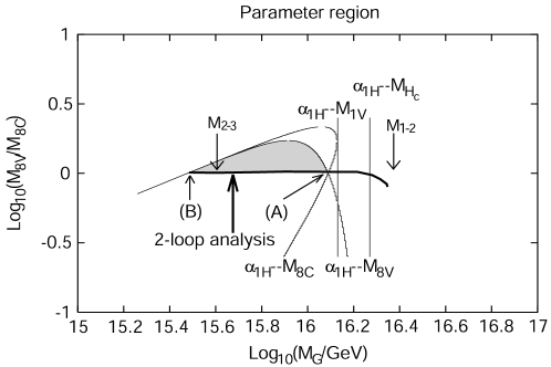
Figure 3: Parameter region of the SU(5)${}_{\rm GUT}\times$U(3)_H model. The parameter space of the model is spanned by three independent parameters: $M_{G}$, $M_{8V}/M_{8C}$ and $(M_{H_{c}}M_{H_{\bar{c}}})/M_{G}^{2}$. The figure is the $\sqrt{(M_{H_{c}}M_{H_{\bar{c}}})/M_{G}^{2}}=10^{0.3}$ cross section of the parameter space. We require that all the coupling constants remain finite under the renormalization group, while the renormalization point is below the heaviest particle of the model. This condition is satisfied in the shaded region when the 1-loop renormalization group is used. Thin curves and lines labelled “(gauge coupling)-mass” are lines where the corresponding gauge coupling constants become infinite at the corresponding mass scales. After two loop effects are included in the beta functions of the gauge coupling constants, the remaining allowed parameter region is only on the thick curve labelled 2-loop analysis. Points (A) and (B) denote the upper and the lower bound of the gauge-boson mass $M_{G}$, respectively, for fixed $\sqrt{(M_{H_{c}}M_{H_{\bar{c}}})/M_{G}^{2}}=10^{0.3}$. The upper bound of $M_{G}$ in the model is obtained as the maximum value $M_{G}$ takes at (A) as $\sqrt{(M_{H_{c}}M_{H_{\bar{c}}})/M_{G}^{2}}$ changes. One also sees immediately that the lower bound at (B) is so low that it is of no physical importance. $M_{1-2}$ ($M_{2-3}$) indicates the unification point between $1/\alpha_{1}$ and $1/\alpha_{2}$ ( $1/\alpha_{2}$ and $1/\alpha_{3}(-2\sigma)$ ) (see Fig. 1 for more details). Note that ($M_{G}$ at (A)) $<10^{16.13}$ GeV $\simeq$ (($0.60\simeq 10^{-0.22}$) $\times$ ($M_{1-2}\simeq 10^{16.35}$ GeV)). The QCD coupling constant $\alpha_{s}^{\overline{\rm MS},(5)}(M_{Z})=0.1132$ is used. The effects from a non-renormalizable operator that corresponds to (22) in this model are not included here.

The parameter region is shown in Fig. 3; only the $\sqrt{(M_{H_{c}}M_{H_{\bar{c}}}/M_{G}^{2})}=10^{0.3}$ cross section is described, and hence the region is described in the $M_{G}$–$(M_{8V}/M_{8C})$ plane. This analysis is based on the value of $\alpha_{3}(\mu)$ that is calculated from $\alpha^{\overline{\rm MS},(5)}_{s}(M_{Z})=0.1132$, i.e. a value smaller than the central value by 2$\sigma$. This is because it makes our analysis more conservative. The parameter region obtained by the 1-loop renormalization group is shown as the shaded area in Fig. 3. The region is bounded from the right and from the left, which is again consistent with the rough estimate of the matching scale given in subsection 2.3. The region is also bounded from below just for the same reason as in subsection 3.2. The parameter region distant from the (${\cal N}$ = 2)-SUSY line $M_{8V}\simeq M_{8C}$ is excluded when 2-loop effects are included in the beta functions of the gauge coupling constants; the 2-loop contributions have significant effects compared with 1-loop effects, because the 1-loop beta function of $\alpha_{\rm 3H}$ accidentally vanishes. The 1-loop renormalization-group evolution is reliable on the (${\cal N}$ = 2)-SUSY line, the thick line in Fig. 3, and hence the points indicated by (A) and (B) give the upper and the lower bound of $M_{G}$, respectively, in the $\sqrt{(M_{H_{c}}M_{H_{\bar{c}}}/M_{G}^{2})}=10^{0.3}$ cross section. The upper and the lower bound of $M_{G}$ of the model are the maximum and the minimum value that $M_{G}$ takes at (A) and (B), respectively, when the remaining parameter $(M_{H_{c}}M_{H_{\bar{c}}}/M_{G}^{2})$ is varied. Since it is evident from the figure that the lower bound of $M_{G}$ leads to too fast a proton decay, we focus in the following only on the upper bound of $M_{G}$.

4.2 Uncertainties in the Upper Bound of the Gauge-Boson Mass

In this subsection, we estimate uncertainties in the prediction of the upper bound of the GUT-gauge-boson mass obtained in the previous subsection. The uncertainties that originate from low-energy physics, however, are discussed in section 5.

First, we discuss the effects of the interactions that violate the ${\cal N}$ = 2 SUSY. The SU(5)_GUT gauge interaction and the cubic couplings in the fourth line of (2.2) are the sources of the violation of the ${\cal N}$ = 2 SUSY. Those interactions change the 1-loop-exact evolution of ${\cal N}$ = 2 SUSY gauge theories. The change in the upper bound of $M_{G}$ comes from the change in the evolution of $\alpha_{\rm 1H}$, because the upper bound was determined by the running of $\alpha_{\rm 1H}$ in the absence of (${\cal N}$ = 2)-SUSY breaking. The beta function of $\alpha_{\rm 1H}$ is changed at most by a few per cent, which leads to the change of the upper bound of $M_{G}$ by a factor of at most $10^{\pm 0.01}$.

Second, one can see from the matching equations [21] of this model that the gauge coupling constants $\alpha_{\rm 3H}$ and $\alpha_{\rm 1H}$ are not so large as to invalidate the perturbative expansion when the coloured-Higgs particles are moderately heavier than the GUT-gauge-boson mass; only one threshold correction from the coloured-Higgs particles is sufficient to keep both coupling constants within the perturbative regime. Non-perturbative effects are not important at all in such a region.

Finally, a non-renormalizable operator that corresponds to (22) may also exist in this model. Such an operator, if it exists, contributes to the matching equations at tree level. In its presence, we can perform exactly the same analysis as in the previous subsection. The result of this analysis is presented in section 6.

5 Conservative Upper Bound of Proton Lifetime

The analysis in sections 3 and 4 presented the way of extracting the upper bound of the GUT-gauge-boson mass for both models. The lifetime of the proton through the GUT-gauge-boson exchange is given [23] in terms of $M_{G}$ as

$$\tau(p\rightarrow\pi^{0}e^{+})\simeq 1.0\times 10^{35}\times\left(\frac{0.015{\rm GeV}^{3}}{\alpha_{\rm H}}\right)^{2}\left(\frac{2.5}{A_{R}}\right)^{2}\left(\frac{1}{25\alpha_{\rm GUT}(M_{G})}\right)^{2}\left(\frac{M_{G}}{10^{16}{\rm GeV}}\right)^{4}{\rm yrs},$$ (26)

where $\alpha_{\rm H}$ is a hadron matrix element calculated with lattice quenched QCD [30] ($\alpha_{\rm H}=-0.015\pm 0.001$ GeV³) renormalized at 2.3 GeV and $A_{R}\simeq 2.5$ a renormalization factor of the dimension-six proton-decay operators [31]; $A_{R}$ consists of a short-distance part, $A_{R}^{(\rm SD)}\simeq 2.1$, which comes from the renormalization between the GUT scale and the electroweak scale, and a long-distance part, $A_{R}^{(\rm LD)}\simeq 1.2$, from the renormalization between the electroweak scale and 2.3 GeV ($A_{R}=A_{R}^{(\rm SD)}\cdot A_{R}^{(\rm LD)}$). We note the expression of $A_{R}^{(\rm SD)}$ [32] for later convenience:

$$A_{R}^{(\rm SD)}=\left(\frac{\alpha_{C}(M_{Z})}{\alpha_{C}(M_{G})}\right)^{\frac{4/3}{b_{3}=3}}\left(\frac{\alpha_{L}(M_{Z})}{\alpha_{L}(M_{G})}\right)^{\frac{3/2}{b_{2}=-1}}\left(\frac{\alpha_{Y}(M_{Z})}{\alpha_{Y}(M_{G})}\right)^{\frac{23/30}{b_{1}=-33/5}},$$ (28)

where $b_{i}$ ($i=1,2,3$) are coefficients of the 1-loop beta functions of the three gauge coupling constants of the MSSM. The renormalization from Yukawa coupling constants is omitted because its effect is negligible.

Threshold corrections from SUSY particles are of the same order as those from the particles around the GUT scale. The 2-loop effects in the renormalization-group evolution between the electroweak scale and the GUT scale are also of the same order. Therefore, the two above effects should be taken into consideration in deriving predictions on the GUT-gauge-boson mass (and hence on the lifetime of the proton). This implies, in particular, that the predictions depend on the spectrum of SUSY particles. We present the predictions on the upper bound of the lifetime of the proton as a function of SUSY-breaking parameters of the mSUGRA boundary condition in subsection 5.1. Predictions can be obtained also for other SUSY-particle spectra such as that of gauge-mediated SUSY breaking (subsection 5.2). Subsection 5.3 discusses how the predictions are changed when there are vector-like SU(5)_GUT-multiplets at a scale below the GUT scale.

5.1 mSUGRA SUSY Threshold Corrections

Let us first consider the SUSY-particle spectrum determined by the mSUGRA boundary condition. This spectrum and the MSSM gauge coupling constants in the $\overline{{\rm DR}}$ scheme are calculated in an iterative procedure. We use the SOFTSUSY1.7 code [33] for this purpose. These coupling constants are evolved up to the GUT scale through the 2-loop renormalization group. They are used as input in the left-hand sides of, say, Eqs. (11)–(13), to obtain a prediction of the upper bound of the GUT-gauge-boson mass. The universal scalar mass $m_{0}$ and the universal gaugino mass $m_{1/2}$ are varied, while we fix the other parameters of the mSUGRA boundary condition; $\tan\beta=10.0$, $A_{0}=0$ GeV, and the sign of the $\mu$ parameter is the standard one.

The left panel of Fig. 4 is a contour plot on the $m_{0}$–$m_{1/2}$ plane, describing the upper bound of the proton lifetime in the SU(5)${}_{\rm GUT}\times$U(2)_H model, where we set the unknown coefficient $c$ of the non-renormalizable operator (22) to zero. The QCD coupling constant $\alpha_{s}^{\rm\overline{MS},(5)}(M_{Z})=0.1212$ is used, so that the upper bound becomes more conservative. One can see that this upper bound ranges over (1.4–3.2)$\times 10^{33}$ yrs. Notice that the ($m_{0}$, $m_{1/2}$) dependence of the proton lifetime arises almost only through the variation of $M_{2-3}$ (see Eq. (19)). Indeed, the contours of the upper bound of the lifetime in the left panel of Fig. 4 behave in the same way as those of $M_{2-3}$ in the upper-left panel of Fig. 5.

It is now easy to see how much the prediction is changed when we adopt the central value of the QCD coupling constant, $\alpha_{s}^{\rm\overline{MS},(5)}(M_{Z})=0.1172$. Since the choice of the QCD coupling constant directly changes $M_{2-3}$, it severely affects the upper bound of $M_{G}$ in this model. $M_{2-3}$ is decreased by a factor $e^{-\frac{2\pi}{b_{3}-b_{2}}(\frac{1}{0.1172}-\frac{1}{0.1212})}$, and the lifetime is shortened by a factor $e^{-2\pi\times 0.28}\simeq 0.2$. We confirmed that the upper bound of the lifetime does not exceed $1\times 10^{33}$ yrs even when the SUSY-breaking parameters $m_{0}$ and $m_{1/2}$ are varied up to 2000 GeV if we adopt the central value of the QCD coupling constant.

The hadron matrix element $\alpha_{\rm H}$ in [30], which has a statistical error $\alpha_{\rm H}=-0.015\pm 0.001{\rm GeV^{3}}$, does not include a systematic error (e.g. an error due to the quenched approximation). Reference [35] estimates that the systematic error is about 50%, which leads to an uncertainty in the lifetime of a factor of 2.

Therefore, the conservative upper bound is roughly $\tau\mathop{}_{\textstyle\sim}^{\textstyle<}6\times 10^{33}$ yrs, where we exploit the uncertainties in the SUSY threshold corrections, in the value of the QCD coupling constant and in the hadron matrix element. Thus, the prediction does not contradicts the experimental lower bound from Super-Kamiokande $\tau(p\rightarrow\pi^{0}e^{+})\mathop{}_{\textstyle\sim}^{\textstyle>}5\times 10^{33}$ yrs (90% C.L.) [36] at this moment, yet the large portion of the parameter region is already excluded. Moreover, one can expect that the uncertainties originating from low-energy physics will be reduced in the future. Thus, further accumulation of data in Super-Kamiokande and the next generation of water-Čerenkov detectors will be sure either to exclude this model without the non-renormalizable operator (22), or to detect the proton decay.

Now, we move to consider the SU(5)${}_{\rm GUT}\times$U(3)_H model. The right panel of Fig. 4 is a contour plot on the $m_{0}$–$m_{1/2}$ plane, describing the upper bound of the proton lifetime in the SU(5)${}_{\rm GUT}\times$U(3)_H model. The QCD coupling constant $\alpha_{s}^{\rm\overline{MS},(5)}(M_{Z})=0.1132$ is used. The upper bound of the proton lifetime ranges over (1–5)$\times 10^{35}$ yrs on the mSUGRA parameter space that is not excluded by the LEP II bound on the lightest-Higgs-boson mass.

Let us now see how much the above prediction is changed by uncertainties related to the QCD. First, the following observation is important in discussing the effect from the uncertainty in the value of the QCD coupling constant. The behaviour of the contours of the upper bound of the lifetime, and hence of the GUT-gauge-boson mass has, in this model, strong correlations with that of $M_{1-2}$ presented in the upper-right panel of Fig. 5. We find an empirical relation

$$M_{G}\mathop{}_{\textstyle\sim}^{\textstyle<}0.60\times M_{1-2}.$$ (29)

Thus, the upper bound does not depend on the value of the QCD coupling constant very much, since $M_{1-2}$ is not affected very much. Second, the uncertainty in the hadron form factor is common to both models. Therefore, the most conservative upper bound of the proton lifetime is roughly $\tau\mathop{}_{\textstyle\sim}^{\textstyle<}10^{36}$ yrs in this model. In particular, the proton decay might not be within the reach of the next generation of experiments.

5.2 Threshold Corrections from Various SUSY-Particle Spectrum

Gauge-mediated SUSY breaking (GMSB) is one of the highly motivated models of SUSY breaking. The spectrum of the SUSY particles is different from that of the mSUGRA SUSY breaking, and moreover, there are extra SU(5)_GUT-charged particles as messengers. Thus, the predictions on the proton lifetime are different from those in the case of mSUGRA SUSY breaking. We discuss the effects of the difference in the SUSY-particle spectra in this subsection. A possible change of predictions due to the existence of extra particles is discussed in the next subsection.

The ranges of the GUT-gauge-boson masses is different for different SUSY-particle spectra, yet the difference only arises from the difference in the two energy scales $M_{2-3}$ and $M_{1-2}$: the energy scale where the SU(2)_L and SU(3)_C coupling constants become the same and where those of U(1)_Y and SU(2)_L become the same, respectively. The upper bound of $M_{G}$ is given in terms of $M_{2-3}$ through Eq. (19) in the SU(5)${}_{\rm GUT}\times$U(2)_H model, and in terms of $M_{1-2}$ through Eq. (29) in the SU(5)${}_{\rm GUT}\times$U(3)_H model.

Figure 5 shows how $M_{2-3}$ and $M_{1-2}$ vary over the parameter space of the GMSB. The parameter space is spanned by two parameters: an overall mass scale $\Lambda$ of the SUSY breaking in the MSSM sector and the messenger mass $M_{\rm mess}$. We assume that the messenger sector consists of one pair of SU(5)_GUT-($\bf 5$+$\bf 5^{*}$) representations. Gaugino masses are given by

$$m_{\tilde{g}_{i}} = \frac{\alpha_{i}}{4\pi}\Lambda\left(1+{\cal O}\left(\frac{\Lambda}{M_{\rm mess}}\right)\right)\qquad(i=1,2,3)$$ (30)

at the threshold $M_{\rm mess}$. We calculate the SUSY-particle spectrum, the SUSY threshold corrections to the MSSM gauge coupling constants and the renormalization-group evolution to the messenger scale using the code [33]. We include contributions from the messenger particles into the beta functions in the renormalization-group evolution from the messenger scale to the GUT scale. $M_{2-3}$ and $M_{1-2}$ are obtained and are shown in Fig. 5. It is clear from Fig. 5 that the ranges of $M_{2-3}$ and $M_{1-2}$ are almost the same in the mSUGRA and GMSB parameter spaces. Therefore, we conclude that there is little effect that comes purely from the difference between the SUSY-particle spectra of the mSUGRA and GMSB.

The gaugino masses satisfy the GUT relation in both the mSUGRA and GMSB spectra, which may be the reason why $M_{2-3}$ and $M_{1-2}$ are almost the same in the two spectra. The gaugino mass spectrum, however, might not satisfy the GUT relation. Even in this case, we can obtain the upper bound of the lifetime through $M_{2-3}$ for the SU(5)${}_{\rm GUT}\times$U(2)_H model and through $M_{1-2}$ for the SU(5)${}_{\rm GUT}\times$U(3)_H model.

5.3 Vector-Like SU(5)_GUT-Multiplet at Low Energy

There are several motivations to consider charged particles in vector-like representations, whose masses are of the order of the SUSY-breaking scale or an intermediate scale. Messenger particles are necessary in the GMSB models, and the anomaly cancellation of the discrete R symmetry also requires [39] extra particles such as SU(5)_GUT-(5+5^∗).

There are three effects on the proton lifetime in the presence of these particles. The first two effects come from the change in the values of the unified coupling constant $\alpha_{\rm GUT}$ and the renormalization factor $A_{R}$ of the proton-decay operators. First, the unified gauge coupling constant is larger in the presence of new particles, and hence the decay rate is enhanced. Then, the lifetime is shortened by a factor not smaller than 0.66 when a vector-like pair SU(5)_GUT-(5+5^∗) exists at an energy scale not lower than 1 TeV. Second, the renormalization factor $A_{R}$ is changed by such a vector-like pair only in its short-distance part. The new expression for $A^{(\rm SD)}_{R}$ is now given by

$$A_{R}^{(\rm SD)} = \left(\frac{\alpha_{C}(M_{Z})}{\alpha_{C}(M)}\right)^{\frac{4/3}{3}}\left(\frac{\alpha_{L}(M_{Z})}{\alpha_{L}(M)}\right)^{\frac{3/2}{-1}}\left(\frac{\alpha_{Y}(M_{Z})}{\alpha_{Y}(M)}\right)^{\frac{23/30}{-33/5}}$$ (31)

$$\times\left(\frac{\alpha_{C}(M)}{\alpha_{C}(M_{G})}\right)^{\frac{4/3}{2}}\left(\frac{\alpha_{L}(M)}{\alpha_{L}(M_{G})}\right)^{\frac{3/2}{-2}}\left(\frac{\alpha_{Y}(M)}{\alpha_{Y}(M_{G})}\right)^{\frac{23/30}{-38/5}},$$

where $M$ is the mass scale of the vector-like pair. We find that $A_{R}^{(\rm SD)}$ increases from 2.1 to 2.5 as the mass scale $M$ decreases from the GUT scale to 1 TeV. Thus, the lifetime is shortened by a factor not smaller than 0.71 because of the renormalization factor.

The third effect is due to threshold corrections from the vector-like particles. The triplets and doublets in the vector-like pair 5+5^∗ are expected to have different masses, just as the bottom quark and tau lepton do. The triplets will be heavier than the doublets by

$$\frac{M_{{\bf 3}+{\bf 3}^{*}}}{M_{{\bf 2}+{\bf 2}^{*}}}\simeq\left(\frac{\alpha_{C}(M_{{\bf 5}+{\bf 5}^{*}})}{\alpha_{C}(M_{G})}\right)^{\frac{4}{3}},$$ (32)

which increases from 1.0 to 2.1 as the mass scale $M_{{\bf 5+5^{*}}}$ of a vector-like pair SU(5)_GUT-(5+5^∗) decreases from the GUT scale to 1 TeV. The upper bound of the proton lifetime in the SU(5)${}_{\rm GUT}\times$U(2)_H model becomes tighter by a factor $(M_{{\bf 2}+{\bf 2}^{*}}/M_{{\bf 3}+{\bf 3}^{*}})\mathop{}_{\textstyle\sim}^{\textstyle>}0.48$ as $M_{2-3}$ is decreased by a factor $(M_{{\bf 2}+{\bf 2}^{*}}/M_{{\bf 3}+{\bf 3}^{*}})^{1/4}$; in the SU(5)${}_{\rm GUT}\times$U(3)_H model, instead, it is loosened by a factor $(M_{{\bf 3}+{\bf 3}^{*}}/M_{{\bf 2}+{\bf 2}^{*}})^{2/7}\mathop{}_{\textstyle\sim}^{\textstyle<}1.2$ as $M_{1-2}$ is increased.

The proton decay is, thus, enhanced by all three effects in the SU(5)${}_{\rm GUT}\times$U(2)_H model; the lifetime is shortened by a factor of 0.22 when SU(5)_GUT-(5+5^∗) exists at 1 TeV. The rate is enhanced also in the SU(5)${}_{\rm GUT}\times$U(3)_H model; the lifetime is shortened by a factor of 0.56.

6 Conclusions and Discussion

We analysed the proton-decay amplitude in a class of models of SUSY GUTs: SU(5)_GUT $\times$U($N$)_H models with $N=2,3$. Dimension-five proton-decay operators are completely forbidden, and hence the gauge-boson exchange is the process that dominates the proton decay. We found that the gauge-boson mass is bounded from above by

$$M_{G}\mathop{}_{\textstyle\sim}^{\textstyle<}0.40\times 10^{-0.82\times c}\times M_{2-3}$$ (33)

in the SU(5)${}_{\rm GUT}\times$U(2)_H model and by

$$M_{G}\mathop{}_{\textstyle\sim}^{\textstyle<}0.60\times 10^{-0.4\times c}\times M_{1-2}$$ (34)

in the SU(5)${}_{\rm GUT}\times$U(3)_H model. Here, $M_{2-3}$ ($M_{1-2}$) denotes an energy scale where SU(2)_L and SU(3)_C (U(1)_Y and SU(2)_L) gauge coupling constants are equal, respectively. In the right-hand sides, $c$ are coefficients of non-renormalizable operator (22) in the SU(5)${}_{\rm GUT}\times$U(2)_H model and of the one that corresponds to (22) in the SU(5)${}_{\rm GUT}\times$U(3)_H model. It is quite important to note that the upper bound was obtained in these models (for fixed $c$), which leads to the upper bound of the lifetime. Although the gauge-boson masses are bounded also from below in the latter model, the lower bound is of no importance. This is because it predicts a lifetime much shorter than the lower bound obtained so far from experiments.

The coefficients $c$ directly affect the gauge coupling unification, and hence they appear in the above formulae. One will see later that they are the largest source of uncertainties in the upper bound of the lifetime if $c$ are of the order of unity. Although there may be an extra (broken) symmetry or any dynamics that suppress the non-renormalizable operators, we leave $c$ in the formulae for generic cases.

In section 1, we briefly mentioned two other classes of models of SUSY GUTs constructed in four-dimensional space-time. Let us make a brief summary on the mass of the gauge bosons of such models before we proceed to a discussion of the lifetime.

Let us first discuss the gauge-boson mass in the models in [10, 11]. The spectrum around the GUT scale consists of three ((adj.,1)⁰ + (1,adj)⁰)’s and two ((3,2)^-5/6 + h.c.)’s of the MSSM gauge group, in addition to the GUT gauge boson. Parameters of the models allow a spectrum where the matter particles are lighter than the GUT gauge boson. Then, 1-loop threshold corrections from such a spectrum imply that the GUT-gauge-boson mass is heavier than the energy scale of approximate unification [43]. Therefore, no upper bound is virtually obtained in the models in [10, 11]. A lower bound might be obtained, yet no full study has been done so far. Non-renormalizable operators in the gauge kinetic functions affect the matching equations just as in our analysis.

On the contrary, in the models in [18], non-renormalizable operators do not affect the matching equations and, moreover, the mass of the GUT gauge boson is smaller than the energy scale where the three gauge coupling constants are approximately unified:

$$M_{G}\sim\lambda^{a}M_{\rm unif},$$ (35)

where $M_{\rm unif}\sim M_{2-3}\sim M_{1-2}$, $\lambda$ a small parameter of the order of $10^{-1}$ and $a$ the charge of a field whose VEV breaks the SU(5)_GUT symmetry down to SU(3)${}_{C}\times$SU(2)${}_{L}\times$U(1)_Y. Thus, $M_{G}$ is fairly small in the models. The upper bound would be obtained once a model ($\lambda$ and $a$, in particular) is fixed. The Super-Kamiokande experiment already puts constraints on the choice of $\lambda$ and $a$. The proton decays also through dimension-five operators, although these operators can be suppressed in some models in this class.

Thus, the ranges of the proton lifetime of those models lie in the following order:

$$\tau(\cite[cite]{[\@@bibref{}{Maekawa}{}{}]})_{\rm dim.6}\sim\tau(\mathop{\rm SU}(5)_{\rm GUT}\times\mathop{\rm U}(2)_{\rm H})\mathop{}_{\textstyle\sim}^{\textstyle<}\tau(\mathop{\rm SU}(5)_{\rm GUT}\times\mathop{\rm U}(3)_{\rm H})\mathop{}_{\textstyle\sim}^{\textstyle<}\tau(\cite[cite]{[\@@bibref{}{BDS}{}{}]},\cite[cite]{[\@@bibref{}{Barr}{}{}]}).$$ (36)

However, the ranges would have certain amount of overlap between one another, and hence it would be impossible to single out a model only from the decay rate of the proton. Detailed information on the branching ratio of various decay modes does not help for that purpose either; the decay is induced in all the above models by one and the same mechanism: the gauge-boson exchange.

Even if no model can be singled out, one can, and one will be able to exclude some of the models on the basis of experimental results currently available and obtained in the future, respectively. We summarize, in the following, the upper bound of the proton lifetime for the SU(5)${}_{\rm GUT}\times$U(2)_H model and the SU(5)${}_{\rm GUT}\times$U(3)_H model. It would also be of importance if one finds an upper bound and a lower bound of the lifetime in models in [18] and in [10, 11, 12], respectively.

Now the proton lifetime is bounded from above by

$$\tau(p\rightarrow\pi^{0}e^{+})\mathop{}_{\textstyle\sim}^{\textstyle<}4.1\times 10^{32}\left(\frac{M_{2-3}}{10^{15.8}{\rm GeV}}\right)^{4}\left(10^{-3.2c}\right)\left(\frac{0.015{\rm GeV}^{3}}{\alpha_{\rm H}}\right)^{2}\left(\frac{1}{25\alpha_{\rm GUT}}\right)^{2}\left(\frac{2.5}{A_{R}}\right)^{2}{\rm yrs}$$ (37)

in the SU(5)${}_{\rm GUT}\times$U(2)_H model. The largest uncertainty in this prediction comes from the value of $c$. Another from the systematic error in $\alpha_{\rm H}$. No estimate is available for the value of $c$. The error in $\alpha_{\rm H}$ is not studied very much, yet the lifetime is changed by a factor of (0.5–2) if the conservative estimate in [35] is adopted. The experimental value of the QCD coupling constant $\alpha_{s}^{\overline{\rm MS},(5)}(M_{Z})$ changes the prediction through the change in $M_{2-3}$. The upper bound is changed by a factor of (0.15–5.9) when the coupling constant is varied by $\pm 2\sigma$ error determined by experiments. The threshold corrections from SUSY particles also changes the prediction through the change in $M_{2-3}$. They change $M_{2-3}$ typically from $10^{15.77}$ GeV to $10^{15.90}$ GeV, and hence the upper bound is changed by a factor of (0.75–2.5). Therefore, the theoretical upper bound exceeds the experimental lower bound ($\tau(p\rightarrow\pi^{0}e^{+})\mathop{}_{\textstyle\sim}^{\textstyle>}5\times 10^{33}$ yrs; 90% C.L.) only when all the low-energy uncertainties are exploited. See section 3.3 for the uncertainties that arise in the way of our analysis.

The lifetime is shortened by a factor not smaller than 0.22 if SU(5)_GUT-(5+5^∗) exists at low energy. The threshold corrections from these particles contribute by a factor not smaller than 0.47 through the change in $M_{2-3}$, and the changes in $\alpha_{\rm GUT}$ and in $A_{R}$ contribute by factors not smaller than 0.66 and 0.71, respectively. Thus, those particles at 1 TeV would hardly be reconciled with the experimetal bound without incorporating the non-renormalizable operator (22).

The lifetime is bounded from above by

$$\tau(p\rightarrow\pi^{0}e^{+})\mathop{}_{\textstyle\sim}^{\textstyle<}2.1\times 10^{35}\left(\frac{M_{1-2}}{10^{16.3}{\rm GeV}}\right)^{4}\left(10^{-2c}\right)\left(\frac{0.015{\rm GeV}^{3}}{\alpha_{\rm H}}\right)^{2}\left(\frac{1}{25\alpha_{\rm GUT}}\right)^{2}\left(\frac{2.5}{A_{R}}\right)^{2}{\rm yrs}$$ (38)

in the SU(5)${}_{\rm GUT}\times$U(3)_H model. Uncertainties arise from $c$ and $\alpha_{\rm H}$ as in the previous model. The value of the QCD coupling constant is not relevant to the prediction. The SUSY threshold corrections changes the upper bound typically by a factor of (0.40–2.5) as $M_{1-2}$ changes from $10^{16.20}$ GeV to $10^{16.40}$ GeV.

The lifetime is shortened by a factor not smaller than 0.56 in the presence of SU(5)_GUT-(5+5^∗) below the GUT scale. The decay is more enhanced as their mass is smaller. The enhancement factor 0.56 (when the mass is 1 TeV) consists of suppression factor 1.2, which comes from $M_{1-2}$ changed by threshold corrections of these particles, and enhancement factors 0.66 and 0.71 respectively from $\alpha_{\rm GUT}$ and $A_{R}$.

Appendix A Renormalization-Group Equations

In this section, renormalization-group equations of coupling constants of the models are listed.

SU(5)${}_{\rm GUT}\times$U(2)_H model

$$\frac{\partial}{\partial\ln\mu}\left(\frac{1}{\alpha_{\rm 2H}}(\mu)\right) = \frac{-2}{2\pi}\qquad\qquad\qquad\mbox{(1-loop)}$$

$$- \frac{2}{2\pi}\frac{(6\alpha_{\rm 2H}-5\alpha_{\rm 2H}^{\lambda}-\alpha_{\rm 2H}^{\lambda^{\prime}})}{2\pi}$$

$$- \frac{1}{2\pi}\frac{6(3\alpha_{\rm 2H}+\alpha_{\rm 1H})-5(3\alpha_{\rm 2H}^{\lambda}+\alpha_{\rm 1H}^{\lambda})-(3\alpha_{\rm 2H}^{\lambda^{\prime}}+\alpha_{\rm 1H}^{\lambda^{\prime}})}{4\pi}$$

$$-\frac{5}{2\pi}\left(\frac{\frac{24}{10}}{\pi}\alpha_{\rm GUT}\right).$$

$$\frac{\partial}{\partial\ln\mu}\left(\frac{1}{\alpha_{\rm 2H}^{\lambda}}(\mu)\right) = \frac{-2}{2\pi}\left(\frac{\alpha_{\rm 2H}}{\alpha_{\rm 2H}^{\lambda}}\right)+\frac{1}{\alpha_{\rm 2H}^{\lambda}}\frac{(6\alpha_{\rm 2H}-5\alpha_{\rm 2H}^{\lambda}-\alpha_{\rm 2H}^{\lambda^{\prime}})}{2\pi}$$

$$+ \frac{2}{\alpha_{\rm 2H}^{\lambda}}\frac{(3\alpha_{\rm 2H}+\alpha_{\rm 1H})-(3\alpha_{\rm 2H}^{\lambda}+\alpha_{\rm 1H}^{\lambda})}{4\pi}$$

$$+\frac{2}{\alpha_{\rm 2H}^{\lambda}}\left(\frac{\frac{24}{10}}{\pi}\alpha_{\rm GUT}\right).$$

$$\frac{\partial}{\partial\ln\mu}\left(\frac{1}{\alpha_{\rm 2H}^{\lambda^{\prime}}}(\mu)\right) = \frac{-2}{2\pi}\left(\frac{\alpha_{\rm 2H}}{\alpha_{\rm 2H}^{\lambda^{\prime}}}\right)+\frac{1}{\alpha_{\rm 2H}^{\lambda^{\prime}}}\frac{(6\alpha_{\rm 2H}-5\alpha_{\rm 2H}^{\lambda}-\alpha_{\rm 2H}^{\lambda^{\prime}})}{2\pi}$$

$$+ \frac{2}{\alpha_{\rm 2H}^{\lambda^{\prime}}}\frac{(3\alpha_{\rm 2H}+\alpha_{\rm 1H})-(3\alpha_{\rm 2H}^{\lambda^{\prime}}+\alpha_{\rm 1H}^{\lambda^{\prime}})}{4\pi}.$$

$$\frac{\partial}{\partial\ln\mu}\left(\frac{1}{\alpha_{\rm 1H}}(\mu)\right) = \frac{-6}{2\pi}\qquad\qquad\qquad\mbox{(1-loop)}$$

$$- \frac{1}{2\pi}\frac{6(3\alpha_{\rm 2H}+\alpha_{\rm 1H})-5(3\alpha_{\rm 2H}^{\lambda}+\alpha_{\rm 1H}^{\lambda})-(3\alpha_{\rm 2H}^{\lambda^{\prime}}+\alpha_{\rm 1H}^{\lambda^{\prime}})}{4\pi}$$

$$-\frac{5}{2\pi}\left(\frac{\frac{24}{10}}{\pi}\alpha_{\rm GUT}\right).$$

$$\frac{\partial}{\partial\ln\mu}\left(\frac{1}{\alpha_{\rm 1H}^{\lambda}}(\mu)\right) = \frac{-6}{2\pi}\left(\frac{\alpha_{\rm 1H}}{\alpha_{\rm 1H}^{\lambda}}\right)+\frac{1}{\alpha_{\rm 1H}^{\lambda}}\frac{(6\alpha_{\rm 1H}-5\alpha_{\rm 1H}^{\lambda}-\alpha_{\rm 1H}^{\lambda^{\prime}})}{2\pi}$$

$$+ \frac{2}{\alpha_{\rm 1H}^{\lambda}}\frac{(3\alpha_{\rm 2H}+\alpha_{\rm 1H})-(3\alpha_{\rm 2H}^{\lambda}+\alpha_{\rm 1H}^{\lambda})}{4\pi}$$

$$+\frac{2}{\alpha_{\rm 1H}^{\lambda}}\left(\frac{\frac{24}{10}}{\pi}\alpha_{\rm GUT}\right).$$

$$\frac{\partial}{\partial\ln\mu}\left(\frac{1}{\alpha_{\rm 1H}^{\lambda^{\prime}}}(\mu)\right) = \frac{-6}{2\pi}\left(\frac{\alpha_{\rm 1H}}{\alpha_{\rm 1H}^{\lambda^{\prime}}}\right)+\frac{1}{\alpha_{\rm 1H}^{\lambda^{\prime}}}\frac{(6\alpha_{\rm 1H}-5\alpha_{\rm 1H}^{\lambda}-\alpha_{\rm 1H}^{\lambda^{\prime}})}{2\pi}$$

$$+ \frac{2}{\alpha_{\rm 1H}^{\lambda^{\prime}}}\frac{(3\alpha_{\rm 2H}+\alpha_{\rm 1H})-(3\alpha_{\rm 2H}^{\lambda^{\prime}}+\alpha_{\rm 1H}^{\lambda^{\prime}})}{4\pi}.$$

SU(5)${}_{\rm GUT}\times$U(3)_H model

$$\frac{\partial}{\partial\ln\mu}\left(\frac{1}{\alpha_{\rm 3H}}(\mu)\right) = 0\qquad\qquad\qquad\mbox{(1-loop)}$$

$$- \frac{3}{2\pi}\frac{(6\alpha_{\rm 3H}-5\alpha_{\rm 3H}^{\lambda}-\alpha_{\rm 3H}^{\lambda^{\prime}})}{2\pi}$$

$$- \frac{1}{2\pi}\frac{6(8\alpha_{\rm 3H}+\alpha_{\rm 1H})-5(8\alpha_{\rm 3H}^{\lambda}+\alpha_{\rm 1H}^{\lambda})-(8\alpha_{\rm 3H}^{\lambda^{\prime}}+\alpha_{\rm 1H}^{\lambda^{\prime}})}{6\pi}$$

$$+\left(-\frac{5}{2\pi}\frac{\frac{24}{10}}{\pi}\alpha_{\rm GUT}+\frac{10}{2\pi}\frac{1}{2\pi}\alpha_{h}\right).$$

$$\frac{\partial}{\partial\ln\mu}\left(\frac{1}{\alpha_{\rm 3H}^{\lambda}}(\mu)\right) = 0+\frac{1}{\alpha_{\rm 3H}^{\lambda}}\frac{(6\alpha_{\rm 3H}-5\alpha_{\rm 3H}^{\lambda}-\alpha_{\rm 3H}^{\lambda^{\prime}})}{2\pi}$$

$$+ \frac{2}{\alpha_{\rm 3H}^{\lambda}}\frac{(8\alpha_{\rm 3H}+\alpha_{\rm 1H})-(8\alpha_{\rm 3H}^{\lambda}+\alpha_{\rm 1H}^{\lambda})}{6\pi}$$

$$+\frac{2}{\alpha_{\rm 3H}^{\lambda}}\left(\frac{\frac{24}{10}}{\pi}\alpha_{\rm GUT}-\frac{1}{2\pi}\alpha_{h}\right).$$

$$\frac{\partial}{\partial\ln\mu}\left(\frac{1}{\alpha_{\rm 3H}^{\lambda^{\prime}}}(\mu)\right) = 0+\frac{1}{\alpha_{\rm 3H}^{\lambda^{\prime}}}\frac{(6\alpha_{\rm 3H}-5\alpha_{\rm 3H}^{\lambda}-\alpha_{\rm 3H}^{\lambda^{\prime}})}{2\pi}$$

$$+ \frac{2}{\alpha_{\rm 3H}^{\lambda^{\prime}}}\frac{(8\alpha_{\rm 3H}+\alpha_{\rm 1H})-(8\alpha_{\rm 3H}^{\lambda^{\prime}}+\alpha_{\rm 1H}^{\lambda^{\prime}})}{6\pi}$$

$$+\frac{2}{\alpha_{\rm 3H}^{\lambda^{\prime}}}\left(\qquad\qquad\qquad-\frac{5}{2\pi}\alpha_{h}\right).$$

$$\frac{\partial}{\partial\ln\mu}\left(\frac{1}{\alpha_{\rm 1H}}(\mu)\right) = \frac{-6}{2\pi}\qquad\qquad\qquad\mbox{(1-loop)}$$

$$- \frac{1}{2\pi}\frac{6(8\alpha_{\rm 3H}+\alpha_{\rm 1H})-5(8\alpha_{\rm 3H}^{\lambda}+\alpha_{\rm 1H}^{\lambda})-(8\alpha_{\rm 3H}^{\lambda^{\prime}}+\alpha_{\rm 1H}^{\lambda^{\prime}})}{6\pi}$$

$$+\left(-\frac{5}{2\pi}\frac{\frac{24}{10}}{\pi}\alpha_{\rm GUT}+\frac{10}{2\pi}\frac{1}{2\pi}\alpha_{h}\right).$$

$$\frac{\partial}{\partial\ln\mu}\left(\frac{1}{\alpha_{\rm 1H}^{\lambda}}(\mu)\right) = \frac{-6}{2\pi}\left(\frac{\alpha_{\rm 1H}}{\alpha_{\rm 1H}^{\lambda}}\right)+\frac{1}{\alpha_{\rm 1H}^{\lambda}}\frac{(6\alpha_{\rm 1H}-5\alpha_{\rm 1H}^{\lambda}-\alpha_{\rm 1H}^{\lambda^{\prime}})}{2\pi}$$

$$+ \frac{2}{\alpha_{\rm 1H}^{\lambda}}\frac{(8\alpha_{\rm 3H}+\alpha_{\rm 1H})-(8\alpha_{\rm 3H}^{\lambda}+\alpha_{\rm 1H}^{\lambda})}{6\pi}$$

$$+\frac{2}{\alpha_{\rm 1H}^{\lambda}}\left(\frac{\frac{24}{10}}{\pi}\alpha_{\rm GUT}-\frac{1}{2\pi}\alpha_{h}\right).$$

$$\frac{\partial}{\partial\ln\mu}\left(\frac{1}{\alpha_{\rm 1H}^{\lambda^{\prime}}}(\mu)\right) = \frac{-6}{2\pi}\left(\frac{\alpha_{\rm 1H}}{\alpha_{\rm 1H}^{\lambda^{\prime}}}\right)+\frac{1}{\alpha_{\rm 1H}^{\lambda^{\prime}}}\frac{(6\alpha_{\rm 1H}-5\alpha_{\rm 1H}^{\lambda}-\alpha_{\rm 1H}^{\lambda^{\prime}})}{2\pi}$$

$$+ \frac{2}{\alpha_{\rm 1H}^{\lambda^{\prime}}}\frac{(8\alpha_{\rm 3H}+\alpha_{\rm 1H})-(8\alpha_{\rm 3H}^{\lambda^{\prime}}+\alpha_{\rm 1H}^{\lambda^{\prime}})}{6\pi}$$

$$+\frac{2}{\alpha_{\rm 1H}^{\lambda^{\prime}}}\left(\qquad\qquad\qquad-\frac{5}{2\pi}\alpha_{h}\right).$$

$$\frac{\partial}{\partial\ln\mu}\left(\frac{1}{\alpha_{h}}(\mu)\right) = \frac{1}{\alpha_{h}}\frac{2(8\alpha_{\rm 3H}+\alpha_{\rm 1H})-(8\alpha_{\rm 3H}^{\lambda}+\alpha_{\rm 1H}^{\lambda})-(8\alpha_{\rm 3H}^{\lambda^{\prime}}+\alpha_{\rm 1H}^{\lambda^{\prime}})}{6\pi}$$

$$+\left(\frac{1}{\alpha_{h}}\right)\left(\frac{2\times\frac{24}{10}}{\pi}\alpha_{\rm GUT}-\frac{(1+5+3)}{2\pi}\alpha_{h}\right).$$

Appendix B ${\cal N}$ = 2 SUSY and Infrared-Fixed
Renormalization-Group Flow

Particle contents in the GUT-symmetry-breaking sector of the SU(5)${}_{\rm GUT}\times$U(2)_H model can be regarded as multiplets of the ${\cal N}$ = 2 SUSY [17], and ${\cal N}$ = 2 SUSY is enhanced in this sector [8] when the SU(5)_GUT gauge interaction is neglected and coupling constants satisfy

$$g_{\rm 1H}\simeq\lambda_{\rm 1H}(\sim\lambda_{\rm 1H}^{\prime}),\qquad\qquad g_{\rm 2H}\simeq\lambda_{\rm 2H}(\sim\lambda_{\rm 2H}^{\prime}).$$ (52)

One can see in the right panel of Fig. 2 that the parameter region survives in the presence of the 2-loop effects only when the ${\cal N}$ = 2 SUSY is approximately preserved; the $M_{3V}\simeq M_{3C}$ line is equivalent to $\alpha_{\rm 2H}\simeq\alpha_{\rm 2H}^{\lambda^{(^{\prime})}}$ when the SU(5)_GUT gauge interaction is neglected.

This is not a coincidence. In any gauge theory with ${\cal N}$ = 2 SUSY, gauge coupling constants are renormalized only at the 1-loop level [26]. Anomalous dimensions of hypermultiplets vanish [28] at all orders in perturbative expansion, and even non-perturbatively. Therefore, the parameter allowed in the 1-loop analysis is still allowed when ${\cal N}$ = 2 SUSY is preserved even after the 2-loop effects have also been taken into account.

The band of the region around the (${\cal N}$ = 2)-SUSY line almost becomes a line as $M_{G}$ becomes larger. For parameters above that line, the $\alpha_{\rm 2H}$ coupling constant becomes large at a renormalization point lower than $M_{3V}$, while for parameters below the line, the $\alpha_{\rm 2H}^{\lambda}$ coupling becomes large at a renormalization point lower than $M_{3C}$; a viable set of parameters was not found for large $M_{G}$ even on the line in our numerical calculation. It does not mean, however, that the parameter does not exist at all on the (${\cal N}$ = 2)-SUSY line ($M_{3V}\simeq M_{3C}$) for large $M_{G}$, as seen below. The (${\cal N}$ = 2)-SUSY relations (52) are not only renormalization-group invariant but also infrared (IR)-fixed relations of the renormalization group:

$$\frac{\partial}{\partial\ln\mu}\left(\frac{1}{\alpha_{\rm 2H}}-\frac{1}{\alpha_{\rm 2H}^{\lambda}}\right)(\mu) = \left(\frac{21}{2\pi}+\frac{7}{\alpha_{\rm 2H}^{\lambda}}\right)\frac{(\alpha_{\rm 2H}^{\lambda}-\alpha_{\rm 2H})}{2\pi}+\left(\frac{6}{2\pi}+\frac{2}{\alpha_{\rm 2H}^{\lambda}}\right)\frac{(\alpha_{\rm 1H}^{\lambda}-\alpha_{\rm 1H})}{4\pi},$$ (53)

$$\frac{\partial}{\partial\ln\mu}\left(\frac{1}{\alpha_{\rm 1H}}-\frac{1}{\alpha_{\rm 1H}^{\lambda}}\right)(\mu) = \left(\frac{6}{2\pi}+\frac{2}{\alpha_{\rm 1H}^{\lambda}}\right)\frac{3(\alpha_{\rm 2H}^{\lambda}-\alpha_{\rm 2H})+(\alpha_{\rm 1H}^{\lambda}-\alpha_{\rm 1H})}{4\pi},$$ (54)

where the SU(5)_GUT interaction is still neglected. This implies that the renormalization-group evolution to UV immediately becomes unstable, even for a set of parameters that is slightly distant from the IR-fixed relations. The IR-fixed property (UV instability) also implies that the parameter region is thin only when $M=M_{G}$, and not when the coupling constants are evaluated at $M\gg M_{G}$.

Thus, we can expect that the 1-loop analysis is completely reliable for a set of parameters exactly on the (${\cal N}=2$)-SUSY line and, in particular, that a viable set of parameters does exist on the line even if it is not found in the numerical analysis. Therefore, the maximum value of $M_{G}$ is given at a point indicated by an arrow in the right panel of Fig. 2. At least, there would be no doubt that the maximum value of $M_{G}$ obtained in such a way provides a conservative upper bound of $M_{G}$.

The above argument, however, is correct only when the SU(5)_GUT gauge interaction is neglected. Therefore, let us now discuss the effects of the SU(5)_GUT gauge interaction. These break the ${\cal N}$ = 2 SUSY in the sector. Thus, the (${\cal N}$ = 2)-SUSY relations in Eq. (52) are no longer renormalization-group-invariant, and the renormalization-group flow is no longer 1-loop exact. However, the SU(5)_GUT interaction is much weaker than the U(2)_H interactions, and its effects are small. Thus, they can be treated as small perturbations to the (${\cal N}$ = 2)-SUSY flow. In particular, the IR-fixed property of the renormalization-group equations (A)–(A) is not changed, except that the IR-fixed relations are slightly modified into

$$(\alpha_{\rm 2H}-\alpha_{\rm 2H}^{\lambda}),\;\;(\alpha_{\rm 2H}-\alpha_{\rm 2H}^{\lambda^{\prime}}),\;\;(\alpha_{\rm 1H}-\alpha_{\rm 1H}^{\lambda}),\;\;(\alpha_{\rm 1H}-\alpha_{\rm 1H}^{\lambda^{\prime}})\simeq{\cal O}(\alpha_{\rm GUT}).$$ (55)

Coupling constants flow down into the modified fixed relations and then follow the relations. Thus, the evolution of the coupling constants toward the UV is the most stable when the parameter satisfies the “IR-fixed relations”. The modified fixed relations are still almost the (${\cal N}$ = 2)-SUSY relations, and hence the 1-loop evolution is almost correct for the parameter satisfying the relations; beta functions are different from those at one loop only by an order of $\alpha_{\rm GUT}$. Moreover, combinations such as $(\alpha_{\rm 2H}$ – $\alpha_{\rm 2H}^{\lambda^{(^{\prime})}})$ partially absorb the SU(5)_GUT contributions in the beta functions. Therefore, the corrections to the 1-loop evolution are estimated conservatively from above when the SU(5)_GUT contribution is purely added to the 1-loop beta functions, as we did in subsection 3.3.

Fields	${\bf 10}^{ij}$	${\bf 5}^{*}_{i}$	$X$	$Q_{i},\bar{Q}^{i}$	$Q_{6}$,$\bar{Q}^{6}$
R charges	1	1	2	0	0

Table 1: (Mod 4)-R charges of the fields in the SU(5)${}_{\rm GUT}\times$U(2)_H model.

Fields	${\bf 10}^{ij}$	${\bf 5}^{*}_{i}$	$H({\bf 5})^{i}$	$\bar{H}({\bf 5}^{*})_{i}$	$X^{\alpha}_{\;\;\beta}$	$Q^{\alpha}_{\;\;i}$	$\bar{Q}^{i}_{\;\;\alpha}$	$Q^{\alpha}_{6}$	$\bar{Q}^{6}_{\;\;\alpha}$
R charges	1	1	0	0	2	$0$	$0$	$2$	$-2$

Table 2: (Mod 4)-R charges of the fields in the SU(5)${}_{\rm GUT}\times$U(3)_H model.

(3,2)${}^{-\frac{5}{6}}$	(1,1)0	(1,1)0	(1,adj.)0	(1,adj.)0
m.vect.	m.vect.	$\chi+\chi^{\dagger}$	m.vect.	$\chi+\chi^{\dagger}$
$M_{G}=$	$M_{1V}=$	$M_{1C}=$	$M_{3V}=$	$M_{3C}=$
$\sqrt{2}g_{\rm GUT}v$	$\sqrt{2(g_{\rm 1H}^{2}+3g_{\rm GUT}^{2}/5)}v$	$\sqrt{2}\lambda_{\rm 1H}v$	$\sqrt{2(g_{\rm 2H}^{2}+g_{\rm GUT}^{2})}v$	$\sqrt{2}\lambda_{\rm 2H}v$

Table 3: Summary of the particle spectrum around the GUT scale of the SU(5)${}_{\rm GUT}\times$U(2)_H model. The first line denotes the representation under the gauge group of the MSSM. In the second line, m.vect. denotes ${\cal N}$ = 1 massive vector multiplets and $\chi+\chi^{\dagger}$ a pair of ${\cal N}$ = 1 chiral and antichiral multiplets. In the last line, the mass of each multiplet are given in terms of gauge coupling constants and parameters in the superpotential (2.1).

(${\bf 3},{\bf 2})^{-\frac{5}{6}}$	$({\bf 3},{\bf 1})^{-\frac{1}{3}}$	$({\bf 3},{\bf 1})^{-\frac{1}{3}}$	$({\bf 1},{\bf 1})^{0}$	$({\bf 1},{\bf 1})^{0}$	$({\bf adj.},{\bf 1})^{0}$	$({\bf adj.},{\bf 1})^{0}$
m.vect.	$\chi+\chi^{\dagger}$	$\chi+\chi^{\dagger}$	m.vect.	$\chi+\chi^{\dagger}$	m.vect.	$\chi+\chi^{\dagger}$
$M_{G}=$	$M_{H_{c}}=$	$M_{H_{\bar{c}}}=$	$M_{1V}=$	$M_{1C}=$	$M_{8V}=$	$M_{8C}=$
$\sqrt{2}gv$	$hv$	$h^{\prime}v$	$\sqrt{2(g_{\rm 1H}^{2}+2g^{2}/5)}v$	$\sqrt{2}\lambda_{\rm 1H}v$	$\sqrt{2(g_{\rm 3H}^{2}+g^{2})}v$	$\sqrt{2}\lambda_{\rm 3H}v$

Table 4: Summary of the particle spectrum around the GUT scale of the SU(5)${}_{\rm GUT}\times$U(3)_H model. The SU(5)_GUT gauge coupling constant $g_{\rm GUT}$ is abbreviated as $g$ in this table. See the caption for Table 3 for the conventions in this table, replacing “superpotential (2.1)” by “superpotential (2.2)”.

Figure 1: Close-up view of the unification of the three gauge coupling constants of the MSSM. The fine structure constants in the $\overline{\rm DR}$ scheme of the U(1)_Y, SU(2)_L and SU(3)_C gauge interactions are denoted by $\alpha_{1,2,3}$, respectively. Three lines of $\alpha_{3}$ correspond to three different experimental inputs; the QCD coupling constants $\alpha_{s}^{\overline{\rm MS},(5)}(M_{Z})=0.1132$ ($-2\sigma$), 0.1172 (central value) and 0.1212 ($+2\sigma$) are used [29]. The 2-loop renormalization-group effects of the MSSM and the SUSY threshold corrections are taken into account. The latter corrections are those from the SUSY-particle spectrum determined by the mSUGRA boundary condition with $\tan\beta=10$, $A_{0}=0$ GeV, ($m_{0}$,$m_{1/2}$) = (400 GeV, 300 GeV) and $\mu>0$ (see the caption for Fig. 4 for the convention on the sign of $\mu$).

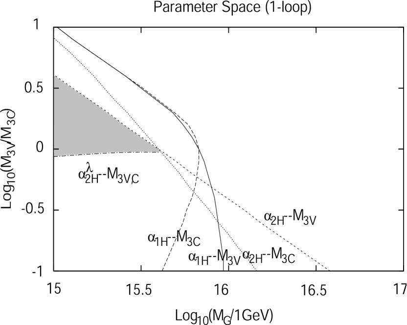
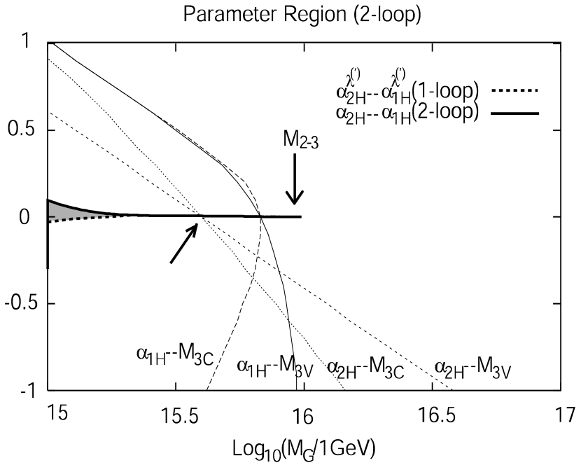
Figure 2: Parameter region of the SU(5)${}_{\rm GUT}\times$U(2)_H model. The parameter space of the model spanned by two free parameters $M_{G}$ and $M_{3V}/M_{3C}$ are restricted by requiring that all the running coupling constants of the model remain finite while the renormalization point is below the heaviest particle of the model. The left panel shows the parameter region, where the 1-loop renormalization group is used for all the coupling constants. The right-hand sides of the four curves labelled “(gauge-coupling)-mass” are excluded. The region below a curve labelled “$\alpha_{\rm 2H}^{\lambda}$–$M_{3V,C}$” is also excluded. Thus, the parameter space of the model is restricted to the shaded triangular region. The right panel shows the parameter region (shaded), where 2-loop effects are included in the renormalization-group equations of gauge coupling constants. The four curves are those found in the left panel; we keep them just because they make it easier to compare the panel with the left one. The majority of the triangular region in the left panel is further excluded because of the 2-loop effects, and only a small region survives near the line $M_{3V}\simeq M_{3C}$. The upper bound of $M_{G}$ is indicated by an arrow. In the right panel, $M_{2-3}$ indicates the unification point between $1/\alpha_{2}$ and $1/\alpha_{3}(+2\sigma)$ (see Fig. 1 for details). It is easy to see that $M_{G}\mathop{}_{\textstyle\sim}^{\textstyle<}10^{15.6}$ GeV $\simeq$ ($10^{-0.4}\simeq 0.40$) $\times$ ($M_{2-3}\simeq 10^{16.0}$ GeV). Both two panels use $\alpha_{s}^{\overline{\rm MS},(5)}(M_{Z})=0.1212$. The effects from the non-renormalizable operator (22) are not included here.

Figure 4: Contour plots of the upper bound of the proton lifetime on the mSUGRA parameter space. The left panel is the prediction of the SU(5)${}_{\rm GUT}\times$U(2)_H model and the right one that of the SU(5)${}_{\rm GUT}\times$U(3)_H model. The upper bound changes as the universal scalar mass $m_{0}$ and the universal gaugino mass $m_{1/2}$ are varied (other mSUGRA parameters are fixed at $\tan\beta=10$, $A_{0}=0.0$). The $\mu$ parameter is chosen to be positive, when the constraint from the branching ratio of the $b\rightarrow s\gamma$ process is less severe. The upper bound of the lifetimes varies as (1.4–3.2)$\times 10^{33}$ yrs in the SU(5)${}_{\rm GUT}\times$U(2)_H model, where the QCD coupling constant $\alpha_{s}^{\overline{\rm MS},(5)}(M_{Z})=0.1212$ is used. The upper bound varies as (1–5)$\times 10^{35}$ yrs in the SU(5)${}_{\rm GUT}\times$U(3)_H model, where the QCD coupling constant $\alpha_{s}^{\overline{\rm MS},(5)}(M_{Z})=0.1132$ is used. In both panels, the effects from non-renormalizable operators are not included. The thick curves labelled $m_{h}$ and $m_{\chi}$ are the bounds on the mSUGRA parameter space from the LEP II experiment in search of the lightest Higgs ($m_{h}\geq 114$ GeV, 95% C.L. ) [40] and the lightest chargino ($m_{\chi}\geq 103.5$ GeV, 95% C.L.) [41]. These curves are obtained by using the SOFTSUSY1.7 code [33]. The excluded region changes when other codes are used; lower bound of $m_{1/2}$ for fixed $m_{0}$ can be higher by about 100 GeV. The code we adopt yields the largest pole mass of the lightest Higgs scalar among various codes available [34], and hence the excluded region is the smallest.

Figure 5: The left panels show the contour plots of the energy scale $M_{2-3}$, where the SU(2)_L and SU(3)_C gauge coupling constants become the same. The right panels show those of the energy scale $M_{1-2}$, where the U(1)_Y and SU(2)_L gauge coupling constants become the same. The upper panels are contour plots on the $(m_{0},m_{1/2})$ parameter space of mSUGRA SUSY breaking, the lower ones are for the $(M_{\rm mess},m_{\rm SUSY}\equiv((1/24)/(4\pi))\Lambda)$ parameter space of the GMSB. Other parameters are fixed for both SUSY breakings; $A_{0}=0$ GeV for mSUGRA SUSY breaking, and $\tan\beta=10.0$ and $\mu>0$ for both SUSY breakings. $\alpha_{s}^{\overline{\rm MS},(5)}(M_{Z})=0.1172$ is used as the QCD coupling constant in this figure. See the caption for Fig. 4 for more details about the region excluded by the LEP II experiments.

References

- [1] E. Witten, Nucl. Phys. B 258 (1985) 75.
-
[2]
N. Sakai and T. Yanagida,
Nucl. Phys. B 197 (1982) 533;
S. Weinberg, Phys. Rev. D 26 (1982) 287. - [3] H. Murayama and A. Pierce, Phys. Rev. D 65 (2002) 055009 [arXiv:hep-ph/0108104]; and references therein.
- [4] Y. Hayato et al. [Super-Kamiokande Collaboration], Phys. Rev. Lett. 83 (1999) 1529 [arXiv:hep-ex/9904020].
- [5] Y. Kawamura, Prog. Theor. Phys. 105 (2001) 999 [arXiv:hep-ph/0012125].
- [6] L. J. Hall and Y. Nomura, Phys. Rev. D 64 (2001) 055003 [arXiv:hep-ph/0103125].
- [7] E. Witten, arXiv:hep-ph/0201018.
- [8] Y. Imamura, T. Watari and T. Yanagida, Phys. Rev. D 64 (2001) 065023 [arXiv:hep-ph/0103251].
- [9] T. Watari and T. Yanagida, Phys. Lett. B 520 (2001) 322 [arXiv:hep-ph/0108057], arXiv:hep-ph/0208107.
- [10] R. Barbieri, G. R. Dvali and A. Strumia, Phys. Lett. B 333 (1994) 79 [arXiv:hep-ph/9404278].
- [11] S. M. Barr, Phys. Rev. D 55 (1997) 6775 [arXiv:hep-ph/9607359].
- [12] M. Dine, Y. Nir and Y. Shadmi, arXiv:hep-ph/0206268.
- [13] I. Izawa and T. Yanagida, Prog. Theor. Phys. 97 (1997) 913 [arXiv:hep-ph/9703350].
- [14] L. J. Hall and Y. Nomura, Phys. Rev. D 66 (2002) 075004 [arXiv:hep-ph/0205067].
- [15] T. Friedmann and E. Witten, arXiv:hep-th/0211269.
- [16] T. Yanagida, Phys. Lett. B 344 (1995) 211 [arXiv:hep-ph/9409329].
- [17] J. Hisano and T. Yanagida, Mod. Phys. Lett. A 10 (1995) 3097 [arXiv:hep-ph/9510277].
- [18] N. Maekawa, Prog. Theor. Phys. 106 (2001) 401 [arXiv:hep-ph/0104200]. N. Maekawa, Phys. Lett. B 521 (2001) 42 [arXiv:hep-ph/0107313].
- [19] Appendix of K. I. Izawa, K. Kurosawa, Y. Nomura and T. Yanagida, Phys. Rev. D 60 (1999) 115016 [arXiv:hep-ph/9904303].
- [20] N. Maekawa and T. Yamashita, Prog. Theor. Phys. 108 (2002) 719 [arXiv:hep-ph/0205185].
- [21] M. Fujii and T. Watari, Phys. Lett. B 527 (2002) 106 [arXiv:hep-ph/0112152].
- [22] T. Watari, Ph.D thesis.
- [23] J. Hisano, H. Murayama and T. Yanagida, Nucl. Phys. B 402 (1993) 46 [arXiv:hep-ph/9207279].
- [24] G. F. Giudice and A. Masiero, Phys. Lett. B 206 (1988) 480.
- [25] I. Antoniadis, C. Kounnas and K. Tamvakis, Phys. Lett. B 119 (1982) 377.
- [26] M. T. Grisaru and W. Siegel, Nucl. Phys. B 201 (1982) 292 [Erratum, ibid. B 206 (1982) 496]; P. S. Howe, K. S. Stelle and P. C. West, Phys. Lett. B 124 (1983) 55.
- [27] N. Arkani-Hamed and H. Murayama, JHEP 0006 (2000) 030 [arXiv:hep-th/9707133].
- [28] R. Barbieri, S. Ferrara, L. Maiani, F. Palumbo and C. A. Savoy, Phys. Lett. B 115 (1982) 212; B. de Wit, P. G. Lauwers and A. Van Proeyen, Nucl. Phys. B 255 (1985) 569; P. C. Argyres, M. Ronen Plesser and N. Seiberg, Nucl. Phys. B 471 (1996) 159 [arXiv:hep-th/9603042].
- [29] K. Hagiwara et al. [Particle Data Group Collaboration], Phys. Rev. D 66 (2002) 010001.
- [30] S. Aoki et al. [JLQCD Collaboration], Phys. Rev. D 62 (2000) 014506 [arXiv:hep-lat/9911026].
- [31] J. Hisano, arXiv:hep-ph/0004266.
- [32] L. E. Ibañez and C. Muñoz, Nucl. Phys. B 245 (1984) 425.
- [33] B. C. Allanach, Comput. Phys. Commun. 143 (2002) 305 [arXiv:hep-ph/0104145].
- [34] B. C. Allanach, S. Kraml and W. Porod, arXiv:hep-ph/0302102.
- [35] S. Raby, arXiv:hep-ph/0211024.
- [36] Y. Suzuki et al. [TITAND Working Group Collaboration], arXiv:hep-ex/0110005.
- [37] M. Shiozawa et al. [Super-Kamiokande Collaboration], Phys. Rev. Lett. 81 (1998) 3319 [arXiv:hep-ex/9806014].
- [38] N. Arkani-Hamed, H. C. Cheng and T. Moroi, Phys. Lett. B 387 (1996) 529 [arXiv:hep-ph/9607463].
- [39] K. Kurosawa, N. Maru and T. Yanagida, Phys. Lett. B 512 (2001) 203 [arXiv:hep-ph/0105136].
- [40] LEP Higgs Working Group Collaboration, arXiv:hep-ex/0107030.
-
[41]
LEP II Supersymmetry Working Group,
http://lepsusy.web.cern.ch/lepsusy/www/inos_moriond01/charginos_pub.html. - [42] C. M. Hull, A. Karlhede, U. Lindstrom and M. Rocek, Nucl. Phys. B 266 (1986) 1.
- [43] C. Bachas, C. Fabre and T. Yanagida, Phys. Lett. B 370 (1996) 49 [arXiv:hep-th/9510094].