QCD potential as a “Coulomb–plus–linear” potential

We show analytically that the QCD potential can be expressed, up to an ${\cal O}(\Lambda_{\rm QCD}^{3}r^{2})$ uncertainty, as the sum of a “Coulomb” potential (with log corrections at short distances) and a linear potential, within an approximation based on perturbative expansion in $\alpha_{S}$ and the renormalon dominance picture. The expansion of $V_{\rm QCD}(r)$ is truncated at ${\cal O}(\alpha_{S}^{N})$ [$N\!=\!6\pi/(\beta_{0}\alpha_{S})$], where the term becomes minimal according to the estimate by NLO renormalon, and is studied for $N\gg 1$. Analytic expressions for the linear potential are obtained in some cases.

1 Introduction

Analyses of the static QCD potential $V_{\rm QCD}(r)$ within perturbative QCD entered a new phase when the cancellation of the leading order (LO) renormalons between the QCD potential and the pole masses of quark and antiquark was discovered [1]. Convergence of the perturbative series improved dramatically and much more accurate perturbative predictions became available. Subsequently, several studies [2, 3, 4, 5, 6] showed that perturbative predictions for $V_{\rm QCD}(r)$ agree well with phonomenological potentials (determined from heavy quarkonium spectroscopy) and lattice calculations of $V_{\rm QCD}(r)$, once the LO renormalon contained in the QCD potential is cancelled (see also [7]). In fact the agreement holds within the perturbative uncertainty of ${\cal O}(\Lambda_{\rm QCD}^{3}r^{2})$ estimated from the residual next-to-leading order (NLO) renormalon [8]. Despite of different prescriptions used for cancelling the LO renormalon, all these perturbative predictions were mutually consistent within the ${\cal O}(\Lambda_{\rm QCD}^{3}r^{2})$ uncertainty. These observations indicate validity of the renormalon dominance picture for the QCD potential.

Empirically it is known that phenomenological potentials and lattice computations of $V_{\rm QCD}(r)$ are both approximated well by the sum of a Coulomb potential and a linear potential in the range $r\hbox{ \raise 3.0pt\hbox to0.0pt{$>$}\raise-3.0pt\hbox{$\sim$} }0.5~{}{\rm GeV}^{-1}$ [9]. The linear behavior at large distances is consistent with the quark confinement picture. For this reason, before the discovery of the renormalon cancellation, it was often said that perturbative QCD is unable to explain the “Coulomb-plus-linear” behavior of the QCD potential.

Once the cancellation of the LO renormalons is incorporated, the perturbative QCD potential gets steeper than the Coulomb potential at large distances. This feature can be understood, within perturbative QCD, as an effect of the running of the strong coupling constant [10, 2, 3]. On the other hand, it is not obvious whether the QCD potential is rendered to a “Coulomb-plus-linear” form by this effect. The perturbative uncertainty due to the residual renormalon is of ${\cal O}(r^{2})$, hence there is a possibility that the ${\cal O}(r)$ term of the potential at $r\hbox{ \raise 3.0pt\hbox to0.0pt{$<$}\raise-3.0pt\hbox{$\sim$} }\Lambda_{\rm QCD}^{-1}$ is predictable within perturbative QCD. In this paper, by considering a certain limit of a finite-order perturbative expansion of $V_{\rm QCD}(r)$ based on the renormalon dominance picture, we show that indeed the potential can be decomposed into a “Coulomb-plus-linear” form, up to an ${\cal O}(\Lambda_{\rm QCD}^{3}r^{2})$ uncertainty. Our prescription gives a prediction consistent with the previous predictions [2, 3, 4, 5, 6].

In Sec. 2 we set up our conventions for our analysis. Sec. 3 presents an analysis in the large–$\beta_{0}$ approximation; Sec. 4 presents an analysis based on renormalization-group (RG), incorporating 1-, 2-, and 3-loop running of the coupling constant. Discussion and conclusions are given in Secs. 5 and 6, respectively.

2 Perturbative QCD potential and renormalons

The static QCD potential is defined from an expectation value of the Wilson loop as

$$V_{\rm QCD}(r) = -\lim_{T\to\infty}\frac{1}{iT}\,\ln\frac{\left<{0}\,\right|{\rm{Tr\,P}}\exp\biggl{[}ig_{S}\oint_{\cal P}dx^{\mu}\,A_{\mu}(x)\biggr{]}\left|\,{0}\,\right>}{\left<{0}\,\right|{\rm Tr}\,{\bf 1}\left|\,{0}\,\right>}$$ (1)

$$= \int\frac{d^{3}\vec{q}}{(2\pi)^{3}}\,e^{i\vec{q}\cdot\vec{r}}\,\biggl{[}-4\pi C_{F}\,\frac{\alpha_{V}(q)}{q^{2}}\biggr{]}~{}~{}~{};~{}~{}~{}~{}~{}q=|\vec{q}|,$$

where ${\cal P}$ is a rectangular loop of spatial extent $r$ and time extent $T$. The second line defines the $V$-scheme coupling contant, $\alpha_{V}(q)$, in momentum space; $C_{F}=4/3$ is the second Casimir operator of the fundamental representation. In perturbative QCD, $\alpha_{V}(q)$ is calculable in a series expansion of the strong coupling constant:

$$\alpha_{V}(q)=\alpha_{S}\,\sum_{n=0}^{\infty}P_{n}(\ln(\mu/q))\,\biggl{(}\frac{\alpha_{S}}{4\pi}\biggr{)}^{n}=\alpha_{S}(q)\,\sum_{n=0}^{\infty}a_{n}\,\biggl{(}\frac{\alpha_{S}(q)}{4\pi}\biggr{)}^{n}~{}~{}~{};~{}~{}~{}a_{n}=P_{n}(0).$$ (2)

Here, $P_{n}(\ell)$ denotes an $n$-th-degree polynomial of $\ell$. In this paper, unless the argument is specified explicitly, $\alpha_{S}\equiv\alpha_{S}(\mu)$ denotes the strong coupling constant renormalized at the renormalization scale $\mu$, defined in the $\overline{\rm MS}$ scheme. The series expansion of $\alpha_{S}(q)$ in terms of $\alpha_{S}$ is determined by the RG equation

$$q^{2}\,\frac{d}{dq^{2}}\,\alpha_{S}(q)=-\alpha_{S}(q)\sum_{n=0}^{\infty}\beta_{n}\biggl{(}\frac{\alpha_{S}(q)}{4\pi}\biggr{)}^{n+1},$$ (3)

where $\beta_{n}$ represents the $(n+1)$-loop coefficient of the beta function. Therefore, at each order of the expansion of $\alpha_{V}(q)$ in $\alpha_{S}$, the only part of the polynomial $P_{n}(\ln(\mu/q))$ that is not determined by the RG equation is $a_{n}$. The above equations fix our conventions.

It is known [11] that $a_{n}$ for $n\geq 3$ contain infrared (IR) divergences. We will discuss this issue in Sec. 5, whereas in Secs. 3 and 4 we treat $a_{n}$ as finite constants.

According to the renormalon dominance picture, the leading behavior of the ${\cal O}(\alpha_{S}^{n+1})$ term of $V_{\rm QCD}(r)$ at large orders is given by the LO renormalon contribution as $V^{(n)}_{\rm QCD}(r)\sim{const.}\times n!\,(\beta_{0}\alpha_{S}/(2\pi))^{n}\,n^{\delta/2}$, where $\delta=\beta_{1}/\beta_{0}^{2}$ [12]. In the computation of the heavy quarkonium spectrum, the LO renormalon gets cancelled against the LO renormalons contained in the quark and antiquark pole masses. Considering this application, if we subtract the LO renormalon contribution from $V^{(n)}_{\rm QCD}(r)$, its large-order behavior becomes ${const}.\times r^{2}\,n!\,(\beta_{0}\alpha_{S}/(6\pi))^{n}\,n^{3\delta/2}$ due to the NLO renormalon contribution. Then $V^{(n)}_{\rm QCD}(r)$ (after the LO renormalon is subtracted) becomes minimal at $n\approx N\equiv 6\pi/(\beta_{0}\alpha_{S})$ and its size scarcely changes for $N-\sqrt{N}\ll n\ll N+\sqrt{N}$.

In view of the usual property of asymptotic series, we simply truncate the series expansion of the potential at the order where the term becomes minimal according to the renormalon dominance picture, i.e. at ${\cal O}(\alpha_{S}^{N})$:

$$V_{N}(r)\equiv[V_{\rm QCD}(r)]_{N}=-4\pi C_{F}\,\int\frac{d^{3}\vec{q}}{(2\pi)^{3}}\,\frac{e^{i\vec{q}\cdot\vec{r}}}{q^{2}}\,[{\alpha_{V}(q)}]_{N}.$$ (4)

Here and hereafter, $[X]_{N}$ denotes the series expansion of $X$ in $\alpha_{S}$ truncated at ${\cal O}(\alpha_{S}^{N})$. The purpose of this paper is to examine $V_{N}(r)$ for $N\gg 1$ while keeping $\Lambda_{\overline{\rm MS}}$ [13] finite, using certain estimates for the all order terms in Eq. (2). The motivation for considering the large $N$ limit is that it corresponds to the limits where the perturbative expansion becomes well-behaved (small expansion parameter) and where the estimate of $V^{(n)}_{\rm QCD}(r)$ by renormalon contribution becomes a better approximation around $n\sim N$. Note that large $N$ corresponds to small $\alpha_{S}$ and large $\mu$ due to the relation between $N$ and $\alpha_{S}$.

Clearly, $V_{N}(r)$ cannot be written as a “Coulomb-plus-linear” form for finite $N$, since it is given as the Coulomb potential ($-C_{F}\alpha_{S}/r$) times an $(N\!-\!1)$-th-degree polynomial of $\ln(\mu r)$, and therefore, $V_{N}(r)\to 0$ as $r\to\infty$. We will see, however, that $V_{N}(r)$ tends to a “Coulomb-plus-linear” potential (plus a quadratic potential) in the large $N$ limit.

3 $V_{N}(r)$ in large–$\beta_{0}$ approximation

The large–$\beta_{0}$ approximation [14] is an empirically successful method for estimating higher-order corrections in perturbative QCD calculations. For $V_{\rm QCD}(r)$, this approximation corresponds to setting $a_{n}=(5\beta_{0}/3)^{n}$ and all $\beta_{n}=0$ except $\beta_{0}$. (Therefore, it includes only the one-loop running of $\alpha_{S}(q)$.) In this section, with these estimates of the all-order terms of $V_{\rm QCD}(r)$, we examine $V_{N}(r)$ for $N\gg 1$. The reasons for examining the large–$\beta_{0}$ approximation are as follows. First, because this approximation leads to the renormalon dominance picture; in fact, the renormalon dominance picture has often been discussed in this approximation. Secondly, as stated in Sec. 1, the running of the strong coupling constant makes the potential steeper at large distances as compared to the Coulomb potential; hence, we would like to see if the potential can be written as a “Coulomb-plus-linear” potential when only the one-loop running is incorporated as a simplest case. We first present the results, discuss some properties, and then sketch how we derived our results.
Results

We define $\widetilde{\Lambda}=e^{5/6}\,\Lambda_{\overline{\rm MS}}^{\mbox{\scriptsize 1-loop}}$, where $\Lambda_{\overline{\rm MS}}^{\mbox{\scriptsize 1-loop}}=\mu\exp[-2\pi/(\beta_{0}\alpha_{S})]$. In this section, we assume $e^{-5/6}\,\mu^{-1}=\widetilde{\Lambda}^{-1}e^{-N/3}\ll r\ll\widetilde{\Lambda}^{-1}e^{N/3}$ when taking various limits. Note that, as $N\to\infty$, the lower bound ($e^{-5/6}\,\mu^{-1}$) and the upper bound ($\widetilde{\Lambda}^{-1}e^{N/3}$) of $r$ go to 0 and $\infty$, respectively.

$V_{N}(r)$ for $N\gg 1$ within the large–$\beta_{0}$ approximation can be decomposed into four parts corresponding to {$r^{-1}$, $r^{0}$, $r^{1}$, $r^{2}$} terms (with logarithmic corrections in the $r^{-1}$ and $r^{2}$ terms):

$$V_{N}^{(\beta_{0})}(r)=\frac{4C_{F}}{\beta_{0}}\,\widetilde{\Lambda}\,\,v(\widetilde{\Lambda}r,N),$$ (5)

$$v(\rho,N)=v_{C}(\rho)+B(N)+C\rho+D(\rho,N)+(\mbox{terms that vanish as $N\to\infty$}).$$ (6)

(i)“Coulomb” part:

$$v_{C}(\rho)=-\frac{\pi}{\rho}+\frac{1}{\rho}\int_{0}^{\infty}dx\,e^{-x}\,\arctan\biggl{[}\frac{\pi/2}{\ln(\rho/x)}\biggr{]},$$ (7)

where $\arctan x\in[0,\pi)$. The asymptotic forms are given by

$$\left\{\begin{array}[]{ll}v_{C}(\rho)\sim-\,\frac{\pi}{2\rho\ln(1/\rho)},{}{}{}&\rho\to 0\\ v_{C}(\rho)\sim-\,\frac{\pi}{\rho},&\rho\to\infty\\ \end{array}\right.$$ (10)

and both asymptotic forms are smoothly interpolated in the intermediate region.

(ii) constant part:

$$B(N)=-\int_{0}^{\infty}dt\,\frac{e^{-t}}{t}\,\biggl{[}\Bigl{(}1+\frac{3}{N}\,t\,\Bigr{)}^{N}-1\biggr{]}-\ln 2-\frac{9}{8N}+\frac{99}{64N^{2}}.$$ (11)

The first term (integral) diverges rapidly for $N\to\infty$ as ${\displaystyle-\,\frac{3}{2}\sqrt{\frac{2\pi}{N}}\biggl{(}\frac{3}{e^{2/3}}\biggr{)}^{N}\,\bigl{[}\,1+{\cal O}(1/N)\bigr{]}}$.

(iii) linear part:

$$C=\frac{\pi}{2}.$$ (12)

(iv) quadratic part:

$$D(\rho,N)=\rho^{2}\,\biggl{[}\frac{1}{12}\ln N+d(\rho)\biggr{]},$$ (13)

$$d(\rho)=-\int_{0}^{\infty}dx\,\,\frac{e^{-x}-\Bigl{[}1-x+\frac{1}{2}x^{2}-\frac{1}{6}x^{3}\,\theta(1-x)\Bigr{]}}{x^{4}}\,\,\frac{\ln(\rho/x)}{\ln^{2}(\rho/x)+\pi^{2}/4}$$

$$~{}~{}~{}~{}~{}~{}~{}~{}-\frac{1}{12}\,\biggl{[}\ln\Bigl{(}\ln^{2}\!\rho+\frac{\pi^{2}}{4}\Bigr{)}+\ln\frac{9}{2}+\gamma_{E}\biggr{]},$$ (14)

where $\theta(x)$ is the unit step function and $\gamma_{E}=0.5772...$ is the Euler constant. The asymptotic forms of $d(\rho)$ are given by

$$\left\{\begin{array}[]{ll}\rule[-11.38109pt]{0.0pt}{17.07164pt}d(\rho)\sim-\frac{1}{12}\,\Bigl{[}2\ln\ln\frac{1}{\rho}+\ln\frac{9}{2}+\gamma_{E}\Bigr{]},{}{}{}&\rho\to 0\\ d(\rho)\sim-\frac{1}{12}\,\Bigl{[}2\ln\ln{\rho}+\ln\frac{9}{2}+\gamma_{E}\Bigr{]},&\rho\to\infty\\ \end{array}\right.$$ (17)

and in the intermediate region both asymptotic forms are smoothly interpolated.

Although the constant part of $V_{N}^{(\beta_{0})}(r)$ diverges rapidly as $N\to\infty$, the divergence can be absorbed into the quark masses in the computation of the heavy quarkonium spectrum. Therefore, in our analysis, we will not be concerned with the constant part of the potential but only with the $r$-dependent terms.

The quadratic part of $V_{N}^{(\beta_{0})}(r)$ diverges slowly as $\widetilde{\Lambda}^{3}r^{2}\ln N\sim\widetilde{\Lambda}^{3}r^{2}\ln\ln(\mu/\widetilde{\Lambda})$. We may consider this feature to be a characteristic property of renormalons for the following reasons. (1) If the series expansion of $m_{\rm pole}(m_{\overline{\rm MS}},\alpha_{S})$ or $V_{\rm QCD}(r)$ is truncated at the order corresponding to the minimal term of the LO renormalon contribution, i.e. $N^{\prime}=2\pi/(\beta_{0}\alpha_{S})$, $[m_{\rm pole}]_{N^{\prime}}$ or $[V_{\rm QCD}(r)]_{N^{\prime}}$ diverges as $\widetilde{\Lambda}\ln N^{\prime}$ (within the large-$\beta_{0}$ approximation). We may compare $\widetilde{\Lambda}\ln N^{\prime}$ with the usual interpretation that $m_{\rm pole}$ and $V_{\rm QCD}(r)$ contain ${\cal O}(\widetilde{\Lambda})$ perturbative uncertainties due to the LO renormalons. (2) We have checked that even if we incorporate the effect of the two-loop running, i.e. even if we set $\beta_{1}\neq 0$, the quadratic part of $V_{N}(r)$ still diverges as $\widetilde{\Lambda}^{3}r^{2}\ln N$. Therefore, we interpret that the quadratic part of $V_{N}^{(\beta_{0})}(r)$ represents an ${\cal O}(\widetilde{\Lambda}^{3}r^{2})$ uncertainty, following the standard interpretation on the perturbative uncertainty induced by the NLO renormalon.

\psfrag{rho=Lambda*r}{\hskip 28.45274pt$\rho=\widetilde{\Lambda}\,r$}\psfrag{vc(rho)+C*rho}{$v_{C}(\rho)+C\rho$}\psfrag{lefttitle}{\hskip 2.84526pt$v(\rho,N)\!-\!B(N)$ and $v_{C}(\rho)\!+\!C\rho$}\psfrag{N=10}{$N=10$}\psfrag{N=30}{$\!\!N=30$}\psfrag{N=100}{$\!\!N=100$}\psfrag{r=1/Lambda}{$r=1/\widetilde{\Lambda}$}\psfrag{r=1/LambdaMS}{$r=1/\Lambda_{\overline{\rm MS}}^{\mbox{\scriptsize 1-loop}}$}\includegraphics[width=284.52756pt]{VN-CplusL.eps}

Figure 1: Truncated potential after the constant term is subtracted, $v(\rho,N)-B(N)$, (dashed black) vs. $\rho$ for $N=10$, 30, 100. “Coulomb-plus-linear” potential, $v_{C}(\rho)+C\rho$, (solid red) is also plotted, which is hardly distinguishable from the $N=30$ curve.

In this respect, we note that the dependence of $V_{N}^{(\beta_{0})}(r)$ on $N$ is mild; for instance, as shown in Fig. 1, the variation of $V_{N}^{(\beta_{0})}(r)$ is small (after the constant part is subtracted) in the range $r\hbox{ \raise 3.0pt\hbox to0.0pt{$<$}\raise-3.0pt\hbox{$\sim$} }\widetilde{\Lambda}^{-1}$ as we vary $N$ from 10 to 100; it corresponds to a variation of $\mu/\Lambda_{\overline{\rm MS}}^{\mbox{\scriptsize 1-loop}}$ from 30 to $3\times 10^{14}$.

The “Coulomb” part and the linear part are finite as $N\to\infty$. In Fig. 1, we see that $V_{N}^{(\beta_{0})}(r)$ is approximated fairly well by the sum of the “Coulomb” part and the linear part (up to an $r$-independent constant) in the region $r\hbox{ \raise 3.0pt\hbox to0.0pt{$<$}\raise-3.0pt\hbox{$\sim$} }\widetilde{\Lambda}^{-1}$ when we vary $N$ between 10 and 100. Moreover, as long as $\frac{1}{12}\ln N\hbox{ \raise 3.0pt\hbox to0.0pt{$<$}\raise-3.0pt\hbox{$\sim$} }{\cal O}(1)$, the difference between $V_{N}^{(\beta_{0})}(r)$ and the “Coulomb-plus-linear” potential remains at or below ${\cal O}(\widetilde{\Lambda}^{3}r^{2})$ in the entire range of $r$.
Outline of derivation

Let us write $L=\frac{\beta_{0}\alpha_{S}}{2\pi}\ln\Bigl{(}\frac{\mu e^{5/6}}{q}\Bigr{)}=1+\frac{3}{N}\ln\Bigl{(}\frac{\widetilde{\Lambda}}{q}\Bigr{)}$. $V_{N}^{(\beta_{0})}(r)$ is defined as the Fourier transform of $(4\pi C_{F}\alpha_{S}/q^{2})\sum_{n=0}^{N-1}L^{n}=(4\pi C_{F}\alpha_{S}/q^{2})(1-L^{N})/(1-L)$. After integration over angular variables, it is given by

$$V_{N}^{(\beta_{0})}(r)=-\frac{2C_{F}\alpha_{S}}{\pi}\int_{0}^{\infty}dq\,\frac{\sin(qr)}{qr}\,\frac{1-L^{N}}{1-L}=\frac{4C_{F}}{\beta_{0}}\Bigl{[}v_{1}(\widetilde{\Lambda}r)+v_{2}(\widetilde{\Lambda}r,N)\Bigr{]},$$ (18)

where we separated the integral into two parts after deforming the integral contour slightly:

$$v_{1}(\rho)={\rm Im}\int_{0}^{\infty}\!dk\,\frac{e^{ik\rho}}{k\rho}\,\frac{1}{\ln(1/k)-i\epsilon}=-\frac{1}{\rho}\,{\rm Im}\int_{0}^{\infty}\!dx\,e^{-x}\,\ln\biggl{[}\ln\Bigl{(}\frac{\rho}{x}\Bigr{)}-\frac{i\pi}{2}\biggr{]},~{}~{}~{}$$ (19)

$$v_{2}(\rho,N)=-{\rm Im}\int_{0}^{\infty}dk\,\frac{e^{ik\rho}}{k\rho}\,\frac{1}{\ln(1/k)-i\epsilon}\biggl{[}1+\frac{3}{N}\ln\Bigl{(}\frac{1}{k}\Bigr{)}\biggr{]}^{N}$$

$$~{}~{}~{}~{}~{}~{}~{}~{}~{}~{}~{}=-\frac{\pi\cos\rho}{\rho}-{\rm Pr.}\int_{0}^{\infty}\!dk\,\frac{\sin(k\rho)}{k\rho}\,\frac{1}{\ln(1/k)}\biggl{[}1+\frac{3}{N}\ln\Bigl{(}\frac{1}{k}\Bigr{)}\biggr{]}^{N}.$$ (20)

$v_{1}$ and $v_{2}$ are defined by the first equalities of (19) and (20), respectively. Contributions from the pole at $k=1$ in $v_{1}$ and $v_{2}$ cancel, since the original integral (18) does not contain a pole at $q=\widetilde{\Lambda}$. In the second equality of (19), we deformed the integral contour into the upper half plane on the complex $k$-plane and integrated by parts. As for $v_{2}$, since $[1+\frac{3}{N}\ln\Bigl{(}\frac{1}{k}\Bigr{)}]^{N}\to 1/k^{3}$ as $N\to\infty$, the constant ($\rho^{0}$) and quadratic ($\rho^{2}$) terms in the integral become IR divergent in this limit. On the other hand, the negative power of $k$ induces the positive power behavior of $\rho$, i.e. the linear and quadratic terms, in $v_{2}$ in the large $N$ limit. We define

$$v_{2}(\rho,N)=\frac{A}{\rho}+B(N)+C\rho+D(\rho,N)+(\mbox{terms that vanish as $N\to\infty$}),$$ (21)

where $D(\rho,N)={\cal O}(\rho^{2})$. In computing $A$ and $C$, it is convenient to first remove divergences by subtracting appropriate constant and quadratic terms from $v_{2}$. Let

$$\tilde{v}_{2}(\rho,N,k_{0})\equiv-\frac{\pi\cos\rho}{\rho}-{\rm Pr.}\int_{0}^{\infty}\!dk\,\biggl{[}\frac{\sin(k\rho)}{k\rho}-\theta(k_{0}-k)\biggl{\{}1-\frac{1}{6}(k\rho)^{2}\biggr{\}}\biggr{]}$$

$$~{}~{}~{}~{}~{}~{}~{}~{}~{}~{}~{}~{}~{}~{}~{}~{}~{}~{}~{}~{}~{}~{}~{}~{}~{}~{}~{}~{}~{}~{}~{}~{}~{}~{}~{}~{}~{}~{}~{}~{}~{}~{}~{}~{}~{}~{}~{}~{}~{}~{}~{}~{}~{}~{}~{}~{}~{}~{}~{}~{}~{}~{}~{}\times\,\frac{1}{\ln(1/k)}\biggl{[}1+\frac{3}{N}\ln\Bigl{(}\frac{1}{k}\Bigr{)}\biggr{]}^{N},$$ (22)

where $k_{0}=2$ is an IR cutoff. Now we may send $N\to\infty$ before integration over $k$. $\tilde{v}_{2}(\rho,\infty,k_{0})$ is finite for $0<\rho<\infty$ and differs from ${v}_{2}(\rho,N)$ only by constant ($\rho^{0}$) and quadratic ($\rho^{2}$) terms, apart from terms that vanish as $N\to\infty$. One can show that the $\rho^{-1}$ and $\rho^{1}$ terms stem only from the first term of (22):

$$A=\lim_{\rho\to 0}\,\rho\,\tilde{v}_{2}(\rho,\infty,k_{0})=-\pi,$$ (23)

$$C=\lim_{\rho\to 0}\frac{1}{2}\frac{\partial^{2}}{\partial\rho^{2}}[\rho\,\tilde{v}_{2}(\rho,\infty,k_{0})]=\frac{\pi}{2}.$$ (24)

The constant and quadratic terms can be calculated directly from $v_{2}$:

$$B(N)=\lim_{\rho\to 0}\frac{\partial}{\partial\rho}[\rho\,v_{2}(\rho,N)]$$

$$~{}~{}~{}~{}~{}~{}~{}~{}=-\int_{\epsilon}^{\infty}dt\,\frac{e^{-t}}{t}\,\Bigl{(}1+\frac{3}{N}\,t\,\Bigr{)}^{N}-\int_{-\infty}^{-\epsilon}dt\,\frac{e^{2t}}{t}\,\Bigl{(}1-\frac{9}{2N}\,t^{2}+\cdots\,\Bigr{)},$$ (25)

$$D(\rho,N)=v_{2}(\rho,N)-\biggl{[}\frac{A}{\rho}+B(N)+C\rho\biggr{]}.$$ (26)

In the second equality of (25) we set $t=\ln(1/k)$ and expanded the integrand in $1/N$ in the region $t<0$. It is then straightforward to obtain (11). One may separate a divergent part as $N\to\infty$ from (26) in a similar manner. As for the finite part ($N$-independent part), we deform the integral contour into the upper half $k$-plane to obtain (13),(14). Finally $v_{C}(\rho)$ is given by the sum of $A/\rho$ and $v_{1}(\rho)$. The asymptotic forms of $v_{C}(\rho)$ and $d(\rho)$ are obtained by expanding the integrands in $\ln x$.

We made a cross check of our results by comparing $v(\rho,N)$ and $v_{C}(\rho)+B(N)+C\rho+D(\rho,N)$ numerically for $3\leq N\leq 1000$, after subtracting the divergent terms from both. The difference diminishes swiftly with $N$.

4 $V_{N}(r)$ with 1-, 2-, and 3-loop running of $\alpha_{S}(q)$

In this section we examine $V_{N}(r)$ in three cases corresponding to the following estimates of the all order terms of $V_{\rm QCD}(r)$:
(a) [1-loop running] $\beta_{0}$, $a_{0}$: exact values, $\beta_{n}=a_{n}=0$ ($n\geq 1$);
(b) [2-loop running] $\beta_{0}$, $\beta_{1}$, $a_{0}$, $a_{1}$: exact values, $\beta_{n}=a_{n}=0$ ($n\geq 2$);
(c) [3-loop running] $\beta_{0}$, $\beta_{1}$, $\beta_{2}$, $a_{0}$, $a_{1}$, $a_{2}$: exact values [16, 17], $\beta_{n}=a_{n}=0$ ($n\geq 3$).
We assume $\beta_{0},\,\beta_{1},\,\beta_{2},a_{0},a_{1},a_{2}\,({\rm exact})>0$. In the standard 1-, 2-, and 3-loop RG improvements of $V_{\rm QCD}(r)$, the same all-order terms as in the above cases are resummed; the difference of our treatment is that the perturbative expansions are truncated at ${\cal O}(\alpha_{S}^{N})$. We note that the renormalon dominance picture is consistent with the above estimates of higher-order terms, or more generally, with the RG analysis [12]. All the results for the case (a) can be obtained if we replace $\widetilde{\Lambda}$ by $\Lambda_{\overline{\rm MS}}^{\mbox{\scriptsize 1-loop}}$ in the results of the large–$\beta_{0}$ approximation in Sec. 3.

Similarly to the previous section, we can decompose $V_{N}(r)$ into four parts:

$$V_{N}(r)=V_{C}(r)+{\cal B}(N)+{\cal C}\,r+{\cal D}(r,N)+(\mbox{terms that vanish as $N\to\infty$}),$$ (27)

where

$$V_{C}(r)=-\frac{4\pi C_{F}}{\beta_{0}r}-\frac{2C_{F}}{\pi}\,{\rm Im}\int_{C_{1}}\!dq\,\frac{e^{iqr}}{qr}\,\alpha_{V}(q),$$ (28)

$${\cal B}(N)=\lim_{r\to 0}\,\frac{2C_{F}}{\pi}\,{\rm Re}\int_{C_{1}}\!dq\,e^{iqr}\,\Bigl{\{}\alpha_{V}(q)-[\alpha_{V}(q)]_{N}\Bigr{\}},$$ (29)

$${\cal C}=\frac{C_{F}}{2\pi i}\int_{C_{2}}\!dq\,q\,\alpha_{V}(q),$$ (30)

$${\cal D}(r,N)=V_{N}(r)-[V_{C}(r)+{\cal B}(N)+{\cal C}\,r].$$ (31)

\psfrag{C1}{$C_{1}$}\psfrag{q}{$q$}\psfrag{q*}{$q_{*}$}\psfrag{0}{\raise-2.84526pt\hbox{$0$}}\includegraphics[width=128.0374pt]{path1.eps}	\psfrag{C2}{$C_{2}$}\psfrag{q}{$q$}\psfrag{q*}{$q_{*}$}\psfrag{0}{\raise-2.84526pt\hbox{$0$}}\includegraphics[width=128.0374pt]{path2.eps}
(i)	(ii)

Figure 2: Integral contours $C_{1}$ and $C_{2}$ on the complex $q$-plane. $q_{*}$ denotes the Landau singularity of $\alpha_{S}(q)$. For 1-loop running, $q_{*}$ is a pole; for 2- and 3-loop running, $q_{*}$ is a branch point. In the latter case, branch cut is on the real axis starting from $q_{*}$ to $-\infty$.

The integral contours $C_{1}$ and $C_{2}$ are displayed in Figs. 2(i),(ii), respectively.

The coefficient of the linear potential can be expressed analytically for (a),(b),(c). In the first two cases, the expressions read

$${\cal C}^{(a)}=\frac{2\pi C_{F}}{\beta_{0}}\,\Bigl{(}\Lambda_{\overline{\rm MS}}^{\mbox{\scriptsize 1-loop}}\Bigr{)}^{2},$$ (32)

$${\cal C}^{(b)}=\frac{2\pi C_{F}}{\beta_{0}}\,\Bigl{(}\Lambda_{\overline{\rm MS}}^{\mbox{\scriptsize 2-loop}}\Bigr{)}^{2}\,\frac{e^{-\delta}}{\Gamma(1+\delta)}\,\biggl{[}1+\frac{a_{1}}{\beta_{0}}\,\delta^{-1-\delta}\,e^{\delta}\,\gamma(1+\delta,\delta)\biggr{]},$$ (33)

where $\gamma(x,\tau)\equiv\int_{0}^{\tau}dt\,t^{x-1}\,e^{-t}$ represents the incomplete gamma function; $\Lambda_{\overline{\rm MS}}^{\mbox{\scriptsize 1-loop}}$ and $\Lambda_{\overline{\rm MS}}^{\mbox{\scriptsize 2-loop}}$ denote the Lambda parameters in the $\overline{\rm MS}$ scheme; $\delta=\beta_{1}/\beta_{0}^{2}$. In the case (c), ${\cal C}$ can be expressed in terms of confluent hypergeometric functions except for the coefficient of $a_{2}$, while the coefficient of $a_{2}$ can be expressed in terms of generalized confluent hypergeometic functions. Since, however, the expression is lengthy and not very illuminating, we do not present it here.

The asymptotic behaviors of $V_{C}(r)$ for $r\to 0$ are same as those of $V_{\rm QCD}(r)$ in the respective cases, as determined by RG equations. The asymptotic behaviors of $V_{C}(r)$ for $r\to\infty$ are given by $-4\pi C_{F}/(\beta_{0}r)$ [the first term of eq. (28)] in all the cases.

As for ${\cal B}(N)$ and ${\cal D}(r,N)$, we have not obtained simple expressions in the cases (b),(c), since analytic treatments are more difficult than in the case (a): we have not separated the divergent parts as $N\to\infty$ nor obtained the asymptotic forms for $r\to 0$, $r\to\infty$. Based on some analytic examinations, together with numerical examinations for $N\leq 30$, we conjecture that ${\cal B}(N)$ and ${\cal D}(r,N)$ in the cases (b),(c) have behaviors similar to those in the case (a).

Let us compare the “Coulomb–plus–linear” potential, $V_{C}(r)+{\cal C}\,r$, for the three cases when the number of quark flavors is zero. We also compare them with lattice calculations of the QCD potential in the quenched approximation. See Fig. 3. We take the input parameter for $V_{C}(r)+{\cal C}\,r$ as $\alpha_{S}(Q)=0.2$, which corresponds to $\Lambda_{\overline{\rm MS}}^{\mbox{\scriptsize 1-loop}}/Q=0.057$, $\Lambda_{\overline{\rm MS}}^{\mbox{\scriptsize 2-loop}}/Q=0.13$, $\Lambda_{\overline{\rm MS}}^{\mbox{\scriptsize 3-loop}}/Q=0.12$. Then, the scale for each lattice data set is fixed using the central value of the relation [18] $\Lambda_{\overline{\rm MS}}^{\mbox{\scriptsize 3-loop}}\,r_{0}=0.602(48)$, where $r_{0}$ is the Sommer scale. An arbitrary $r$-independent constant has been added to each potential and each lattice data set to facilitate the comparison.

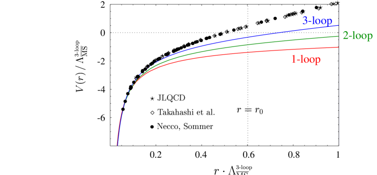
Figure 3: Comparison of $V_{C}(r)+{\cal C}\,r$ corresponding to the cases (a),(b),(c) (solid lines) and the lattice data [20]: Takahashi et al. ($\diamond$), Necco/Sommer ($\bullet$), and JLQCD ($\star$).

We see that $V_{C}(r)+{\cal C}\,r$ for (a),(b),(c) agree well at small distances, whereas at large distances the potential becomes steeper as $\alpha_{S}(q)$ accelerates in the IR region, i.e. ${\cal C}^{(a)}<{\cal C}^{(b)}<{\cal C}^{(c)}$. This feature is in accordance with the qualitative understanding within perturbative QCD [10, 2, 3]. The lattice data and $V_{C}(r)+{\cal C}\,r$ also agree well at small distances, while they deviate at larger distances. More terms we include in $V_{C}(r)+{\cal C}\,r$, up to larger distances the potential agrees with the lattice data. If we increase the value of input $\alpha_{S}(Q)$, $V_{C}(r)+{\cal C}\,r$ for (a),(b),(c) come closer to one another at $r\cdot\Lambda_{\overline{\rm MS}}^{\mbox{\scriptsize 3-loop}}>0.1$. [The relation between $V_{C}(r)+{\cal C}\,r$ for (c) and the lattice data remains unchanged.]

5 Discussion

In this section we discuss two issues: non-uniqueness of the decomposition of $V_{N}(r)$ and IR divergences of $a_{n}$ ($n\geq 3$).

How to decompose $V_{N}(r)$ for $N\gg 1$ into the $\{r^{-1},r^{0},r^{1},r^{2}\}$ terms is not unique. It is because $V_{N}(r)$ cannot be expanded in Laurent series about $r=0$ or $r=\infty$ due to logarithmic corrections. In fact, consider a function $f(r)$ which behaves as $const.+Kr$ for $r\ll r_{1}$ and which is ${\cal O}(1/r)$ for $r\gg r_{1}$, where $r_{1}$ represents a typical scale inherent in $f(r)$, e.g. $\displaystyle f(r)=-\frac{Kr_{1}^{2}}{r+r_{1}}$; then we may redefine $\widetilde{V}_{C}(r)=V_{C}(r)+f(r)$, $\widetilde{\cal C}={\cal C}-K$, $\widetilde{\cal D}(r,N)={\cal D}(r,N)+Kr-f(r)+const.$ as the Coulomb part, the coefficient of the linear part, and the quadratic part, respectively. In particular, this redefinition changes the coefficient of the linear potential.

On the other hand, we may consider the decomposition (27)–(31) to be an optimal decomposition for $10\leq N\leq 100$, on account of the following consideration. Suppose $K$ is of the same order of magnitude as ${\cal C}$. In the case $r_{1}\hbox{ \raise 3.0pt\hbox to0.0pt{$<$}\raise-3.0pt\hbox{$\sim$} }\Lambda_{\overline{\rm MS}}^{-1}$, since $V_{C}(r)+{\cal C}r$ is a good approximation of $V_{N}(r)\!-\!{\cal B}(N)$ for $r\hbox{ \raise 3.0pt\hbox to0.0pt{$<$}\raise-3.0pt\hbox{$\sim$} }\Lambda_{\overline{\rm MS}}^{-1}$ (see Fig. 1), $\widetilde{V}_{C}(r)+\widetilde{\cal C}r$ cannot be a good approximation of $V_{N}(r)\!-\!{\cal B}(N)$ for $r_{1}\hbox{ \raise 3.0pt\hbox to0.0pt{$<$}\raise-3.0pt\hbox{$\sim$} }r\hbox{ \raise 3.0pt\hbox to0.0pt{$<$}\raise-3.0pt\hbox{$\sim$} }\Lambda_{\overline{\rm MS}}^{-1}$. In the opposite case $r_{1}>\Lambda_{\overline{\rm MS}}^{-1}$, $\widetilde{V}_{C}(r)$ shows a linear-potential-like behavior for $\Lambda_{\overline{\rm MS}}^{-1}\hbox{ \raise 3.0pt\hbox to0.0pt{$<$}\raise-3.0pt\hbox{$\sim$} }r\hbox{ \raise 3.0pt\hbox to0.0pt{$<$}\raise-3.0pt\hbox{$\sim$} }r_{1}$. Then it is not very appropriate to regard $\widetilde{V}_{C}(r)$ as the “Coulomb” part.

As stated, $a_{n}$ for $n\geq 3$ contain IR divergences. In the computation of the heavy quarkonium spectrum based on potential-NRQCD formalism [19], IR divergences contained in $V_{\rm QCD}(r)$ are cancelled and the spectrum becomes finite at each order of the expansion in $\alpha_{S}$ [21, 15]. Since IR divergences of $V_{\rm QCD}(r)$ originate from the separation of ultrasoft scale in the computation of the spectrum, it is natural to factorize the divergences from $V_{\rm QCD}(r)$ by introducing a factorization scale $\mu_{f}$ (IR cutoff). In this case, $V_{\rm QCD}(r)$ is rendered finite as well as dependent on $\mu_{f}$. The IR divergences can be absorbed into a non-local gluon condensate. Thus, in the cases including $a_{n}$ for $n\geq 3$, it is sensible to investigate the truncated series $V_{N}(r)$ corresponding to $V_{\rm QCD}(r)$ regularized in this way. Another regularization scheme, which may be useful in comparison with lattice computations, is the resummation of a certain class of diagrams as done in [11], which turns the IR divergences into a finite contribution to the QCD potential.

At the present stage, it is unclear to which regularization scheme or to which choice of $\mu_{f}$ in the factorization scheme the large-$\beta_{0}$ approximation correspond. If we take the renormalon dominance picture rather strongly, we may expect that the regularization scheme dependence of the QCD potential is weak, and that the large-$\beta_{0}$ approximation makes sense quite generally. The full computation of $a_{3}$ will bring the status clearer on this point.

One may consider that the leading ultrasoft logarithms of the QCD potential [22] are of the same order as the logarithms resummed by $\beta_{2}$, so that they should be incorporated in the case (c) of Sec. 4. It is achieved by replacing the corresponding $V$-scheme coupling constant as

$$\alpha_{V}(q)\to\alpha_{V}(q)+\frac{C_{A}^{3}}{6\beta_{0}}\,\alpha_{S}(q)^{3}\,\ln\biggl{[}\frac{\alpha_{S}(q)}{\alpha_{S}(\mu_{f})}\biggr{]}$$ (34)

in (28)–(30), where $C_{A}=3$ is the second Casimir operator of the adjoint representation. We have checked that this contribution is very small and scarcely changes $V_{C}(r)+{\cal C}\,r$ for the case (c) displayed in Fig. 3. This feature is consistent with the analysis of [5].

6 Conclusions

We studied properties of the truncated perturbative series $V_{N}(r)$ of the QCD potential for $N\gg 1$; the perturbative expansion of $V_{\rm QCD}(r)$ is truncated at ${\cal O}(\alpha_{S}^{N})$ [$N=6\pi/(\beta_{0}\alpha_{S})$], where the term becomes minimal according to the estimate based on the NLO renormalon. $V_{N}(r)$ was examined in the large–$\beta_{0}$ approximation in Sec. 3. We decomposed $V_{N}(r)$ into the {$r^{-1}$, $r^{0}$, $r^{1}$, $r^{2}$} terms (with logarithmic corrections in the $r^{-1}$ and $r^{2}$ terms) and analyzed properties of each term. The “Coulomb” and linear parts are finite as $N\to\infty$, whereas the constant and quadratic parts diverge. We argued that the quadratic part can be interpreted as representing an ${\cal O}(\widetilde{\Lambda}^{3}r^{2})$ uncertainty. For finite $N$, $V_{N}(r)$ is approximated well by the sum of the “Coulomb” and linear parts (up to a constant) for $r\hbox{ \raise 3.0pt\hbox to0.0pt{$<$}\raise-3.0pt\hbox{$\sim$} }\widetilde{\Lambda}^{-1}$ and $10\leq N\leq 100$. In Sec. 4, higher-order terms of $V_{\rm QCD}(r)$ were estimated using the RG analysis. We decomposed $V_{N}(r)$ into four parts and studied properties of the “Coulomb-plus-linear” potential. Analytic expressions for the linear potential are given in the 1-loop and 2-loop running cases. As we incorporate 1-, 2- and 3-loop running of $\alpha_{S}(q)$, the linear potential becomes steeper, as well as the “Coulomb-plus-linear” potential agrees with the lattice data up to larger distances; cf Fig. 3. It is an interesting question whether the “Coulomb-plus-linear” potential converges toward the lattice data beyond 3-loop running.

The linear potential is proportional to $\Lambda_{\overline{\rm MS}}^{2}\,r$ (as it should be unless it is zero, since there is no other dimensionful parameter). Naively one may think that such a linear potential cannot be produced within perturbation theory, since the expansion of $\Lambda_{\overline{\rm MS}}$ in $\alpha_{S}$ vanishes to all orders. As eqs. (5),(6) show, however, the linear potential is indeed inherent even in a finite-order perturbative expansion of $V_{\rm QCD}(r)$, due to dimensional transmutation. In this regard, we note again that for certain finte $N$, $V_{N}(r)$ is approximated fairly well by the “Coulomb-plus-linear” potential (Fig. 1).

References

• [1] A. Hoang, M. Smith, T. Stelzer and S. Willenbrock, Phys. Rev. D59, 114014 (1999); M. Beneke, Phys. Lett. B434, 115 (1998).
• [2] Y. Sumino, Phys. Rev. D 65, 054003 (2002).
• [3] S. Necco and R. Sommer, Phys. Lett. B523, 135 (2001).
• [4] S. Recksiegel and Y. Sumino, Phys. Rev. D 65, 054018 (2002).
• [5] A. Pineda, hep-ph/0208031.
• [6] S. Recksiegel and Y. Sumino, hep-ph/0212389.
• [7] T. Lee, hep-ph/0210032.
• [8] U. Aglietti and Z. Ligeti, Phys. Lett. B364, 75 (1995).
• [9] See e.g. G. Bali, Phys. Rept. 343, 1 (2001).
• [10] N. Brambilla, Y. Sumino and A. Vairo, Phys. Lett B513, 381 (2001).
• [11] T. Appelquist, M. Dine and I. Muzinich, Phys. Rev. D17, 2074 (1978).
• [12] M. Beneke, Phys. Rept. 317 (1999) 1, and references therein.
• [13] For the definition of $\Lambda_{\overline{\rm MS}}$, see e.g. K. G. Chetyrkin, B. A. Kniehl and M. Steinhauser, Phys. Rev. Lett.  79, 2184 (1997).
• [14] M. Beneke and V. Braun, Phys. Lett. B348, 513 (1995).
• [15] N. Brambilla, A. Pineda, J. Soto and A. Vairo, Nucl. Phys. B566, 275 (2000).
• [16] O. Tarasov, A. Vladimirov and A. Zharkov, Phys. Lett. 93B, 429 (1980).
• [17] M. Peter, Phys. Rev. Lett. 78, 602 (1997); Y. Schröder, Phys. Lett. B447, 321 (1999).
• [18] S. Capitani, M. Lüscher, R. Sommer and H. Wittig [ALPHA Collaboration], Nucl. Phys. B 544, 669 (1999); Erratum ibid. 582, 762 (2000).
• [19] A. Pineda and J. Soto, Nucl. Phys. Proc. Suppl. 64, 428 (1998).
• [20] T.T. Takahashi et al., Phys. Rev. D65, 114509 (2002); S. Necco and R. Sommer, Nucl. Phys. B622, 328 (2002); JLQCD Collaboration, hep-lat/0212039.
• [21] B. Kniehl and A. Penin, Nucl. Phys. B563, 200 (1999); B. Kniehl, A. Penin, V. Smirnov and M. Steinhauser, Nucl. Phys. B635, 357 (2002).
• [22] A.  Pineda and J. Soto, Phys. Lett. B495, 323 (2000).