LU TP 03-10

hep-ph/0303103

revised June 2003

$K_{\ell 3}$ decays in Chiral Perturbation Theory Johan Bijnens
Department of Theoretical Physics 2, Lund University,

Sölvegatan 14A, S 223-62 Lund, Sweden

Pere Talavera
Departament de Física i Enginyeria Nuclear,

Universitat Politècnica de Catalunya,

Jordi Girona 1-3, E-08034 Barcelona, Spain

The process $K_{\ell 3}$ is calculated to two-loop order ($p^{6}$) in Chiral Perturbation Theory (ChPT) in the isospin conserved case. We present expressions suitable for use with previous work in two-loop CHPT where the order $p^{4}$ parameters ($L_{i}^{r}$) were determined from experiment. We point out that all the order $p^{6}$ parameters ($C_{i}^{r}$) that appear in the value of $f_{+}(0)$ relevant for the determination of $|V_{us}|$ can be determined from $K_{\ell 3}$ measurements via the slope and the curvature of the scalar form-factor. As by product we update the value of the CKM matrix element $|V_{us}|$.

PACS: 12.15.Hh,13.20.Eb,12.39.F,14.40.Aq ^† Supported in part by the European Union TMR network, Contract No. HPRN-CT-2002-00311 (EURIDICE)

1 Introduction

Weak semileptonic kaon decays to a pion and a lepton-neutrino pair ($K_{\ell 3}$) have a long history. The early theoretical treatments can be found in the review [1]. This decay plays an important role in the determination of the CKM matrix-element $V_{us}$, see e.g. the discussion in [2] or [3]. The theoretical basis for this determination is the paper by Leutwyler and Roos [4]. The basis for this evaluation were radiative corrections and estimates of one-loop chiral corrections. The full Chiral Perturbation Theory calculation to order $p^{4}$ (see Sect. 2 for a short explanation) was performed by Gasser and Leutwyler [5]. References to earlier work on the non-analytic corrections can be found there. Recent Reviews of the situation can be found in [6] or [7].

Since that time a lot of work has been performed in Chiral Perturbation Theory. An update of the calculation of [5] to order $p^{6}$ is thus necessary. Partial studies are done, the double logarithm contribution is small [8] and a possibly large role for terms with two powers of quark masses has been argued for in Ref. [9]. One full order $p^{6}$ calculation exists [10], but it uses outdated values of the ChPT constants as well as an older version of the classification of $p^{6}$ constants. In this paper we present an independent calculation of the $K_{\ell 3}$ amplitudes to order $p^{6}$ in ChPT in the isospin limit. We present numerical results with values for the ChPT constants resulting from fits to order $p^{6}$ [11, 12, 13, 14]. Related work is the update of the electromagnetic radiative corrections given in [15].

We present a few definitions of ChPT in Sect. 2 to determine our notation. Sect. 3 defines the form-factors used in $K_{\ell 3}$ decays. Analytical results are presented explicitly in Section 4 for the form-factors up to order $p^{4}$ and for the part depending on the order $p^{6}$ parameters ($C_{i}^{r}$). The remaining parts are rather long and can be obtained from the authors on request. Section 5 describes one of our main results, the fact that all needed $p^{6}$ constants for the value of $f_{+}(0)$ can be experimentally determined from $K_{\mu 3}$ experiments. The value of $f_{+}(0)$ is of course needed for determinations of $V_{us}$ and is of use for future precise measurements of $K\to\pi\nu\bar{\nu}$.

In Section 6 the presently available data set is discussed. Here we also point out that the often used linear approximation in the form-factors can have a sizable effect on the measured value of the slope and the value at $t=0$. This effect is of similar size as the experimental errors quoted. We present an extended discussion of the numerical results in Sect. 8 after a short discussion of the inputs used in Sect. 7. Our final conclusions for $\lambda_{+}$ are in Sect. 8.3 and of $f_{+}(0)$ in Sect. 8.5. We summarize our results in Section 9.

2 Some definitions

Chiral Perturbation Theory is the modern way to derive the predictions following from the fact the $SU(n_{f})_{L}\times SU(n_{f})_{R}$ chiral symmetry in the limit of $n_{f}$ massless flavours in QCD is spontaneously broken by nonperturbative QCD dynamics to the diagonal vector subgroup $SU(n_{f})_{V}$. It is the effective field theory method to use this property at low energies. It takes into account the singularities associated with the Goldstone Boson degrees of freedom caused by the spontaneous breakdown of chiral symmetry and parametrizes all the remaining freedom allowed by the chiral Ward identities in low energy constants (LECs). The LECs are the freedom in the parts of the amplitudes that depend analytically on the masses and momenta. The expansion is ordered in terms of momenta, quark masses and external fields. Recent lectures introducing this area are given in ref. [16]. We use here the standard ChPT counting where the quark mass, scalar and pseudoscalar external fields are counted as two powers of momenta. Vector and axial-vector external currents count as one power of momentum. The lagrangian can be ordered as

$${\cal L}^{\rm effective} = {\cal L}_{2}+{\cal L}_{4}+{\cal L}_{6}+\cdots$$ (2.1)

$$= {\cal L}_{2}+\sum_{i=1}^{10}L_{i}\;O_{4}^{i}+\sum_{i=1}^{90}C_{i}\;O_{6}^{i}+\sum_{i=91}^{94}C_{i}\;+\cdots\,.$$

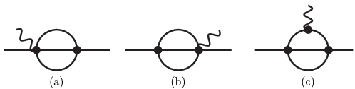
Figure 3: The two-loop diagrams with overlapping loop integrals contributing to the $K_{\ell 3}$ form-factor. A $\bullet$ indicates a vertex from ${\cal L}_{2}$, a $\times$ a vertex from ${\cal L}_{4}$ and a $\otimes$ a vertex from ${\cal L}_{6}$. The insertion of the weak current is indicated by the wiggly line.

The index $i$ in ${\cal L}_{i}$ stands for the chiral power. The precise form of ${\cal L}_{2}$ and ${\cal L}_{4}$ is given below while ${\cal L}_{6}$ can be found in [17]. The lowest order, ${\cal O}(p^{2})$, in the expansion corresponds to tree level diagrams with vertices from ${\cal L}_{2}$, the next-to-leading order, NLO or ${\cal O}(p^{4})$, to one-loop diagrams with vertices from ${\cal L}_{2}$ or tree level diagrams with one vertex from ${\cal L}_{4}$ and the rest from ${\cal L}_{2}$. The next-to-next-to-leading order, NNLO or ${\cal O}(p^{6})$, has two-loop diagrams, one-loop diagrams with one vertex from ${\cal L}_{4}$ and tree level diagrams with one vertex from ${\cal L}_{6}$ or two vertices from ${\cal L}_{4}$ and all other vertices from ${\cal L}_{2}$. The loop diagrams take all singularities due to the Goldstone Bosons correctly into account. The singularities are the real predictions of ChPT while the other effects from QCD are in the values of the LECs. The diagrams, in addition to wave-function-renormalization, relevant for the processes discussed in this paper are shown in Figs. 1, 2 and 3.

The expressions for the first two terms in the expansion of the Lagrangian are given by ($F_{0}$ refers to the pseudoscalar decay constant in the chiral limit)

$${\cal L}_{2}=\frac{F_{0}^{2}}{4}\{\langle D_{\mu}U^{\dagger}D^{\mu}U\rangle+\langle\chi^{\dagger}U+\chi U^{\dagger}\rangle\}\,,$$ (2.2)

and

$${\cal L}_{4} =L_{1}\langle D_{\mu}U^{\dagger}D^{\mu}U\rangle^{2}+L_{2}\langle D_{\mu}U^{\dagger}D_{\nu}U\rangle\langle D^{\mu}U^{\dagger}D^{\nu}U\rangle$$ (2.3)

$$+L_{3}\langle D^{\mu}U^{\dagger}D_{\mu}UD^{\nu}U^{\dagger}D_{\nu}U\rangle+L_{4}\langle D^{\mu}U^{\dagger}D_{\mu}U\rangle\langle\chi^{\dagger}U+\chi U^{\dagger}\rangle$$

$$+L_{5}\langle D^{\mu}U^{\dagger}D_{\mu}U(\chi^{\dagger}U+U^{\dagger}\chi)\rangle+L_{6}\langle\chi^{\dagger}U+\chi U^{\dagger}\rangle^{2}$$

$$+L_{7}\langle\chi^{\dagger}U-\chi U^{\dagger}\rangle^{2}+L_{8}\langle\chi^{\dagger}U\chi^{\dagger}U+\chi U^{\dagger}\chi U^{\dagger}\rangle$$

$$-iL_{9}\langle F^{R}_{\mu\nu}D^{\mu}UD^{\nu}U^{\dagger}+F^{L}_{\mu\nu}D^{\mu}U^{\dagger}D^{\nu}U\rangle+L_{10}\langle U^{\dagger}F^{R}_{\mu\nu}UF^{L\mu\nu}\rangle\,,$$

while the next-to-next-to-leading order is a rather cumbersome expression [17]. The special unitary matrix $U$ contains the Goldstone boson fields

$$U=\exp\left(\frac{i\sqrt{2}}{F_{0}}M\right)\,,\quad M=\left(\begin{array}[]{ccc}\frac{1}{\sqrt{2}}\pi^{0}+\frac{1}{\sqrt{6}}\eta&\pi^{+}&K^{+}\\ \pi^{-}&\frac{-1}{\sqrt{2}}\pi^{0}+\frac{1}{\sqrt{6}}\eta&K^{0}\\ K^{-}&\overline{K^{0}}&\frac{-2}{\sqrt{6}}\eta\end{array}\right)\,.$$ (2.4)

The formalism is the external field method of [18] with $s$, $p$, $l_{\mu}$ and $r_{\mu}$ matrix valued scalar, pseudo-scalar, left-handed and right-handed vector external fields respectively. These show up in

$$\chi=2B_{0}\left(s+ip\right)\,,$$ (2.5)

in the covariant derivative

$$D_{\mu}U=\partial_{\mu}U-ir_{\mu}U+iUl_{\mu}\,,$$ (2.6)

and in the field strength tensor

$$F_{\mu\nu}^{L(R)}=\partial_{\mu}l(r)_{\nu}-\partial_{\nu}l(r)_{\mu}-i\left[l(r)_{\mu},l(r)_{\nu}\right]\,.$$ (2.7)

For our purpose it is sufficient to set

$$s=\left(\begin{array}[]{ccc}\hat{m}&&\\ &\hat{m}&\\ &&m_{s}\end{array}\right)\,,\quad r_{\mu}=0\,,\quad l_{\mu}=-\frac{g_{2}}{\sqrt{2}}\left(\begin{array}[]{ccc}&V_{ud}W^{+}_{\mu}&V_{us}W^{+}_{\mu}\\ V_{ud}^{*}W^{-}_{\mu}&&\\ V_{us}^{*}W^{-}_{\mu}&&\end{array}\right)$$ (2.8)

with $g_{2}$ the weak coupling constant, related to the Fermi constant by

$$\frac{G_{F}}{\sqrt{2}}=\frac{g_{2}^{2}}{8m_{W}^{2}}\,.$$ (2.9)

2.1 Renormalization Scheme

We use the renormalization scheme as explained in [17] and [19]. It extends the scheme from [18] naturally to two-loops. Notice that the work of Post and Schilcher [10, 20, 21] used a slightly different scheme. The scheme employed here does not introduce the $\epsilon^{2}$ term in Eq. (39) of Ref. [10]. Subtractions are performed via

$$L_{i} = (C\mu)^{(d-4)}\left(\Gamma_{i}+L_{i}(\mu)\right)\,,$$

$$C_{i} = (C\mu)^{2(d-4)}\left(C_{i}^{r}(\mu)-\frac{1}{F^{2}}\left[\Gamma_{i}^{(2)}\Lambda^{2}+(\Gamma_{i}^{(1)}+\Gamma_{i}^{(L)}(\mu))\Lambda\right]\right)\,,$$ (2.10)

with

$$\ln C=-\frac{1}{2}\left(\ln(4\pi)+\Gamma^{\prime}(1)+1\right),\quad\Lambda=\frac{1}{16\pi^{2}(d-4)}\,.$$ (2.11)

The coefficients $\Gamma_{i}$ can be found in [18, 17] and the $\Gamma_{i}^{(2)},\Gamma_{i}^{(1)}\Gamma_{i}^{(L)}(\mu)$ in [17]. We will in the remainder always write $C_{i}^{r}$ and $L_{i}^{r}$ but the $\mu$ dependence is of course present.

3 The $K_{\ell 3}$ form-factors: definition and ${\cal O}(p^{4})$

The decays we consider are

$$K^{+}(p) \rightarrow \pi^{0}(p^{\prime})\ell^{+}(p_{\ell})\nu_{\ell}(p_{\nu})\,,\hskip 28.45274pt[K_{\ell 3}^{+}]$$ (3.1)

$$K^{0}(p) \rightarrow \pi^{-}(p^{\prime})\ell^{+}(p_{\ell})\nu_{\ell}(p_{\nu})\,,\hskip 28.45274pt[K_{\ell 3}^{0}]$$ (3.2)

and their charge conjugate modes. $\ell$ stands for $\mu$ or $e$.

The matrix-element for $K_{\ell 3}^{+}$, neglecting scalar and tensor contributions, has the structure

$$T = \frac{G_{F}}{\sqrt{2}}V_{us}^{\star}\ell^{\mu}{F_{\mu}}^{+}(p^{\prime},p)\,,$$ (3.3)

with

$$\ell^{\mu} = \bar{u}(p_{\nu})\gamma^{\mu}(1-\gamma_{5})v(p_{\ell})\,,$$

$${F_{\mu}}^{+}(p^{\prime},p) = <\pi^{0}(p^{\prime})\mid V_{\mu}^{4-i5}(0)\mid K^{+}(p)>\,,$$ (3.4)

$$= \frac{1}{\sqrt{2}}[(p^{\prime}+p)_{\mu}f^{K^{+}\pi^{0}}_{+}(t)+(p-p^{\prime})_{\mu}f_{-}^{K^{+}\pi^{0}}(t)].$$

To obtain the $K_{\ell 3}^{0}$ matrix-element, one replaces $F^{+}_{\mu}$ by

$${F_{\mu}}^{0}(p^{\prime},p) = <\pi^{-}(p^{\prime})\mid V_{\mu}^{4-i5}(0)\mid K^{0}(p)>$$ (3.5)

$$= (p^{\prime}+p)_{\mu}f^{K^{0}\pi^{-}}_{+}(t)+(p-p^{\prime})_{\mu}f_{-}^{K^{0}\pi^{-}}(t).$$

The processes (3.1) and (3.2) thus involve the four $K_{\ell 3}$ form-factors $f^{K^{+}\pi^{0}}_{\pm}(t)$, $f^{K^{0}\pi^{-}}_{\pm}(t)$ which depend on

$$t=(p^{\prime}-p)^{2}=(p_{\ell}+p_{\nu})^{2},$$ (3.6)

the square of the four momentum transfer to the leptons.

In this paper we work in the isospin limit thus

$$f_{\pm}=f_{\pm}^{K\pi}=f_{\pm}^{K^{+}\pi^{0}}=f_{\pm}^{K^{0}\pi^{-}}\,.$$ (3.7)

$f_{+}^{K\pi}$ is referred to as the vector form-factor, because it specifies the $P$-wave projection of the crossed channel matrix-elements $<0\mid V^{4-i5}_{\mu}(0)\mid K^{+},\pi^{0}\;\mbox{in}>$. The $S$-wave projection is described by the scalar form-factor

$$f_{0}(t)=f_{+}(t)+\frac{t}{m^{2}_{K}-m^{2}_{\pi}}f_{-}(t)\,.$$ (3.8)

Analyses of $K_{\ell 3}$ data frequently assume a linear dependence

$$f_{+,0}(t)=f_{+}(0)\left[1+\lambda_{+,0}\frac{t}{m^{2}_{\pi^{+}}}\right]\;\;.$$ (3.9)

For a discussion of the validity of this approximation see [5] and references cited therein. We will discuss it to order $p^{6}$ and in comparison with the data. At the expected future precision it will be necessary to go beyond this approximation.

Eqs. (3.8) and (3.9) leads to a constant $f_{-}(t)$ ,

$$f_{-}(t)=f_{-}(0)=f_{+}(0)(\lambda_{0}-\lambda_{+})\frac{m_{K}^{2}-m_{\pi}^{2}}{m_{\pi^{+}}^{2}}.$$ (3.10)

The form-factors $f_{\pm,0}(t)$ are analytic functions in the complex $t$-plane cut along the positive real axis. The cut starts at $t=(m_{K}+m_{\pi})^{2}$. In our phase convention, the form-factors are real in the physical region

$$m^{2}_{\ell}\leq t\leq(m_{K}-m_{\pi})^{2}.$$ (3.11)

A discussion of the kinematics in $K_{\ell 3}$ decays can be found in [6].

4 Analytical Results

The total result we obtain is split by chiral order.

$$f_{i}(t)=f_{i}^{(2)}(t)+f_{i}^{(4)}(t)+f_{i}^{(6)}(t)\,,\quad(i=+,-,0)\,.$$ (4.1)

4.1 Order $p^{2}$

This has been known for a very long time and is fully determined by gauge invariance.

$$f_{+}^{(2)}(t)=f_{0}^{(2)}(t)=1,,\quad\quad\quad f_{-}^{(2)}(t)=0\,.$$ (4.2)

It results from the diagram in Fig. 1(a).

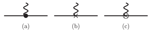
Figure 1: The tree level diagrams contributing to the $K_{\ell 3}$ form-factor. A $\bullet$ indicates a vertex from ${\cal L}_{2}$, a $\times$ a vertex from ${\cal L}_{4}$ and a $\otimes$ a vertex from ${\cal L}_{6}$. The insertion of the weak current is indicated by the wiggly line.

4.2 Order $p^{4}$

This was first calculated within the ChPT framework by Gasser and Leutwyler in 1985 [5]. The result contains the nonanalytic dependence in the symmetry parameters predicted by [22]. The form of the form-factors we use (which is equivalent to the result of [5] to order $p^{4}$) is the one which our expressions for the $p^{6}$ contribution correspond to.

$$F_{\pi}^{2}\,f_{+}^{(4)}(t) = 2L_{9}^{r}t+3/8\left(\overline{A}(m_{\eta}^{2})+\overline{A}(m_{\pi}^{2})+2\overline{A}(m_{K}^{2})\right)$$ (4.3)

$$-3/2\,\left(\overline{B}_{22}(m_{\pi}^{2},m_{K}^{2},t)+\overline{B}_{22}(m_{K}^{2},m_{\eta}^{2},t)\right)\,.$$

$$F_{\pi}^{2}\,f_{-}^{(4)}(t) = (4m_{K}^{2}-4m_{\pi}^{2})L_{5}^{r}-2(m_{K}^{2}-m_{\pi}^{2})L_{9}^{r}+1/2\overline{A}(m_{\eta}^{2})-5/12\overline{A}(m_{\pi}^{2})$$ (4.4)

$$+7/12\overline{A}(m_{K}^{2})+\overline{B}(m_{\pi}^{2},m_{K}^{2},t)(-1/12m_{\pi}^{2}-5/12m_{K}^{2}+5/12t)$$

$$+\overline{B}(m_{K}^{2},m_{\eta}^{2},t)(1/12m_{\pi}^{2}-7/12m_{K}^{2}+1/4t)$$

$$+\overline{B}_{1}(m_{\pi}^{2},m_{K}^{2},t)(-7/12m_{\pi}^{2}+19/12m_{K}^{2}-5/12t)$$

$$+\overline{B}_{1}(m_{K}^{2},m_{\eta}^{2},t)(-11/12m_{\pi}^{2}+23/12m_{K}^{2}-1/4t)$$

$$+\overline{B}_{21}(m_{\pi}^{2},m_{K}^{2},t)(3/2m_{\pi}^{2}-3/2m_{K}^{2}-5/6t)$$

$$+\overline{B}_{21}(m_{K}^{2},m_{\eta}^{2},t)(3/2m_{\pi}^{2}-3/2m_{K}^{2}-1/2t)$$

$$+\overline{B}_{22}(m_{\pi}^{2},m_{K}^{2},t)(-5/6)+\overline{B}_{22}(m_{K}^{2},m_{\eta}^{2},t)(-1/2)\,.$$

These results are obtained from the diagrams in Figs. 1(b), 2(a) and 2(c), together with wave-function renormalization.

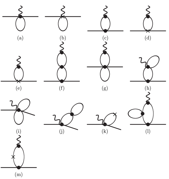
Figure 2: The one and two-loop diagrams without overlapping loop integrals contributing to the $K_{\ell 3}$ form-factor. A $\bullet$ indicates a vertex from ${\cal L}_{2}$, a $\times$ a vertex from ${\cal L}_{4}$ and a $\otimes$ a vertex from ${\cal L}_{6}$. The insertion of the weak current is indicated by the wiggly line.

4.3 Order $p^{6}$

The $p^{6}$ contribution we split in several parts

$$f_{i}^{(6)}(t)=\frac{1}{F_{\pi}^{4}}\left(f_{i}^{C}(t)+f_{i}^{L}(t)+f_{i}^{B}(t)+f_{i}^{H}(t)+f_{i}^{V}(t)\right)\,,\quad(i=+,-,0)\,.$$ (4.5)

The split between the last three terms is not unique and depends on how the irreducible two-loop integrals are separated from the reducible ones. The first two terms are the ones containing the dependence on the $p^{6}$ and $p^{4}$ coupling constants.

The ones with dependence on $C_{i}^{r}$ stem from wave-function renormalization and the diagram of Fig. 1(c). The results are

$$f_{+}^{C}(t) \equiv R_{+0}^{K\pi}+tR_{+1}^{K\pi}+t^{2}R_{+2}^{K\pi}$$ (4.6)

$$= -8\left(m_{\pi}^{2}-m_{K}^{2}\right)^{2}\,\left(C_{12}^{r}+C_{34}^{r}\right)+t\Big{[}-4m_{\pi}^{2}(2C_{12}^{r}+4C_{13}^{r}+C_{64}^{r}$$

$$+C_{65}^{r}+C_{90}^{r})+m_{K}^{2}(-8C_{12}^{r}-32C_{13}^{r}-8C_{63}^{r}-8C_{64}^{r}-4C_{90}^{r})\Big{]}$$

$$+t^{2}(-4C_{88}^{r}+4C_{90}^{r})\,,$$

and

$$f_{-}^{C}(t) \equiv R_{-0}^{K\pi}+tR_{-1}^{K\pi}+t^{2}R_{-2}^{K\pi}$$ (4.7)

$$= \left(m_{K}^{2}-m_{\pi}^{2}\right)\Big{[}m_{\pi}^{2}(+24C_{12}^{r}-16C_{13}^{r}+8C_{15}^{r}+16C_{17}^{r}+8C_{34}^{r}+4C_{64}^{r}$$

$$+4C_{65}^{r}+4C_{90}^{r})+m_{K}^{2}(+24C_{12}^{r}+32C_{13}^{r}+16C_{14}^{r}+16C_{15}^{r}+8C_{34}^{r}$$

$$+4C_{63}^{r}+8C_{64}^{r}+4C_{90}^{r})\Big{]}+t4\left(m_{K}^{2}-m_{\pi}^{2}\right)\left(-2C_{12}^{r}+C_{88}^{r}-C_{90}^{r}\right)\,.$$

We have followed a notation very close to the one in [14]. Notice that we have the relations

$$R_{-2}^{K\pi} = 0\,,$$

$$R_{+2}^{K\pi} = R_{V2}^{\pi}=R_{V2}^{K^{+}}\,,$$

$$R_{+1}^{K\pi} = \frac{1}{2}\left(R_{V1}^{\pi}+R_{V1}^{K^{+}}\right)+R_{V1}^{K^{0}}\,.$$ (4.8)

The other $R_{i}^{M}$ are similar combinations of the $C_{i}^{r}$ but in the expansion of the electromagnetic form-factors [14]. Notice that the last relation is really Sirlin’s relation [23] and the second satisfies it as well.

We have not quoted the remaining formulas, but will quote below some approximate numerical expressions. The exact formulas can be obtained from the authors on request. Our expressions satisfy the Ademollo-Gatto theorem [24].

5 Getting the value of $f_{+}(0)$

One of the problems we face here is whether the needed $C_{i}^{r}$ can be determined from experiment. There are many of these coefficients showing up but as is obvious from Eq. (4.6), what we need is a value for $C_{12}^{r}+C_{34}^{r}$. It turns out that this combination can actually be determined from $K_{\ell 3}$ measurements. The derivation given below relies on the fact that we need values for the $p^{4}$ constants, determined to order $p^{4}$ only, in the order $p^{6}$ part to be correct to the accuracy that we are working. We can determine all needed $L_{i}^{r}$ to this accuracy relying only on data.

We construct the quantity

$$\tilde{f}_{0}(t)=f_{+}(t)+\frac{t}{m_{K}^{2}-m_{\pi}^{2}}\left(f_{-}(t)+1-F_{K}/F_{\pi}\right)=f_{0}(t)+\frac{t}{m_{K}^{2}-m_{\pi}^{2}}\left(1-F_{K}/F_{\pi}\right)\,.$$ (5.1)

This has no dependence on the $L_{i}^{r}$ at order $p^{4}$, only via order $p^{6}$ contributions. Inspection of the dependence on the $C_{i}^{r}$ shows that

$$\tilde{f}_{0}(t) = 1-\frac{8}{F_{\pi}^{4}}\left(C_{12}^{r}+C_{34}^{r}\right)\left(m_{K}^{2}-m_{\pi}^{2}\right)^{2}+8\frac{t}{F_{\pi}^{4}}\left(2C_{12}^{r}+C_{34}^{r}\right)\left(m_{K}^{2}+m_{\pi}^{2}\right)$$ (5.2)

$$-\frac{8}{F_{\pi}^{4}}t^{2}C_{12}^{r}+\overline{\Delta}(t)+\Delta(0)\,.$$

We emphasize that the quantities $\overline{\Delta}(t)$ and $\Delta(0)$ can in principle be calculated to order $p^{6}$ accuracy with knowledge of the $L_{i}^{r}$ to order $p^{4}$ accuracy. In practice, since a $p^{4}$ fit will include in the values of the $L_{i}^{r}$ effects that come from the $p^{6}$ loops (due to the fitting to experimental values) we consider the $p^{6}$ fits to be the relevant ones to avoid double counting effects. Numerical results will be discussed in Section  8.

The definition in (5.1) has essentially used the Dashen-Weinstein relation [25] to remove the $L_{i}^{r}$ dependence at order $p^{4}$. It has also the effect that it removed many of the $C_{i}^{r}$ from the scalar form-factor as well. The corrections which appear in the Dashen-Weinstein relation are include in the functions $\overline{\Delta}(t)$ and $\Delta(0)$, these have both order $p^{4}$ [5, 22] and order $p^{6}$ contributions.

It is obvious from Eq. (5.2) that the needed combination of $C_{i}^{r}$ can be determined from the slope and the curvature of the scalar form-factor in $K_{\ell 3}$ decays.

It seems possible that $C_{12}^{r}$ can be measured from the curvature of the pion scalar form-factor near 0 [26]. When this calculation is complete, one can use the dispersive estimates of the pion scalar form-factor together with only a $\lambda_{0}$ measurement in $K_{\mu 3}$ to obtain the $p^{6}$ value for $f_{+}(0)$. There are also some dispersive estimates for the relevant scalar form-factor. Unfortunately, these are not in a usable form at present [27].

The discussion of Ref. [9] can be shown in this light too. The constant $A_{3}$ of generalized perturbation theory correspond to a combination of the $C_{i}^{r}$ from [17]. The precise combination is

$$A_{3}=(2B_{0})^{2}\left[-C_{34}^{r}+\frac{1}{2}\left(C_{14}^{r}+C_{17}^{r}+C_{26}^{r}+C_{29}^{r}+C_{31}^{r}\right)+\frac{1}{6}C_{33}^{r}\right]\,.$$ (5.3)

As we have shown it is possible to eliminate all but $C_{34}^{r}$, so this plays the role of $A_{3}$ here. $C_{12}^{r}$ is higher order in the counting employed in [9] and was not considered there.

In Ref. [9] the additional observation was made that a relatively small change in the ratio $F_{K}/F_{\pi}$, together with an adjustement of the constant $A_{3}$ can accommodate the CKM unitarity.

6 Data

6.1 $K^{0}_{\mu 3}$

The most useful data points are those where the full dependence on the kinematical variable $t=q^{2}/m_{\pi}^{2}$ is shown. That means that the experiments that determined the value of $\lambda_{0}$ from the branching ratio or did not provide an actual $t$ dependence but just fitted the linear slope in a global way are not that useful for us, but see below.

Of the more recent experiments that quote data not from the branching ratio, the ones that gave a plot or numbers for $f_{0}(t)$ are [28, 29, 30, 31]. Ref. [32] gives a plot but mentions that it is not statistically significant, which inspection of the plots confirms.

There are some obvious problems with the data. E.g. the $f_{0}(t)$ from [28] do not go to 1 at $t=0$. We have shown these data in Fig. 4 together with a linear and a pole approximation corresponding to a mass of 800 MeV. This shows the accuracy needed to see the curvature.

6.2 $K^{+}_{\mu 3}$

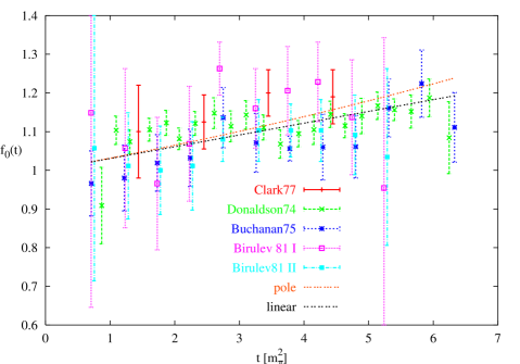
Figure 4: The data on $f_{0}(t)/f_{+}(0)$ from $K^{0}_{\mu 3}$. The data are Clark77 [29], Donaldson74 [28], Buchanan75 [31] and Birulev81 [30], The latter reference has two distinct data sets. For comparison a linear approximation and a pole approximation with a mass of 800 MeV are shown as well.

Here we have not been able to find data that show a plot of $f_{0}(t)$. All experiments are analyzed in terms of a constant form-factor as discussed in [2]. There is one more experiment [33] that quotes measurements of $\lambda_{0}$ not included in [2].

6.3 $K^{0}_{e3}$

Here the data are dominated by the recent high statistics CPLEAR data [34]. There exists a very high statistics older experiment [35]. They provide plots with different data assumptions and can thus not be easily compared at the level of $f_{+}(t)$ directly. But [35] quoted both a linear and quadratic fit to $f_{+}(t)$. In order to show the relation between the most recent and older data we have plotted the data of [31], [30] and [34] in Fig. 5.

We have performed some simple fits of the form

$$f_{+}(t)=a_{+}\left(1+\lambda_{+}\frac{t}{m_{\pi^{+}}^{2}}+c_{+}t^{2}\right)$$ (6.1)

to the CPLEAR data. The fits agree extremely well with those reported in [34] and are given in Table 1.

form	$a_{+}$	$\lambda_{+}$	$c_{+}$	$10^{5}~{}R_{+1}^{K\pi}$	$10^{3}~{}R_{+2}^{K\pi}$
			[GeV-4]	[GeV-2]
Eq. (6.1)	$\equiv 1$	$0.0245\pm 0.0006$	$\equiv 0$
Eq. (6.1)	$1.000\pm 0.004$	$0.0245\pm 0.0015$	$\equiv 0$
Eq. (6.1)	$\equiv 1$	$0.0238\pm 0.0017$	$0.5\pm 1.2$
Eq. (6.1)	$1.008\pm 0.009$	$0.0181\pm 0.0068$	$2.8\pm 2.8$
Eq. (8.2)	$1.008\pm 0.008$	$0.0180\pm 0.0067$	$2.7\pm 3.0$	$-4.3\pm 2.5$	$0.19\pm 0.21$
Eq. (8.2)	$\equiv 1$	$0.0236\pm 0.0019$	$0.4\pm 1.2$	$-2.2\pm 0.7$	$0.02\pm 0.09$
Eq. (8.2)	$\equiv 1$	$0.0201\pm 0.0006$	$3.2$	$-4.7\pm 0.5$	$\equiv 0.22$
Eq. (8.2)	$1.009\pm 0.004$	$0.0170\pm 0.0015$	$3.2$	$-4.7\pm 0.5$	$\equiv 0.22$

Table 1: The fits to the CPLEAR data of various theoretical forms of $f_{+}$. In the last four fits, which use th ChPT results, $\lambda_{+}$ and $c_{+}$ are derived quantities. The symbol $\equiv$ means this quantity was set to this value in the fit.

Notice that the fits that go beyond the linear approximation and leave the normalization free give a significantly lower $\lambda_{+}$ and with larger errors. It is within its errors compatible with the linear fit, but outside the errors from the linear fit, we consider that result from the fit with curvature to be more reliable. The shift is of similar size to that observed in Table 1 in [35].

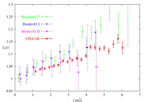
Figure 5: The data on $f_{+}(t)/f_{+}(0)$ from $K^{0}_{e3}$. The CPLEAR data are from Ref. [34]. The older data are for comparison, Buchanan75 is [31] and Birulev81 is [30]. The latter reference has two distinct data sets.

6.4 $K^{+}_{e3}$

There are recent high statistics experiments that show plots of $f_{+}(t)$. They are [36, 37]. We will dicuss the data from [37] below.

6.5 $\lambda_{0}$ and $\lambda_{+}$

Most experiments have analyzed their data assuming linear form-factors. In Table 2 we have quoted the PDG2002 values and the more recent experiments not included in it. We will not use these numbers much, given the possible shifts when introducing a curvature in the analysis.

Process	Ref.	$\lambda_{+}$	$\lambda_{0}$
$K^{+}_{\mu 3}$	[2]	$0.033\pm 0.010$	$0.004\pm 0.009$
$K^{+}_{\ell 3}$	[2]$\mu e$	$0.0282\pm 0.0027$	$0.013\pm 0.005$
$K^{0}_{\mu 3}$	[2]	$0.033\pm 0.005$	$0.027\pm 0.006$
$K^{0}_{\ell 3}$	[2]$\mu e$	$0.0300\pm 0.0020$	$0.030\pm 0.005$
$K^{0}_{e3}$	[2]	$0.0291\pm 0.0018$	–
$K^{+}_{e3}$	[2]	$0.0278\pm 0.0019$	–
$K^{+}_{e3}$	[36]	$0.0293\pm 0.0025$	–
$K^{+}_{\mu 3}$	[33]	$0.0321\pm 0.0045$	$0.0209\pm 0.0045$
$K^{+}_{e3}$	[37]	$0.0278\pm 0.0023$	–
$K^{0}_{e3}$	[38]	$0.02748\pm 0.00084$	–

Table 2: The PDG averages for $\lambda_{+}$ and $\lambda_{0}$ and the values from the most recent experiments. $\mu e$ means that lepton universality has been used in the measurement. The result of [37] is an update of [39] which was included in the PDG averages. The last result [38] is preliminary.

7 Inputs

As relevant combinations we have obtained in our earlier work [14] experimental values for $R_{V2}^{\pi}$ leading to

$$R_{+2}^{K\pi}=(0.22\pm 0.02)~{}\cdot 10^{-3}$$ (7.1)

and

$$L_{9}^{r}=(5.93\pm 0.43)~{}\cdot 10^{-3}$$ (7.2)

which used the estimate $R_{V1}^{\pi}=-0.49~{}\cdot 10^{-5}~{}\mbox{GeV}^{2}$. The two resonance estimates for the $R_{V1}^{M}$ quantities done in [14, 40] via naive vector-meson dominance and the chiral inspired variety lead to basically the same estimate

$$R_{+1}^{K\pi}\approx-4~{}\cdot 10^{-5}~{}\mbox{GeV}^{2}\,.$$ (7.3)

For inputs for the other parameters we use our fits that include the latest $K_{\ell 4}$ data [41]. These are the $p^{4}$ fit, and fit 10 to 13 in Table 2 in [13]. This is a reasonable variation of the various input parameters.

We use the PDG2002 mass values for all the particles involved and

$$F_{\pi}=92.4~{}\mbox{MeV}\,,\quad F_{K}/F_{\pi}=1.22\,.$$ (7.4)

The amplitudes for the decays $K^{+}_{\ell 3}$ are calculated with the mass of the charged kaon and the neutral pion. Those for $K^{0}_{\ell 3}$ with the mass of the neutral kaon and the charged pion.

The scale we use in all the coupling constants and the loop integrals is $\mu=m_{\rho}=700$ MeV. Almost all conclusions are done from experimental determinations of the various parameters so the results are $\mu$-independent.

8 Numerical Results

8.1 Size of the pure loop contributions

In Fig. 6 we show the results from the pure loop diagrams for $f_{+}(t)$. The different lines are for different choices of pion, kaon and eta masses. They give some indication of the size of quark-mass isospin breaking, but it does not include the enhanced effect discussed in [4, 5].

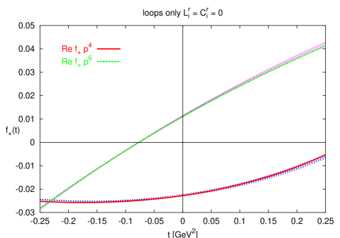
Figure 6: The pure loop diagram contributions to $f_{+}(t)$. Shown are the $p^{4}$ and the $p^{6}$ results for several different choices of the pion, kaon and eta masses.

In Fig. 7 we show the equivalent results for $f_{-}(t)$.

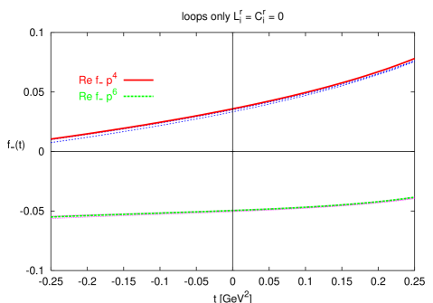
Figure 7: The pure loop diagram contributions to $f_{-}(t)$. Shown are the $p^{4}$ and the $p^{6}$ results for several different choices of the pion, kaon and eta masses.

8.2 Comparison with Refs. [10, 21]

At this point we should also compare with the calculation of [10]. In that paper numerical results are quoted in Eqs. (91-94). We agree, if we use input $L_{i}^{r}$ and masses the same as theirs, well with their numerical expressions for $\Delta^{\mbox{\tiny loop}}_{p^{6}}f_{-}$ (their Eqs. (92) and (94)) and with their numerical value for $\Delta^{\mbox{\tiny loop}}_{p^{6}}f_{+}(0)$ (their Eq. (93)). We do not agree with their expression for the $t$-dependence of $\Delta^{\mbox{\tiny loop}}_{p^{6}}f_{+}$, our numerical values differ by roughly a factor of two. Given the good agreement with the other values this is rather puzzling.

We have attempted to trace the possible sources of discrepancy, and the present conclusions are: i) recalculating with all $L_{i}^{r}=0$ or only $L_{9}^{r}=0$ does not lead to agreement. If we use as input instead $L_{9}^{r}=0.0082$ we get good agreement with $f_{+}(t)$, but it spoils the agreement for $f_{-}(t)$. ii) We have used a different split for the reducible and irreducible parts of the integrals and a different subtraction scheme. Comparing direct subresults is therefore rather difficult. We have also compared our results for the pion electromagnetic form-factor [14] with those in [21]. We have a small discrepancy for the real part there but a rather large discrepancy in the imaginary part. The imaginary part as calculated in [14] would give a phase of a few degrees in [14] while those of [21] give a phase significantly above 10 degrees towards 500 MeV. The latter is not compatible with the expected perturbative buildup of the phase from ChPT. iii) The main expected source of discrepancy is the slightly different renormalization scheme. The quantity we disagree most strongly on has a strong cancellation for the value of the $L_{i}^{r}$ used between the pure loop part and the $L_{i}^{r}$ dependent part, possibly amplifying differences in the result.

8.3 $f_{+}(t)$ and Comparison with the CPLEAR and KEP-PS E246 data

The numerical expression for the $p^{6}$ contribution with the $C_{i}^{r}=0$ and the $L_{i}^{r}$ from fit 10 is

$$\frac{1}{F_{\pi}^{4}}\left(f_{i}^{L}(t)+f_{i}^{B}(t)+f_{i}^{H}(t)+f_{i}^{V}(t)\right)$$ (8.1)

$$= 0.01462+0.0896353t+0.0006313t^{2}+0.3414t^{3}\quad[K^{0}_{\ell 3}]$$

$$= 0.01424+0.0840569t+0.0071463t^{2}+0.3493t^{3}\quad[K^{+}_{\ell 3}]$$

with $t$ expressed in GeV² and it is valid in the range $0\leq t\leq 0.13$ GeV².

We now compare our ChPT expression at order $p^{6}$ to the CPLEAR data [34]. The latter data are normalized to one assuming a linear dependence. It is therefore that the polynomial fits done in Sect. 6.3 added a normalization factor as well. We now perform a fit using the inputs for the $L_{i}^{r}$ from fit 10. The other choices of the $L_{i}^{r}$ give essentially similar results. So we fit the CPLEAR data to

$$f_{+}(t)=\frac{a_{+}}{\Delta(0)}\left(1+f_{+}^{(4)}(t)+f_{+}^{(6)}(t)\right)\,.$$ (8.2)

The effect of $R_{+0}^{K\pi}$ of Eq. (4.6) goes into $a_{+}$ while $R_{+2}^{K\pi}$ gives the $C_{i}^{r}$ part of $c_{+}$ and $R_{+1}^{K\pi}$ gives the $C_{i}^{r}$ part of $\lambda_{+}$ ($c_{+}$ and $\lambda_{+}$ are defined in Eq. (6.1)).

Notice that the fitted value, using the input from the pion electromagnetic form-factor for $R_{+2}^{K\pi}$, gives a value for $R_{+1}^{K\pi}$ in good agreement with the naive expectation. Notice also that the presence of a curvature does change the fitted value of the normalization by a little less than one %. A rather important change due to the inclusion of the curvature is the effect on the value of the slope. Notice that, using the ChPT expression and the curvature as determined from the electromagnetic form-factor leads to

$$\lambda_{+}=0.0170\pm 0.0015\,.$$ (8.3)

This value comes from the ChPT in the following way

$$\lambda_{+}=0.0283(p^{4})+0.0011(\mbox{loops }p^{6})-0.0124(C_{i}^{r})\,.$$ (8.4)

The $p^{6}$ correction is about 30%. The difference with the conclusions on $\lambda_{+}$ of [10] is to a large extent due to their fixing the normalization at one.

The CPLEAR data together with the normalized ChPT result without the $C_{i}^{r}$ contribution, the last fit reported in Table 1 and the linear fit done by the CPLEAR collaboration, is shown in Fig. 8.

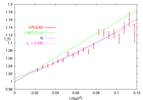
Figure 8: The CPLEAR data together with the normalized ChPT result without the $C_{i}^{r}$, the last fit reported in Table 1 and the linear fit done by the CPLEAR collaboration.

We have performed a similar exercise for the $K^{+}_{e3}$ data from the KEP-PS E246 experiment. This is shown in Fig. 9.

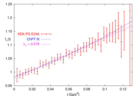
Figure 9: The KEK-PS E246 data together with the ChPT result, with $R_{+1}^{K\pi}$ fitted and the linear fit of the KEK-PS collaboration.

Again, both the linear fit and the one with the curvature fixed from the pion electromagnetic form-factor have a similar $\chi^{2}$. The difference in normalization, relevant for $|V_{us}|$ is about 0.6% and

$$R_{+1}^{K\pi}=-2.5\cdot 10^{-5}\,.$$ (8.5)

The value for $R_{+1}^{K\pi}$ is somewhat different from the value determined from the CPLEAR data, but still compatible with the resonance estimate. The value for the slope is

$$\lambda_{+}=0.0214\pm 0.0018\,.$$ (8.6)

Notice that in both experiments, KEP-PS E-246 and CPLEAR, we have neglected the experimental systematic errors. A possible discrepancy can only be put in after a full experimental analysis is performed. But again, both the normalization and slope are changed significantly from the linear fit case.

8.4 The scalar form-factor $f_{0}(t)$

The scalar form-factor as we have shown above is important since it can be used to determine the $p^{6}$ constants needed to evaluate $f_{+}(0)$. In this section we show numerical results for $f_{0}(t)$ and $\overline{\Delta}(t)$. We have used here the value of $F_{K}/F_{\pi}=1.22$.

In Fig. 10 we show the function $f_{0}(t)-f_{0}(0)$ at order $p^{4}$ and for the various sets of the $L_{i}^{r}$ of Ref. [13]. The value of $f_{0}(0)=f_{+}(0)$ is discussed in the next subsection.

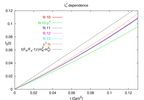
Figure 10: The form-factor $f_{0}(t)-f_{0}(0)$ with the $C_{i}^{r}=0$. Shown are the cases for the neutral kaon decays for various sets of the $L_{i}^{r}$ together with old current algebra result.

As can be seen the convergence from $p^{4}$ to $p^{6}$ is quite good. These are the curves labeled “fit 10 $p^{4}$” and “fit 10”. Notice that all fits of the $L_{i}^{r}$ done at order $p^{6}$ (fit 10-13) give basically identical results. The fit of the $L_{i}^{r}$ at $p^{4}$ (labeled “$p^{4}$ fit”) deviates somewhat but this we consider an artefact as discussed above. For comparison we have shown the part due to $t(1-F_{K}/F_{\pi})/(m_{K}^{2}-m_{\pi}^{2})$.

A good fit over the entire phase space $0\leq t\leq 0.13$ ($t$ in GeV²) is given by

$$\overline{\Delta}(t) = -0.25763t+0.833045t^{2}+1.25252t^{3}\quad[K^{0}_{e3}]$$

$$\overline{\Delta}(t) = -0.260444t+0.846124t^{2}+1.33025t^{3}\quad[K^{+}_{e3}]$$ (8.7)

The error from the values of the different sets of $L_{i}^{r}$ is about 0.0013 at $t=0.13$ GeV².

We have not attempted to do a fit to any of the data given the experimental situation on $\lambda_{0}$. We would however like to point out that the predicted curvature in $f_{0}(t)$ is small but of the same order as in $f_{+}(t)$. As we saw above, this curvature made a rather large change in the measured value of $\lambda_{+}$. A similar effect in $\lambda_{0}$ can thus not be excluded and should be studied experimentally.

8.5 The value of $f_{+}(0)$ and $\Delta(0)$

The results for $f_{+}(0)$ with $C_{i}^{r}=0$ (which is equivalent to $\Delta(0)$) are shown in Table 3. The isospin breaking shown is only an estimate, we have calculated the $K^{+}_{\ell 3}$ case with the masses $m_{K^{+}}$ and $m_{\pi^{0}}$ and $K^{0}_{\ell 3}$ with $m_{K^{0}}$ and $m_{\pi^{+}}$. Further work on including isospin breaking fully to two-loop order is in progress [42].

	$K^{0}_{\ell 3}$	$K^{+}_{\ell 3}$
$p^{4}$	$-0.02266$	$-0.02275$
$p^{6}$ loops only	0.01130	0.01104
$p^{6}$-$L_{i}$ fit 10	0.00332	0.00320
$p^{6}$-$L_{i}$ fit 11	0.00375	0.00355
$p^{6}$-$L_{i}$ fit 12	0.00216	0.00189
$p^{6}$-$L_{i}$ fit 13	0.00539	0.00526
$p^{6}$-$L_{i}$ $p^{4}$ fit	0.00891	0.00863

Table 3: The various contributions to $\Delta(0)=\left.f_{+}(0)\right|_{C_{i}^{r}=0}-1.$

As discussed above, we consider the results with the $L_{i}^{r}$ determined at $p^{4}$ order rather extreme. We have also investigated how $\Delta(0)$ varies if we vary the $L_{i}^{r}$ according to the errors and correlations determined in [13]. For fit 10, the 68% CL error gives 0.00124 and for fit 11 it gives 0.00273. Notice that this latter set allows for a very large variation of $L_{4}^{r}$. We take the latter 0.00273 as a sign of the variation with the $L_{i}^{r}$, notice that includes all the $p^{6}$ fits given above. As a conservative estimate of this error we take half of the $p^{6}$ loop contribution as error and add to it the error from the $L_{i}^{r}$. We thus obtain

$$\Delta(0)=-0.0080\pm 0.0057[\mbox{loops}]\pm 0.0028[L_{i}^{r}]\,.$$ (8.8)

The value of $f_{+}(0)$ is related to $\Delta(0)$ via

$$f_{+}(0)=1+\Delta(0)-\frac{8}{F_{\pi}^{4}}\left(C_{12}^{r}+C_{34}^{r}\right)\left(m_{K}^{2}-m_{\pi}^{2}\right)^{2}\,.$$ (8.9)

A naive estimate of $C_{12}^{r}$ can be made from scalar dominance of the pion scalar form-factor (SMD) leading to

$$\left.C_{12}^{r}\right|_{SMD}=-\frac{F_{\pi}^{4}}{8m_{S}^{4}}\approx-1.0~{}\cdot 10^{-5}\,.$$ (8.10)

The other combination can in principle be estimated from $\lambda_{0}$ via

$$\lambda_{0}=\frac{m_{\pi}^{2}}{m_{K}^{2}-m_{\pi}^{2}}\left(\frac{F_{K}}{F_{\pi}}-1\right)+\frac{8m_{\pi}^{2}}{F_{\pi}^{4}}\left(2C_{12}^{r}+C_{34}^{r}\right)\left(m_{K}^{2}+m_{\pi}^{2}\right)+m_{\pi}^{2}\frac{d}{dt}\overline{\Delta}(t)\,.$$ (8.11)

As an example take $\lambda_{0}=0.009\pm 0.010$ leading to

$$2C_{12}^{r}+C_{34}^{r}=(-1.0\pm 1.7)~{}\cdot 10^{-5}\,.$$ (8.12)

Putting both estimates together gives

$$\left.f_{+}(0)\right|_{C_{i}^{r}}\approx 0.0\pm 0.1.$$ (8.13)

Essentially a $1\%$ precision on $f_{+}(0)$ requires a measurement of $\lambda_{0}$ to 0.001 (about 5%), assuming we can determine $C_{12}^{r}$ with the relevant precision from other sources [26].

The estimate of the $p^{6}$ corrections given in [4] is for the analytic contribution (proportional to $(m_{s}-\hat{m})^{2}$) and contributes to the $C_{i}^{r}$ dependent part

$$\left.f_{+}(0)\right|_{C_{i}^{r}}\approx-0.016\pm 0.008.$$ (8.14)

If we use this value we get for $f_{+}(0)$ the present best estimate

$$f_{+}(0) = 1-0.02266~{}[p^{4}]+0.01130~{}[p^{6}~{}\mbox{pure loops}]+0.00332~{}[p^{6}~{}L_{i}^{r}]-0.016~{}[p^{6}~{}\cite[cite]{[\@@bibref{}{LR}{}{}]}]$$ (8.15)

$$\pm 0.0057[\mbox{loops}]\pm 0.0028~{}[L_{i}^{r}]\pm 0.0080~{}[C_{i}^{r}\cite[cite]{[\@@bibref{}{LR}{}{}]}]$$

$$=\hskip 8.5359pt0.9760\pm 0.0102\,,$$

where errors have been added in quadrature. This satisfies the bound $f_{+}(0)\leq 1$ [43] (as quoted in [4]). Notice that this bound when combined with the other results here gives a constraint on the values of $C_{12}^{r}+C_{34}^{r}$ and thus on a combination of the slope and curvature in the scalar form-factor. The total value and error on $f_{+}(0)$ awaits an experimental determination of the needed constants but Eq. (8.15) is our present best estimate.

The net order $p^{6}$ contribution is roughly one order of magnitude smaller, and with the same sign, as the $p^{4}$ one, due to the sizable cancellation between the calculation of the loop contributions and the estimate of the contribution from the $p^{6}$ constants. We have reevaluated $|V_{us}|$ following the basic steps presented in Sec. 7.3 of [15] but using as input the previous expression (8.15) obtained for the $K^{+}$ decay case. The result should only be taken as preliminary since the full analysis including the isospin breaking terms at $p^{6}$ is still missing as well as an analysis of the effect of the curvature in the form-factor on the experimental value. It explicitly contains: the e.m. corrections at one-loop order and the next-to-next-to-leading order correction in the isospin limit.

$$|V_{us}|=0.2175\pm 0.0029\,,$$ (8.16)

this value is indeed compatible with world-average value $|V_{us}|=0.2196\pm 0.0023$ within errors. Notice that the theoretical errors are larger due to the uncertainty in the $C_{i}^{r}$ and they are at the same footing as the actual experimental ones. Another recent evaluation of $V_{us}$ along the same lines can be found in Ref. [44].

9 Summary and Conclusions

We have performed a calculation to two-loop order of $K_{\ell 3}$ decays in the isospin limit. As far as we have been able to check, this calculation agrees analytically with the earlier on in [10]. We agree with some of the numerical results of that work but not all.

For $K_{\ell 3}$ decay measurements we have shown how the value of $f_{+}(0)$ needed for the determination of $V_{us}$ can be determined from the slope and curvature of $f_{0}(t)$ which can be measured in $K_{\mu 3}$. It is possible that additional information from the pion scalar form-factor near 0 allows the measurement of the slope only to be sufficient [26].

We have presented a present best value for $f_{+}(0)$ based on an estimate of the $p^{6}$ constants $C_{12}^{r}$ and $C_{34}^{r}$. It is clear that this can be further improved after the above measurements are performed. From the calculated best value of $f_{+}(0)$ we can deduce directly an improved estimated value of the CKM matrix element $|V_{us}|$.

As can be seen from our comparison with the data for $f_{+}(t)$ the presence of curvature can make a sizable impact both on the determination of the value of the form-factor at zero and on the slope. The large change in the value $\lambda_{+}$ we found is entirely due to this effect and was compatible with estimates of the $C_{i}^{r}$ involved.

References

- [1] L. M. Chounet, J. M. Gaillard and M. K. Gaillard, Phys. Rept. 4 (1972) 199.
- [2] K. Hagiwara et al. [Particle Data Group Collaboration], Phys. Rev. D 66 (2002) 010001.
- [3] G. Calderon and G. Lopez Castro, Phys. Rev. D 65 (2002) 073032 [hep-ph/0111272].
- [4] H. Leutwyler and M. Roos, Z. Phys. C 25 (1984) 91.
- [5] J. Gasser and H. Leutwyler, Nucl. Phys. B 250 (1985) 517.
- [6] J. Bijnens, G. Colangelo, G. Ecker and J. Gasser, hep-ph/9411311. Published in The second DAPHNE physics handbook, eds. Luciano Maiani, Guilia Pancheri, Nello Paver, 1995.
- [7] J. Bijnens, In 1999 Conference on Kaon Physics, Chicago, IL, USA, 21 - 26 Jun 1999 - Chicago Univ. Press, Chicago, IL, 2001, eds. J. Rosner and B. Winstein, p. 395 hep-ph/9907514.
- [8] J. Bijnens, G. Colangelo and G. Ecker, Phys. Lett. B 441 (1998) 437 [hep-ph/9808421].
- [9] N. H. Fuchs, M. Knecht and J. Stern, Phys. Rev. D 62 (2000) 033003 [hep-ph/0001188].
- [10] P. Post and K. Schilcher, Eur. Phys. J. C 25 (2002) 427 [hep-ph/0112352].
- [11] G. Amorós, J. Bijnens and P. Talavera, Nucl. Phys. B 568 (2000) 319 [hep-ph/9907264].
-
[12]
G. Amorós, J. Bijnens and P. Talavera,
Phys. Lett. B 480 (2000) 71
[hep-ph/9912398];
Nucl. Phys. B 585 (2000) 293 [Erratum-ibid. B 598 (2001) 665] [hep-ph/0003258]. - [13] G. Amorós, J. Bijnens and P. Talavera, Nucl. Phys. B 602 (2001) 87 [hep-ph/0101127].
- [14] J. Bijnens and P. Talavera, JHEP 0203 (2002) 046 [hep-ph/0203049].
- [15] V. Cirigliano, M. Knecht, H. Neufeld, H. Rupertsberger and P. Talavera, Eur. Phys. J. C 23 (2002) 121 [hep-ph/0110153].
-
[16]
Pich, A., Lectures at Les Houches Summer School in
Theoretical Physics, Session 68: Probing the Standard Model of Particle
Interactions, Les Houches, France, 28 Jul - 5 Sep 1997,
[hep-ph/9806303];
Ecker, G., Lectures given at Advanced School on Quantum Chromodynamics (QCD 2000), Benasque, Huesca, Spain, 3-6 Jul 2000, [hep-ph/0011026];
S. Scherer, arXiv:hep-ph/0210398. - [17] J. Bijnens, G. Colangelo and G. Ecker, JHEP 9902 (1999) 020 [hep-ph/9902437].
- [18] J. Gasser and H. Leutwyler, Nucl. Phys. B 250 (1985) 465.
- [19] J. Bijnens, G. Colangelo, G. Ecker, J. Gasser and M. E. Sainio, Nucl. Phys. B 508 (1997) 263 [Erratum-ibid. B 517 (1998) 639] [hep-ph/9707291].
- [20] P. Post and K. Schilcher, Phys. Rev. Lett. 79 (1997) 4088 [hep-ph/9701422].
- [21] P. Post and K. Schilcher, Nucl. Phys. B 599 (2001) 30 [hep-ph/0007095].
- [22] R. F. Dashen, L. Ling-Fong, H. Pagels and M. Weinstein, Phys. Rev. D 6 (1972) 834.
- [23] A. Sirlin, Ann. of Phys. 61 (1970) 294, Phys. Rev. Lett. 43 (1979) 904.
-
[24]
R. E. Behrends and A. Sirlin,
Phys. Rev. Lett. 4 (1960) 186;
M. Ademollo and R. Gatto, Phys. Rev. Lett. 13 (1964) 264. - [25] R. F. Dashen and M. Weinstein, Phys. Rev. Lett. 22 (1969) 1337.
- [26] J. Bijnens and P. Dhonte, “Scalar Form-factors at two-loop in ChPT,” work in preparation.
- [27] M. Jamin, J. A. Oller and A. Pich, Nucl. Phys. B 622 (2002) 279 [arXiv:hep-ph/0110193].
-
[28]
G. Donaldson et al.,
Phys. Rev. D 9 (1974) 2960;
G. Donaldson et al., Phys. Rev. Lett. 31 (1973) 337. - [29] A. R. Clark, R. C. Field, W. R. Holley, R. P. Johnson, L. T. Kerth, R. C. Sah and G. Shen, Phys. Rev. D 15 (1977) 553.
- [30] V. K. Birulev et al., Sov. J. Nucl. Phys. 31 (1980) 622 [Yad. Fiz. 31 (1980) 1204]; V. K. Birulev et al., Nucl. Phys. B 182 (1981) 1.
- [31] C. D. Buchanan et al., Phys. Rev. D 11 (1975) 457.
- [32] D. G. Hill et al., Nucl. Phys. B 153 (1979) 39.
- [33] I. V. Ajinenko et al., Phys. Atom. Nucl. 66 (2003) 105 [Yad. Fiz. 66 (2003) 107] [hep-ph/0202061].
- [34] A. Apostolakis et al. [CPLEAR Collaboration], Phys. Lett. B 473 (2000) 186.
- [35] S. Gjesdal et al., Nucl. Phys. B 109 (1976) 118.
- [36] I. V. Ajinenko et al., Phys. Atom. Nucl. 65 (2002) 2064 [Yad. Fiz. 65 (2002) 2125] [hep-ex/0112023].
- [37] A. S. Levchenko et al. [KEK-PS E246 Collaboration], Phys. Atom. Nucl. 65 (2002) 2232 [Yad. Fiz. 65 (2002) 2294] [hep-ex/0111048].
- [38] R. J. Tesarek [KTeV Collaboration], [KTeV Collaboration] Talk given at American Physical Society (APS) Meeting of the Division of Particles and Fields (DPF 99), Los Angeles, CA, 5-9 Jan 1999. hep-ex/9903069.
- [39] S. Shimizu et al. [KEK-E246 Collaboration], Phys. Lett. B 495 (2000) 33.
- [40] J. Bijnens, G. Colangelo and P. Talavera, JHEP 9805 (1998) 014 [hep-ph/9805389].
- [41] S. Pislak et al. [BNL-E865 Collaboration], Phys. Rev. Lett. 87 (2001) 221801 [hep-ex/0106071].
- [42] J. Bijnens and P. Talavera, work in progress.
- [43] G. Furlan et al., Nuovo Cimento 38 (1965) 1747.
- [44] V. Cirigliano, Talk given at 38th Rencontres de Moriond on Electroweak Interactions and Unified Theories, Les Arcs, France, 15-22 Mar 2003, arXiv:hep-ph/0305154.
- [45] J. A. Vermaseren, math-ph/0010025.