Investigating the Drell-Yan transverse momentum distribution in the color dipole approach

Abstract

Abstract

We study the influence of unitarity corrections on the Drell-Yan transverse momentum distribution within the color dipole approach. These unitarity corrections are implemented through the multiple scattering Glauber-Mueller approach, which is contrasted with a phenomenological saturation model. The process is analyzed for the center of mass energies of the Relativistic Heavy Ion Collider (RHIC, $\sqrt{s}=500$ GeV) and of the Large Hadron Collider (LHC, $\sqrt{s}=14$ TeV). In addition, the results are extrapolated down to current energies of proton-proton collisions, where non-asymptotic corrections to the dipole approach are needed. It is also shown that in the absence of saturation, the dipole approach can be related to the QCD Compton process.

I Introduction

The high energies available in the hadronic reactions at RHIC (BNL Relativistic Heavy Ion Collider) and to be reached at LHC (CERN Large Hadron Collider) will provide a better knowledge concerning parton saturation. In such a kinematical region the production of massive lepton pairs in hadronic collisions (Drell-Yan (DY) process originalDY ) can be used to investigate the high parton density limit, since it is a clean reaction probing the gluon distribution through the QCD Compton process. In particular, the Drell-Yan transverse momentum ($p_{T}$) distribution can be expected to be sensitive to saturation effects.

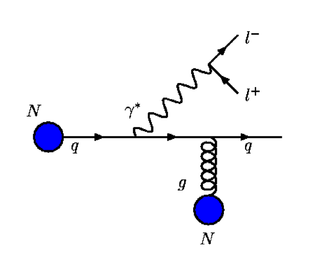
Saturation and nuclear effects are most conveniently described within the color dipole approach DYdipole2 , which is, in fact, especially suitable for this purpose (see Refs. PRD66 ; NuclRauf ; ptprc59 ; GelisJamal for some applications). The dipole approach is applicable only at high energies, and it is formulated in the target rest frame, where the DY process looks like a bremsstrahlung of a virtual photon decaying into a lepton pair (see Fig. 1).

Figure 1: In the target rest frame, DY dilepton production looks like a bremsstrahlung. A quark or an anti-quark from the projectile hadron scatters off the target color field (denoted by a curly line) and radiates a photon ($\gamma^{*}$) with mass $M$ (before or after the quark scatters), which subsequently decays into the lepton pair ($l^{+}l^{-}$).

The advantage of this formalism is that the DY cross section can be written in terms of the same color dipole cross section as small-$x$ Deep Inelastic Scattering (DIS). Although diagrammatically no dipole is present in bremsstrahlung, the dipole cross section arises from the interference of the two bremsstrahlung diagrams, see Ref. PRDrauf for a detailed derivation. The cross section for a radiation of a virtual photon from a quark scattering on a nucleon ($N$) can be written in a factorized form as DYdipole2 ,

$$\frac{d\,\sigma_{T,L}(qN\to\gamma^{*}X)}{d\ln\alpha}=\int\,d^{2}r_{\perp}\,|\Psi^{T,L}_{\gamma^{*}q}(\alpha,r_{\perp})|^{2}\,\sigma_{dip}(\alpha r_{\perp}),$$ (1)

where $\sigma_{dip}$ is the same dipole cross section as in DIS, which should take into account non-perturbative and saturation effects at high energy PRD66 . The energy dependence of $\sigma_{dip}$ is not explicitly written out. Here, $r_{\perp}$ is the photon-quark transverse separation, and the argument of the dipole cross section, $\alpha r_{\perp}$, is the displacement of the projectile quark in impact parameter space due to the radiation of the virtual photon, different to the DIS case, where the dipole separation is just $r_{\perp}$. The $\Psi^{T,L}_{\gamma^{*}q}$ are the light-cone wave functions for radiation of a transversely ($T$) or longitudinally ($L$) polarized photon (see e.g. Ref. PRDrauf for explicit expressions). While the light-cone wave functions are calculable in perturbation theory, the dipole cross section can be determined only with input from experimental data.

The goal of this work is to investigate the influence of unitarity corrections on the DY dilepton $p_{T}$ distribution, describing these unitarity corrections by the multiple scattering Glauber-Mueller approach AGL and including them into the dipole cross section. The results are contrasted with the QCD improved phenomenological saturation model of $\sigma_{dip}$, Ref. newGBW , which quite successfully describes DIS and diffractive DIS data. In lines of a previous work PRD66 , here it is investigated the role of the $\gamma^{*}q$ wave functions in the $p_{T}$ distribution, characterizing the relation between dipole sizes and transverse momentum. A striking advantage of the color dipole picture is a finite cross section for the lepton pair $p_{T}$ distribution at small $p_{T}\to 0$, even in the leading order calculation, feature associated with the saturation encoded in the dipole cross section. In the conventional parton model, the perturbative calculation of ${\cal O}(\alpha_{s})$ yields a divergence at $p_{T}=0$, and one has to resume large logarithms, $\ln\,(p_{T}^{2}/M^{2})$, in an appropriated scheme cososte , in order to obtain a physically sensible result.

The large amount of low Bjorken-$x$ DIS available data allows to constrain the dipole cross section at very high energies and to calculate the DY cross section without additional free parameters. However, in the current energies of the hadronic colliders there are non-asymptotic corrections to the dipole cross section, which have to be taken into account, in order to describe experimental data. Therefore, one also introduces a parameterization for that contribution, which is negligible already at RHIC energies. In addition, we show how the dipole approach for the DY $p_{T}$ distribution is related to the QCD Compton process, which contributes at order $\alpha_{s}$ to the conventional parton model of DY dilepton production. The two approaches are equivalent in a certain limit.

II Relating dipole approach and parton model of high $p_{T}$ dilepton production

Although the dipole approach and the next-to-leading order (NLO) parton model have been compared numerically in Ref. PRDrauf , one may still wonder, how these two approaches can be related to one another analytically. This will be the topic of the present section. Using the leading order expression fs ,

$$\sigma_{dip}(x,r_{\perp})=\frac{\pi^{2}\,\alpha_{s}}{3}\,\,r_{\perp}^{2}\,x\,G(x)\,,$$ (2)

for the dipole cross section, it can be demonstrated how the dipole approach for high $p_{T}$ dilepton production is related to the QCD Compton process, see Fig. 2. In Eq. (2), $x\,G(x)$ is the density of gluons with momentum fraction $x$ in a nucleon, and $\alpha_{s}$ is the strong coupling constant. First, we shortly review the formulas for high $p_{T}$ dilepton production in the dipole approach and in the parton model, before we show how they can be translated into each other.

Figure 2: Production of massive photons through the QCD Compton process. The subsequent decay of the $\gamma^{*}$ (wavy line) into the dilepton pair is not shown here. Curly lines denote gluons, quarks are represented by lines with arrows.

In the dipole approach, the DY transverse momentum distribution is given by RaufThesis ,

$$\frac{d^{3}\sigma(pp\to l^{+}l^{-}X)}{dydM^{2}dp_{T}^{2}}$$ (3)

$$= \frac{\alpha_{em}}{3M^{2}}x_{1}\int\limits_{x_{1}}^{\alpha_{max}}\frac{d\alpha}{\alpha^{2}}\sum\limits_{q=1}^{N_{f}}e_{q}^{2}\left[q\left(\frac{x_{1}}{\alpha}\right)+\bar{q}\left(\frac{x_{1}}{\alpha}\right)\right]$$

$$\times \int d^{2}r_{\perp}d^{2}r^{\prime}_{\perp}e^{i\vec{p}_{T}\cdot\left(\vec{r}_{\perp}-\vec{r}^{\prime}_{\perp}\right)}\left[\Psi^{T}_{\gamma^{*}q}(\alpha,r_{\perp})\Psi^{T*}_{\gamma^{*}q}(\alpha,r^{\prime}_{\perp})+\Psi^{L}_{\gamma^{*}q}(\alpha,r_{\perp})\Psi^{L*}_{\gamma^{*}q}(\alpha,r^{\prime}_{\perp})\right]$$

$$\times \frac{1}{2}\left[\sigma_{dip}(x,\alpha r_{\perp})+\sigma_{dip}(x,\alpha r^{\prime}_{\perp})-\sigma_{dip}(x,\alpha\left|\vec{r}_{\perp}-\vec{r}^{\prime}_{\perp}\right|)\right],$$

where the quark (antiquark) distributions in the projectile are denoted by $q$ ($\bar{q}$ respectively). The usual definitions of the kinematic variables are employed, i.e.,

$$x_{1}=\frac{2P_{2}\cdot q}{s}\quad,\quad x_{2}=\frac{2P_{1}\cdot q}{s},$$ (4)

where $q$ is the four momentum of the virtual photon ($M^{2}=q^{2}$), and $P_{1,2}$ are the four momenta of the projectile ($1$) and target ($2$) hadron. By evaluating the scalar product for $x_{1}$ in the target rest frame, it is easy to show, that the projectile parton distributions in Eq. (3) are probed at momentum fraction $x_{1}/\alpha$, where $\alpha$ is the momentum fraction taken by the photon from the projectile quark. Furthermore, $p_{T}$ is the transverse momentum of the $\gamma^{*}$ in a frame with the $z$-axis parallel to the projectile  quark, and

$$y=\frac{1}{2}\ln\left(\frac{x_{1}}{x_{2}}\right)$$ (5)

is the rapidity of the photon. In addition,

$$\eta^{2}=\left(1-\alpha\right)M^{2}+\alpha^{2}m_{q}^{2}.$$ (6)

The quark mass $m_{q}$ is set to 0 in this section. The upper limit of the $\alpha$-integration in Eq. (3) is determined from the condition that the invariant mass of the final state cannot exceed the total available center of mass (c.m.) energy of the projectile quark-target nucleon system, i.e.,

$$\frac{x_{1}s}{\alpha}\geq\frac{p_{T}^{2}+\eta^{2}}{\alpha\left(1-\alpha\right)}\quad\rightarrow\quad\alpha_{max}=1-\frac{p_{T}^{2}}{x_{1}s-M^{2}},$$ (7)

where $\sqrt{s}$ is the hadronic c.m. energy. In the high energy approximation, $\alpha_{max}=1$ for $s\to\infty$. In this section, however, we work with the exact value of $\alpha_{max}$.

With $\sigma_{dip}$ given by Eq. (2), the integrals over $r_{\perp}$ and $r^{\prime}_{\perp}$ in Eq. (3) can be performed analytically with the result RaufThesis ,

$$\left(\frac{d^{3}\sigma(pp\to l^{+}l^{-}X)}{dydM^{2}dp_{T}^{2}}\right)_{r^{2}_{\perp}-{\rm approx.}}$$ (8)

$$= \frac{\alpha^{2}_{em}\alpha_{s}}{9M^{2}}x_{1}\int\limits_{x_{1}}^{\alpha_{max}}d\alpha\sum\limits_{q=1}^{N_{f}}e_{q}^{2}\left[q\left(\frac{x_{1}}{\alpha}\right)+\bar{q}\left(\frac{x_{1}}{\alpha}\right)\right]xG(x)$$

$$\times \left\{\left[1+\left(1-\alpha\right)^{2}\right]\frac{p_{T}^{4}+\eta^{4}}{\left(p_{T}^{2}+\eta^{2}\right)^{4}}+4M^{2}\left(1-\alpha\right)^{2}\frac{p_{T}^{2}}{\left(p_{T}^{2}+\eta^{2}\right)^{4}}\right\}.$$

In order to obtain Eq. (8), one has to assume that $xG(x)$ does not depend on $r_{\perp}$ through scaling violations. Note also, that the $r^{2}_{\perp}$-approximation, Eq. (2), is applicable only at large $p_{T}$.

In the parton model, on the other hand, the high $p_{T}$ distribution of DY dileptons produced via the QCD Compton process, see Fig. 2, is given by

$$\left(\frac{d^{3}\sigma(pp\to l^{+}l^{-}X)}{dydM^{2}dp_{T}^{2}}\right)_{{\rm Compton}}$$ (9)

$$= \frac{\alpha^{2}_{em}\alpha_{s}}{9M^{2}}\int\limits_{x_{a}^{min}}^{1}dx_{a}\frac{x_{a}x_{b}}{x_{a}-x_{1}}\sum\limits_{q=1}^{N_{f}}e_{q}^{2}\left\{\left[q\left(x_{a}\right)+\bar{q}\left(x_{a}\right)\right]G(x_{b})+G(x_{a})\left[q\left(x_{b}\right)+\bar{q}\left(x_{b}\right)\right]\right\}$$

$$\times \frac{1}{\hat{s}^{2}}\left[-2M^{2}\frac{\hat{t}}{\hat{s}\hat{u}}-\frac{\hat{s}}{\hat{u}}-\frac{\hat{u}}{\hat{s}}\right]$$

(see e.g. Ref. field for details). In Eq. (9), $x_{a}$ and $x_{b}$ are the momentum fractions of the colliding partons, and

$$x_{a}^{min}=\frac{x_{1}-M^{2}/s}{1-x_{2}}.$$ (10)

Note that at finite $p_{T}$, $x_{a,b}\neq x_{1,2}$, where $x_{1,2}=\sqrt{\frac{p_{T}^{2}+M^{2}}{s}}e^{(+,-)y}$. The partonic Mandelstam variables, ${\hat{s}}$, ${\hat{t}}$, ${\hat{u}}$, are defined in terms of $x_{a}$, $x_{b}$ and the four-momenta of the colliding hadrons, see Fig. 2. In order to compare Eqs. (8) and (9), one has to express the partonic Mandelstam variables in terms of $\alpha$ and $p_{T}^{2}$,

$$\hat{s}=\left(x_{a}P_{1}+x_{b}P_{2}\right)^{2} = \frac{p_{T}^{2}+\eta^{2}}{\alpha\left(1-\alpha\right)},$$ (11)

$$\hat{t}=\left(q-x_{b}P_{2}\right)^{2} = -\frac{p_{T}^{2}}{1-\alpha},$$ (12)

$$\hat{u}=\left(q-x_{a}P_{1}\right)^{2} = -\frac{p_{T}^{2}+\eta^{2}}{\alpha}.$$ (13)

Furthermore,

$$x_{a}=\frac{x_{1}}{\alpha}\quad,\quad x_{b}=\frac{p_{T}^{2}+\eta^{2}}{\left(1-\alpha\right)p_{T}^{2}+\eta^{2}}\,x_{2}.$$ (14)

Inserting the expressions for the partonic Mandelstam variables, Eqs. (11), (12) and (13), into Eq. (9), one obtains a result very similar to Eq. (8), except for the combinations of parton distributions,

$$\left(\frac{d^{3}\sigma(pp\to l^{+}l^{-}X)}{dydM^{2}dp_{T}^{2}}\right)_{{\rm Compton}}$$ (15)

$$= \frac{\alpha^{2}_{em}\alpha_{s}}{9M^{2}}x_{1}\int\limits_{x_{1}}^{\alpha_{max}}d\alpha\sum\limits_{q=1}^{N_{f}}e_{q}^{2}\left\{\left[q\left(x_{a}\right)+\bar{q}\left(x_{a}\right)\right]x_{b}G(x_{b})+G(x_{a})x_{b}\left[q\left(x_{b}\right)+\bar{q}\left(x_{b}\right)\right]\right\}$$

$$\times \left\{\left[1+\left(1-\alpha\right)^{2}\right]\frac{p_{T}^{4}+\eta^{4}}{\left(p_{T}^{2}+\eta^{2}\right)^{4}}+4M^{2}\left(1-\alpha\right)^{2}\frac{p_{T}^{2}}{\left(p_{T}^{2}+\eta^{2}\right)^{4}}\right\}.$$

When saturation effects are neglected, the dipole approach reproduces that part of the QCD Compton contribution to DY, in which the quark comes from the projectile and the gluon from the target. Thus, the dipole approach is valid, when the first term in the convolution of parton distributions in Eq. (15) dominates. This is the case at large rapidity and at small $x_{b}$, both conditions fulfilled. The range of validity of the dipole approach can of course only be established a posteriori. This is similar to the problem of determining the lowest scale at which perturbative QCD still works. The dipole approach is phenomenologically successful for values of $x_{2}<0.1$, though most parameterizations of the dipole cross section are fitted only to DIS data with Bjorken-$x<0.01$.

Regarding the rapidity ($y$) range, in which the dipole formulation can be applied, some guidance on the minimal value of $y$ can be obtained from the numerical comparison of the dipole approach and the next-to-leading order (NLO) parton model in Ref. PRDrauf . At RHIC energy $\sqrt{s}=500$ GeV, virtually no deviations between the dipole approach and the NLO parton model have been found for $y>0.5$ PRDrauf . This means that one can safely compare the dipole approach to future DY measurements from the two PHENIX muon arms phenix .

On the other hand, the dipole approach takes into account several effects that will be important at high energies. A realistic parameterization of the dipole cross section includes gluon saturation, which is not contained in the standard parton model. Moreover, $\sigma_{dip}$ contains information about the transverse momentum distribution of the target gluons, thereby is more complete than the gluon distribution in the collinear factorization approach. Finally, with a realistic parameterization of the dipole cross section at large separation $r_{\perp}$, one can apply Eq. (3) also at low $p_{T}$, while the conventional parton model $p_{T}$ distribution, Eq. (9), is applicable only at very high $p_{T}\mathrel{\hbox to0.0pt{\lower 4.0pt\hbox{\hskip 1.0pt$\sim$}\hss}\raise 1.0pt\hbox{$>$}}M$.

III Features of the Drell-Yan cross section in the color dipole approach

In this section, it is investigated which distances $r_{\perp}$ in impact parameter space are important for the Drell-Yan $p_{T}$ distribution. For this purpose, the behavior of the weight function for $\sigma_{dip}$ as function of $\rho=\alpha r_{\perp}$ for different values of $p_{T}$ is studied.

Three of the four Fourier integrals in Eq. (3) can be performed analytically with the result NuclRauf ,

$$\frac{d\,\sigma^{DY}}{dM^{2}\,dx_{F}\,d^{2}p_{T}}=\frac{\alpha^{2}_{\rm{em}}}{6\,\pi^{3}M^{2}}\,\frac{1}{(x_{1}+x_{2})}\int_{0}^{\infty}d\rho W(\rho,p_{T})\sigma_{dip}(\rho),$$ (16)

where the weight function $W(\rho,p_{T})$ is given by

$$W(\rho,p_{T}) = \int_{x_{1}}^{1}\frac{d\alpha}{\alpha^{2}}\,\frac{x_{1}}{\alpha}\sum\limits_{q=1}^{N_{f}}e_{q}^{2}\left[q\left(\frac{x_{1}}{\alpha},M^{2}\right)+\bar{q}\left(\frac{x_{1}}{\alpha},M^{2}\right)\right]$$ (17)

$$\times \left\{[m_{q}^{2}\alpha^{4}+2M^{2}(1-\alpha)^{2}]\left[\frac{1}{p_{T}^{2}+\eta^{2}}T_{1}(\rho)-\frac{1}{4\eta}T_{2}(\rho)\right]\right.$$

$$\left.+\,\,[1+(1-\alpha)^{2}]\left[\frac{\eta p_{T}}{p_{T}^{2}+\eta^{2}}T_{3}(\rho)-\frac{T_{1}(\rho)}{2}+\frac{\eta}{4}T_{2}(\rho)\right]\right\}\,,$$

and the functions $T_{i}$ read,

$$T_{1}(\rho) = \rho J_{0}(p_{T}\rho/\alpha)K_{0}(\eta\rho/\alpha)/\alpha\,,$$ (18)

$$T_{2}(\rho) = \rho^{2}J_{0}(p_{T}\rho/\alpha)K_{1}(\eta\rho/\alpha)/\alpha^{2}\,,$$ (19)

$$T_{3}(\rho) = \rho J_{1}(p_{T}\rho/\alpha)K_{1}(\eta\rho/\alpha)/\alpha\,.$$ (20)

The functions $J_{0}$ and $J_{1}$ are the first class Bessel functions of order $0$ and $1$, whereas $K_{0}$ and $K_{1}$ are the second class modified Bessel functions of order $0$ and $1$ (MacDonald functions).

It was shown in Ref. PRD66 that for the ($p_{T}$ integrated) mass distribution, the wave functions select the small $\rho$ region. Large values of $\rho\mathrel{\hbox to0.0pt{\lower 4.0pt\hbox{\hskip 1.0pt$\sim$}\hss}\raise 1.0pt\hbox{$>$}}2/M$ are exponentiated by the functions $K_{0,1}$. It should be stressed here that large dipole sizes correspond to the non-perturbative sector of the reactions, whereas small size configurations give the perturbative piece.

In the particular case of the dilepton $p_{T}$ distribution, a different picture is designed. In Fig. 3, we show $W(\rho,p_{T})$ as a function of the photon-quark transverse separation $\rho$ for typical fixed lepton pair mass $M=6.5$ GeV and Feynman-$x$ ($x_{F}=0.625$). The results are presented for two center of mass energies: the plot on the left corresponds to $\sqrt{s}=38.8$ GeV (available at the E772), whereas in the plot on the right, $\sqrt{s}=500$ GeV (RHIC). For the effective light quark masses, the value $m_{q}=0.2$ GeV was used. Three different values for the dilepton transverse momentum were selected, $p_{T}=0$, 1 and 4 GeV.

Figure 3: The weight function $W(\rho,p_{T})$ as a function of $\rho$ for different $p_{T}$ at fixed $x_{F}=0.625$ and $M=6.5$ GeV.

As can be seen from Eq. (17), the oscillating Bessel functions $J_{i}$ drive the behavior of the $W(\rho,p_{T})$ as a function of $\rho$. The following general picture can be drawn from the plots: for large $p_{T}$ the large dipole size configurations get suppressed, because $W(\rho,p_{T})$ is rapidly oscillating. This suppression mechanism is different from the exponential suppression of large dipole sizes in the case of the $p_{T}$ integrated cross section, and complicates the numerical calculation of the $p_{T}$ distribution. On the other hand, as $p_{T}$ decreases, large $\rho$ configurations become more important. The case $p_{T}=0$ is of particular interest, since the weight function $W(\rho,p_{T})$ selects very large dipole configurations and such a region is enhanced by increasing the energy. Therefore, the non-perturbative sector of the process should drive the small $p_{T}$ regime. On the other hand, the large $p_{T}$ behavior is almost completely dominated by small dipole configurations Kop1 . These features are exploited in the next section, where are also discussed the different models that were employed for the dipole cross section.

IV The dipole cross section

The cross section for a small color dipole scattering on a nucleon can be obtained from perturbative QCD fs . However, there are large uncertainties stemming from non-perturbative effects (infrared region) as well as from higher order and higher twist corrections. In the leading $\ln(1/x)$ approximation, the dipole interacts with the target through the exchange of a perturbative Balitsky-Fadin-Kuraev-Lipatov (BFKL) Pomeron, described in terms of the ladder diagrams BFKL . In the double logarithmic approximation, the BFKL equation BFKL agrees with the evolution equation of Dokshitzer et al.  DGLAP (hereafter DGLAP equation). In this limit, the dipole cross section reads,

$$\sigma_{dip}(x,r_{\perp})=\frac{\pi^{2}\,\alpha_{s}}{3}\,\,r_{\perp}^{2}\,x\,G^{\mathrm{DGLAP}}(x,\tilde{Q}^{2})\,,$$ (21)

where $xG^{\mathrm{DGLAP}}(x,\tilde{Q}^{2})$ is the usual DGLAP gluon distribution at momentum fraction $x$ and virtuality scale $\tilde{Q}^{2}=\lambda/r_{\perp}^{2}$. The factor $\lambda$ appearing in the virtuality scale $\tilde{Q}^{2}=\lambda/r_{\perp}^{2}$, has been taken as $\lambda=4$ PRD66 , although same magnitude values are equivalent at leading logarithmic level McDermott . The main feature of the dipole cross section above is the color transparency property, i.e., $\sigma_{dip}\sim r_{\perp}^{2}$ as $r_{\perp}\rightarrow 0$. At large dipole size, the dipole cross section should match the confinement property $\sigma_{dip}\sim\sigma_{0}$. Concerning the large transverse separation (non-perturbative sector), our procedure is to freeze the $r^{2}_{\perp}$ in Eq. (21) at a suitable scale larger than $r^{2}_{\mathrm{cut}}$, which corresponds to the initial scale on the gluon density perturbative evolution, $Q^{2}_{0}=4/r^{2}_{\mathrm{cut}}$.

At high energies, an additional requirement should be met: the growth of the parton density (mostly gluons) has to be tamed, since an uncontrolled increasing would violate the Froissart-Martin bound, requiring the black disc limit of the target has to be reached at quite small Bjorken $x$. This feature can be implemented by using the multiple scattering Glauber-Mueller approach (GM), which reduces the growth of the gluon distribution by eikonalization in impact parameter space AGL . Therefore, one substitutes $xG^{\mathrm{DGLAP}}$ in Eq. (21) by the corrected distribution including unitarity effects, $x\,G^{GM}$. A more extensive derivation of the GM dipole cross section and the expression of $x\,G^{GM}$ can be found in the Sec. III of the Ref. PRD66 . Following previous work PRD66 , one shall use $x=x_{2}$ as the energy scale in the dipole cross section, since $x_{2}$ in DY is the analog of Bjorken-$x$ in DIS. Note that $x=\alpha x_{2}$ was used in PRDrauf , however, the factor $\alpha$ has only a small numerical influence.

Once the dipole cross section is known, one can also calculate the DY differential cross section, Eq. (16) integrated over $p_{T}$, and compare it with the available data at small $x_{2}$. However, the current data on DY reactions are measured in a kinematical region where $x_{2}$ still takes rather large values, that is, $x_{2}\simeq 0.1$ at $\sqrt{s}=38.8$ GeV, where the color dipole picture reaches the limit of its validity. Therefore, in order to compare the theory with these data, some procedure should be taken to extend the applicability of the dipole cross section at large $x_{2}$.

Note, that the dipole cross section Eq. (21) represents the asymptotic gluonic (Pomeron) contribution to the process, and at large $x$ (low energy) a non-asymptotic quark-like content should be included. In the Regge theory language, this means a Reggeon contribution, and therefore, we added the term PRD66 ,

$$\sigma^{I\!\!R}_{dip}=\sigma_{0}\,r_{\perp}^{2}\,x^{\,0.425}\,(1-x)^{3}\,.$$ (22)

to the dipole cross section, Eq. (21).

Using the expression above, good results are obtained in describing the E772 data E772 on mass distribution with a Reggeon overall normalization $\sigma_{0}=8$ PRD66 , reproducing similar results considering the saturation model Kop1 . Nevertheless, Eq. (22) has a shortcoming when one calculates the dilepton $p_{T}$ distribution: due to the fact that the weight function, Eq. (17), selects large dipole configurations at small $p_{T}$ (see discussion in the previous section) the $\sim r_{\perp}^{2}$ behavior in the Reggeon dipole cross section produces a non-negligible contribution at small $p_{T}$ even at RHIC energies. Therefore, Eq. (22) was modified in order to cure this shortcoming and preserve our previous results. The Reggeon contribution now reads,

$$\sigma^{I\!\!R}_{dip}=\sigma_{0}\,r_{\perp}^{2}\,x\,q_{\mathrm{val}}\,(x,\tilde{Q}^{2})\,,$$ (23)

where the quantity $q_{\mathrm{val}}$ is the valence quark distribution from the target and a reasonable description of the same E772 data is obtained with a value $\sigma_{0}=7$. The scaling violation from the valence parton distribution takes care of the steep growing on $r_{\perp}$, which is present in the simple parameterization of Eq. (22), removing the already mentioned shortcoming in the $p_{T}$ distribution at high energies. .

Our main goal here is to investigate the DY $p_{T}$ distribution, using the GM dipole cross section. However, for sake of comparison, this analysis is contrasted with the phenomenological saturation model of Bartels et al. (BGBK dipole cross section hereafter), Ref. newGBW , which also includes the features of the dipole cross section discussed above. The model of Ref. newGBW is a QCD improved version of the saturation model of Ref. GBW . The new model explicitly includes QCD evolution, and the dipole cross section is given by,

$$\sigma_{dip}(x,r_{\perp})=\sigma_{0}\left\{1-\exp\left(-\frac{\pi^{2}r^{2}_{\perp}\alpha_{s}(\mu^{2})xg(x,\mu^{2})}{3\sigma_{0}}\right)\right\}\,,$$ (24)

where the scale $\mu^{2}$ is assumed to have the form

$$\mu^{2}=\frac{C}{r^{2}_{\perp}}+\mu_{0}^{2}.$$ (25)

The authors of Ref. newGBW propose the following gluon distribution at initial scale $Q_{0}^{2}=1$ GeV²,

$$xg(x,Q_{0}^{2})=A_{g}x^{-\lambda_{g}}(1-x)^{5.6}.$$ (26)

Altogether, there are five free parameters ($\sigma_{0}$, $C$, $\mu_{0}^{2}$, $A_{g}$ and $\lambda_{g}$), which have been determined in Ref. newGBW by fitting ZEUS, H1 and E665 data with $x<0.01$. In this fit the parameter $\sigma_{0}$ is fixed at 23 mb during the fits as in the original model, Ref. GBW . Here, we employ fit 1 of Ref. newGBW .

In Ref. PRDrauf , where the old saturation model of Ref. GBW was used, the dipole approach was extrapolated to larger $x_{2}$ by introducing a threshold factor into the saturation scale, i.e. $Q^{2}_{s}\rightarrow Q^{2}_{s}\,(1-x_{2})^{5}$. The factor $(1-x_{2})^{5}$ is motivated from QCD counting rules and suppresses the large $x_{2}$ contribution in the DY cross section. In our case, employing the GM or the BGBK dipole cross section, the large $x_{2}$ threshold factor is already included in the collinear gluon distribution function.

In addition, in Ref. PRDrauf , $(1-x_{1})M^{2}$ was used as the virtuality scale, at which the projectile parton distribution is probed, see Eq. (16). In this work, we shall use $M^{2}$ instead. The factor $(1-x_{1})$ is important only at large $x_{1}$, but has no effect at midrapidity. In the next section we study the dilepton transverse momentum distribution, making use of the results obtained above for low energies

V The dilepton transverse momentum distribution

In this section, the DY dilepton transverse momentum distribution is calculated, using the Glauber-Mueller dipole cross section, Eq. (21), and compared with the results obtained with the improved saturation model, Eq. (24). We will consider typical values for mass and $x_{F}$. The projectile structure function employed was the LO GRV98 parametrization GRV98 to the GM predictions and CTEQ5L CTEQ5 for the saturation model ones.

Before doing that, some comments are in order. The unitarity effects in the target will be significative at large rapidity $y=1/2\ln(x_{F}/x_{2}+1)$. In the central rapidity region ($y\simeq 0$) the effects in the projectile could be also sizeable. In the last case, those effects in the quark distribution are smaller than in the gluon content. Therefore they will be disregarded in what follows.

Figure 4: The Drell-Yan dilepton transverse momentum $p_{T}$ distribution at RHIC ($\sqrt{s}=500$ GeV) and LHC ($\sqrt{s}=14$ TeV). The solid lines are the GM results including unitarity effects, the long-dashed ones are the curves using GRV94 for the gluon distribution (without unitarity effects) in the dipole cross section. The dot-dashed curves are the results obtained with the GRV98 gluon distribution (without unitarity effects) in the dipole cross section and the dotted ones are the results using the BGBK model.

In Fig. 4 results for the energies from RHIC ($\sqrt{s}=500$ GeV) and LHC ($\sqrt{s}=14$ TeV) are shown with $M=6.5$ GeV and $x_{F}=0.625$. At these energies and kinematics variables, the valence content is completely negligible. We emphasize that the $x_{F}$ value considered above, is an extreme case, where the rapidity variable acquires large values for RHIC ($y\sim 3$) and LHC ($y\sim 7$) energies. In order to investigate the unitarity effects for this observable, the following comparisons are performed: The long-dashed curves are calculated with the dipole cross section, Eq. (21), without unitarity effects (denoted GRV94) using the GRV94 LO parameterization GRV94 in calculating the dipole cross section. The solid curves are the result including unitarity effects with the same GRV94 parameterization as initial input. The use of this parameterization is justified properly in Refs. PRD66 ; mbgmvtm . The dot-dashed curves are calculated with the dipole cross section, Eq. (21), using as input the GRV98 parameterization for the gluon structure function. The aim of this comparison is to verify to what extent an updated parameterization can absorb unitarity effects. It is verified that at RHIC energy, the unitarity effects could be absorbed in the parameterization. However, at LHC energy the situation is quite different, and the results are completely distinct. The deviation is important mostly at large $p_{T}$, and as a general feature concerning the unitarity effects, those corrections are significant at large transverse momenta and are enhanced as the energy increases.

As an additional comparison, we present curves from the improved saturation model, Eq. (24) (dotted lines in Fig. 4): at RHIC energies and quite small $p_{T}$, BGBK results overestimates the GM one; however, at high $p_{T}$ the BGBK model underestimates the GM predictions. At LHC energies, the BGBK underestimates the GM results. It is worth mentioning that until here the analysis has been performed for fixed values of mass and $x_{F}$, which implies that the values of the variable $x_{2}$ remain almost unchanged in the analyzed $p_{T}$ interval. The unitarity effects studied here are calculated perturbatively, and thus they are more significant at small $r$. At small $p_{T}$, large $r$ contributions are important and even dominate in that region, which does not allow to observe the saturation effects in a clear way. There, the confinement aspects of the process are more important. In contrast, at large $p_{T}$ the main contribution comes from the small $r$ region, which is sensible to the inclusion of unitarity corrections to the process.

Figure 5: The Drell-Yan dilepton transverse momentum $p_{T}$ distribution at RHIC ($\sqrt{s}=500$ GeV) and LHC ($\sqrt{s}=14$ TeV). The curves have the same meaning as in Fig. 4. At RHIC energy, only the GM and BGBK results are shown.

In order to perform estimates for more realistic values of the kinematical variables, one considers that the DY measurements at these colliders will be made predominantly in the central rapidity region pajares , i.e. at $x_{F}=0$, instead of a very forward direction. In Fig. 5, we present estimates for RHIC and LHC energies at $x_{F}=0$. For RHIC, the results for the BGBK model (dotted line) and for the GM approach (solid line) are shown, where the deviations are larger at small $p_{T}$. For $x_{F}=0$, the deviations due to the unitarity effects are smaller than for $x_{F}=0.625$, so only the GM distribution is shown, since the results with the GRV94 and GRV98 are almost the same as the one with the GM distribution. The results for LHC are also presented. The unitarity effects are smaller at $x_{F}=0$, because $x_{2}$ is larger at midrapidity than in the forward direction.

As a final investigation, the $x_{F}$-integrated dilepton transverse momentum distribution is calculated and compared with the available data on $pp$ reactions at $\sqrt{s}=62$ GeV and mass interval $5\leq M\leq 8$ GeV (CERN R209) CERNR209 . The results are presented in Fig. 6, with the solid curve denoting the Glauber-Mueller calculation, including the non-asymptotic valence content (GM + Reggeon), the dot-dashed line is the BGBK result newGBW and the long-dashed line is the Glauber-Mueller calculation without non-asymptotic valence content (GM no Reggeon). The calculation using the improved saturation model shows only fair agreement with the experimental CERN data. Note however, that no reggeon part has been introduced for the BGBK model. In addition, the data shown in Fig. 6 were integrated over all $x_{F}$ and therefore include contributions that are not taken into account by the dipole approach (see discussion in sect. II). The GM result, on the other hand, is in good agreement with the overall normalization and behavior presented by the data, when the non-asymptotic contribution is taken into account, even though no parameters have been adjusted to fit the data. The GM cross section overestimates the saturation model due to the inclusion of the non-asymptotic contribution.

Figure 6: The Drell-Yan differential cross section on $p_{T}$ at energy $\sqrt{s}=62$ GeV. The solid line is the GM result and the dot-dashed is the results using the BGBK model (without Reggeon part). The long-dashed line is the GM results without Reggeon contribution.

VI Conclusions

In this work, we investigated in detail the Drell-Yan transverse momentum distribution in the color dipole framework, and we analytically demonstrated that the dipole approach correctly reproduces partially the NLO parton model in the appropriate limit. In contrast to the cross section integrated over $p_{T}$, the DY $p_{T}$ distribution opens a kinematical window where even large dipole configurations contribute. This can be verified by studying the weight function associated with the light cone wave functions for the process for different values of transverse momentum. Large partonic configurations have their maximal contribution at $p_{T}=0$. A remarkable feature of the dipole approach is the finite and well behaved property of the dilepton $p_{T}$ distribution at $p_{T}\to 0$ in a LO calculation.

The main motivation to pursue the dipole approach is that it provides a natural framework for the description of unitarity effects, that are not taken into account by the conventional parton model. Unitarity corrections are implemented in the dipole cross section, using the GM approach AGL . In addition, it is performed a comparison with the QCD improved saturation model of the dipole cross section newGBW . In general, the unitarity corrections produce a reduction in the differential cross section, mostly at large $p_{T}$. At LHC energies, the corrections are quite large and they cannot be reproduced by only using new adjustable parameterizations for the gluon distribution.

In order to extrapolate the dipole approach to lower energies, a Reggeon contribution was introduced into the dipole cross section. This Reggeon part is proportional to the valence quark content of the target, meaning at high energies, i.e. RHIC and LHC, it is negligible, although it is important in order to obtain a good description of the CERN ISR data CERNR209 .

Acknowledgments: This work was partially supported by CNPq (Brazil). J.R. was supported by the U.S. Department of Energy at Los Alamos National Laboratory under Contract No. W-7405-ENG-38.