Abstract

In the context of the Minimal Supersymmetric extension of the Standard Model, we study the production of Higgs bosons at the Large Hadron Collider via cascade decays of scalar quarks and gluinos. We focus on the cascades involving heavier charginos and neutralinos, which decay into the neutral $h,A,H$ and charged $H^{\pm}$ bosons and lighter charginos and neutralinos, but we will also discuss direct decays of third–generation squarks into their lighter partners and Higgs bosons as well as top quark decays into $H^{\pm}$ bosons. We show that the production rates of relatively light Higgs bosons, $M_{\Phi}\raisebox{-3.69899pt}{~{}\shortstack{$<$ \\ [-0.07cm] $\sim$}}~{}250$ GeV, via these mechanisms can be rather large in some areas of the parameter space. Performing a fast detector simulation analysis that takes into account the signals and the various backgrounds, we show that the detection of the neutral Higgs bosons through their decays into $b\bar{b}$ pairs, and of the charged Higgs particles through the $\tau^{\pm}\nu$ signature, is possible at the LHC.

1. Introduction

The issue of detecting the extended Higgs particle spectrum [1] present in the Minimal Supersymmetric Standard Model (MSSM) [2] at hadron colliders has triggered a large theoretical and experimental activity in the last twenty years; for recent reviews, see for instance Ref. [3]. In particular, thorough experimental analyses and simulations [4] have shown that at least the lightest MSSM CP–even Higgs particle $h$ should be found at the Large Hadron Collider (LHC). In large areas of the parameter space that have not been ruled out by LEP2 searches [5], the heavier neutral CP–even $H$ boson, the CP–odd $A$ boson, as well as the charged Higgs particles $H^{\pm}$, can also be discovered for an integrated luminosity as high as $\int{\cal L}\raisebox{-3.69899pt}{~{}\shortstack{$>$ \\ [-0.07cm] $\sim$}}~{}100$ fb^-1.

These conclusions were reached by simply investigating direct Higgs boson production through Standard Model (SM)–like processes: mainly the gluon–gluon fusion mechanism mediated by heavy–quark loops, $gg\to h,H,A$ [8], and the associated production with heavy quarks, $gg/q\bar{q}\to h,H,A+b\bar{b}$ or $t\bar{t}$ [9], for the neutral Higgs particles and top quark decays, $t\to H^{+}b$, or associated production with top quarks $gg/q\bar{q}\to H^{+}b\bar{t}$ and $gb\to H^{-}t$ [10], for the charged Higgs boson. The production cross sections of most of these processes [those involving $b$ quarks] are strongly enhanced for large values of $\tan\beta$, the ratio of the vacuum expectation values of the two Higgs–doublet fields that break the electroweak symmetry in the MSSM.

Another potential source of MSSM Higgs bosons at the LHC is due to the cascade decays of squarks and gluinos: because of their strong interactions, these are copiously produced in hadronic collisions. These particles could then decay into the heavy chargino and neutralinos $\chi_{2}^{\pm}$ and $\chi_{3,4}^{0}$ and, if enough phase space is available, the latter could decay into the lighter chargino and neutralinos $\chi_{1}^{\pm}$ and $\chi_{1,2}^{0}$ and Higgs bosons:

$$pp\to\tilde{g}\tilde{g},\tilde{q}\tilde{q},\tilde{q}\tilde{q}^{*},\tilde{q}\tilde{g} \to \chi_{2}^{\pm},\chi_{3}^{0},\chi_{4}^{0}+X$$ (1)

$$\to \chi_{1}^{\pm},\chi_{2}^{0},\chi_{1}^{0}+h,H,A,H^{\pm}\ +X$$

There is also the possibility of a direct decay of squarks and gluinos into the lightest charginos $\chi_{1}^{\pm}$ and the next–to–lightest neutralinos $\chi_{2}^{0}$ which decay, again if enough phase space is available, into the lightest neutralino and Higgs bosons:

$$pp\to\tilde{g}\tilde{g},\tilde{q}\tilde{q},\tilde{q}\tilde{q}^{*},\tilde{q}\tilde{g} \to \chi_{1}^{\pm},\chi_{2}^{0}+X$$ (2)

$$\to \chi_{1}^{0}+H^{\pm},h,H,A\ +X$$

From now on, we will call the decay chain in eq. (1) the “big cascade” while the one in eq. (2) is dubbed the “little cascade”. Other possibilities for Higgs particle production are the direct decays of heavier top and bottom squarks into the lighter ones and Higgs bosons, if large enough squark mass splitting is available [11]:

$$pp \to \tilde{t}_{2}\tilde{t}_{2}^{*},\tilde{b}_{2}\tilde{b}_{2}^{*}\ \ {\rm with}\ \ \tilde{t}_{2}(\tilde{b}_{2})\to\tilde{t}_{1}(\tilde{b}_{1})+h/H/A\ {\rm or}\ \tilde{b}_{1}(\tilde{t}_{1})+H^{\pm}$$ (3)

as well as top quarks originating from SUSY particle cascades, decaying into $H^{\pm}$ bosons:

$$pp\to\tilde{g}\tilde{g},\tilde{q}\tilde{q},\tilde{q}\tilde{q}^{*},\tilde{q}\tilde{g} \to t/\bar{t}+X\to H^{\pm}+X$$ (4)

The production of the lightest $h$ boson from cascade decays of strongly interacting SUSY particles into the next–to–lightest neutralinos $\chi_{2}^{0}$, which then decay into the $h$ boson and the lightest neutralinos $\chi_{2}^{0}\to h\chi_{1}^{0}$, has been known for quite some time [12]. Cascade decays of squarks and gluinos into relatively light $H,A$ and $H^{\pm}$ bosons, where the main contribution is due to the cascades $\chi_{1}^{\pm},\chi_{2}^{0}\to\chi_{1}^{0}+$ Higgs bosons, have also been discussed in the past; see Ref. [13]. Charged Higgs bosons produced via squark/gluino decays have recently been considered [14] in the range where they cannot be produced from top decays [i.e. for $M_{H^{\pm}}\raisebox{-3.69899pt}{~{}\shortstack{$>$ \\ [-0.07cm] $\sim$}}~{}m_{t}$] or in association with top quarks [i.e. in the region of moderate $\tan\beta$ values where the $H^{+}tb$ Yukawa coupling is not enhanced enough]. In the present paper, we extend the previous analyses in three directions:

– We investigate in detail the cascades of strongly interacting SUSY particles into the heavier neutral Higgs particles $H$ and $A$. In particular, we will analyse the production rates in the situation where these particles have relatively small masses, $M_{H,A}\raisebox{-3.69899pt}{~{}\shortstack{$<$ \\ [-0.07cm] $\sim$}}~{}150$ GeV, and moderate to large Yukawa couplings to $b$–quarks [the so–called “intense–coupling regime” discussed in Ref. [15] for instance]. We will also investigate in more detail the cascades of strongly interacting SUSY particles into the lightest $h$ boson, where both types of cascades, as indicated in eqs. (1) and (2), are in general present.

– In the case of the charged Higgs boson, we extend the analysis of Ref. [14] to $H^{\pm}$ masses below the top quark mass, where the direct decay process $t\to H^{+}b$ is also at work and acts as an important source of “background” events. For the production signal, we will not only discuss $H^{\pm}$ bosons originating from the decays of heavier gauginos, but also the more complicated situation where they also come from decays of top quarks originating from the cascade decays of squarks and gluinos as in eq. (4).

– We perform a full Monte Carlo simulation, in which we consider the signals along with the various SM and SUSY backgrounds. Using simple kinematical cuts to reduce the most dangerous backgrounds and, to be as realistic as possible, simulating the response of the CMS detector [the conclusions are expected to remain valid for ATLAS], in particular, the ability to tag $b$ quarks and $\tau$ leptons, we show that these processes can indeed be detected in some regions of the MSSM parameter space, particularly in areas where there is no access to the heavier Higgs bosons in the direct production mechanisms.

We will not attempt to make an extremely detailed analysis of this topic. The subject being too involved and complicated, it calls for rigorous and dedicated simulation studies to be covered completely. Rather, our aim will be to open the Pandora box and investigate in various possible scenarios [which are hopefully representative of what could broadly happen in the MSSM] this new source of Higgs bosons at the LHC and show that these particles can indeed be detected. There are two main reasons, in our opinion, which motivate such a study [in addition, of course, to the trivial reason that it is a new source of MSSM Higgs bosons of unforeseen potential and as such, it must be analysed anyway]:

The first reason is that an important issue at the LHC, once supersymmetric particles are found, will be the reconstruction of the SUSY Lagrangian at the low–energy scale, which would allow the structure of the fundamental theory at high scales to be derived. This can be achieved only by measuring some of the couplings between the SUSY and the other particles. Among these, the couplings of superparticles to Higgs bosons are of special importance, since they also probe the electroweak symmetry breaking sector and might decide which Higgs scenario is at work. The cascade decays involve these couplings and would provide crucial information to achieve this goal.

Another argument for this study is that, in the MSSM parameter space, there is a hole in the region with 130 GeV $\raisebox{-3.69899pt}{~{}\shortstack{$<$ \\ [-0.07cm] $\sim$}}~{}M_{A}\raisebox{-3.69899pt}{~{}\shortstack{$<$ \\ [-0.07cm] $\sim$}}~{}170$ GeV and $\tan\beta\sim 5$, where only the lightest $h$ boson can be found at the LHC [a hole also exists for $M_{A}$ larger than $\sim 200$ GeV and $\tan\beta\sim 5$–10]. This is because the dominant production processes for the heavier neutral Higgs bosons, $gg\to H/A+b\bar{b}$ or $t\bar{t}$ and $gg\to H/A$, have not sufficiently large cross sections [the Yukawa couplings of the $H$ and $A$ bosons to $b$–quarks, proportional to $\tan\beta$, are not sufficiently enhanced, while the couplings to $t$–quarks are suppressed] and the charged Higgs boson cannot be probed in top decays since $M_{H^{\pm}}\raisebox{-3.69899pt}{~{}\shortstack{$>$ \\ [-0.07cm] $\sim$}}~{}m_{t}-m_{b}$ and its coupling to $tb$ pairs [which is also proportional to $m_{b}\tan\beta$ and $m_{t}/\tan\beta$] is not sufficiently enhanced. We will show that in the cascade decays, the value of $\tan\beta$ does not play a crucial role and, therefore, this hole could be filled up by searches through these decays.

In the next section, we discuss the production of squarks and gluinos at the LHC and their decays into the MSSM Higgs bosons through cascades involving gauginos. We also discuss the direct decays of top and bottom squarks to the Higgs bosons and for $m_{t}>m_{H^{\pm}}$, $H^{\pm}$ production from direct decays of top quarks coming from $\tilde{q}$ and $\tilde{g}$ decays. In all cases, the cross sections times branching ratios will be presented in various scenarios. In section 3, we present our event generator analysis in selected areas of the parameter space and show that the signal events can be detected in spite of all the SM and SUSY background processes. A short conclusion will be presented in section 4.

2. The signal cross sections

At the LHC, the total squark and gluino cross section in the various pair and associated production processes listed in eqs. (1) and (2) is of the order of $\sigma(\tilde{q}+\tilde{g})\sim 110$ to 3 pb for sparticle masses $m_{\tilde{g}}\sim m_{\tilde{q}}\sim 0.5$ to 1 TeV, leading to a large, $\sim 3\times 10^{7}$ to $10^{6}$, number of events with an accumulated luminosity of $\int{\cal L}\sim 300$ fb^-1. These squarks and gluinos can decay into the heavier chargino and neutralinos $\chi_{2}^{\pm},\chi_{3}^{0}$ and $\chi_{4}^{0}$, with large branching fractions of about a few times ten per cent. If enough phase space is available, the latter particles could then decay into the lighter chargino and neutralinos, $\chi_{1}^{\pm},\chi_{1}^{0}$ and $\chi_{2}^{0}$, and neutral $h,A,H$ or charged $H^{\pm}$ bosons, with branching ratios again of the order of a few times ten per cent, making a total of a few percent branching ratio for the whole cascade. If the mass splitting between the lightest chargino or next–to–lightest neutralino and the LSP neutralino is large enough, another source of Higgs bosons will appear in a more direct way from the decays of $\chi_{1}^{\pm},\chi_{2}^{0}\to\chi_{1}^{0}+$ Higgs bosons, which has a rather large branching ratio. In some situations both possibilities are at work, leading to a substantial number of Higgs particles in the final state. [In the case of a relatively light charged Higgs boson, $M_{H^{\pm}}\raisebox{-3.69899pt}{~{}\shortstack{$<$ \\ [-0.07cm] $\sim$}}~{}m_{t}$, there is an additional production mechanism, $t\to bH^{+}$, with the $t$–quarks produced either directly or from the cascade decays of squarks and gluinos.]

A key point in this analysis, is that the coupling of the Higgs bosons to chargino and neutralino states is maximal for higgsino–gaugino mixed states [16], while the gauge boson couplings to neutralinos are maximal for higgsino–like states. In the gaugino–like [i.e. when the higgsino mass parameter $|\mu|$ is much larger than the gaugino mass parameter $M_{2}$] or higgsino–like [i.e. in the opposite situation $|\mu|\ll M_{2}$] regions, this results into the dominance of the decays of the heavier charginos and neutralinos into the lighter ones and Higgs bosons, over the same decays with gauge boson final states in general. This is also the case of the little cascades in the gaugino region; the branching ratios for the decays of $\chi_{2}^{0}$ and $\chi_{1}^{+}$ into the LSP and Higgs bosons, when kinematically accessible, are in general more important than for gauge boson final states.

We will closely follow the analysis of Ref. [14], where the cross sections for squark and gluino production at the LHC have been discussed and where their decay branching ratios into the heavier charginos and neutralinos, which then decay into the lighter ones and charged Higgs bosons, have been analysed in detail. The analytical expressions of the various partial decay widths, including also the decays into neutral Higgs particles and the little cascades, have been given there. Here, we will simply show the total production cross sections times the decay branching ratios for the final states involving a single $h,H,A$ and $H^{\pm}$ particle in various scenarios. Throughout the analysis, we will assume the universality of the soft–SUSY–breaking gaugino mass parameters at the high–energy scale, leading to the relation $m_{\tilde{g}}\simeq M_{3}\sim 3M_{2}\sim 6M_{1}$ at low energies.

2.1 The various scenarios

We will discuss the following four scenarios, which cover most of the possibilities for the cascade decays that we will discuss and span over the typical MSSM parameter space.

– Scenario Sc1: Here, the scalar partners of light quarks are heavier than gluinos [and top squarks]. For illustration, we chose $m_{\tilde{q}}=1.2m_{\tilde{g}}=720$ GeV with the gluino mass taken to be $m_{\tilde{g}}=600$ GeV. The first– and second–generation squarks will then decay dominantly into quarks and gluinos, $\tilde{q}\to\tilde{g}q$ [a smaller fraction will decay into quarks and chargino or neutralino final states]. In the case of lighter top squarks, since their mass is smaller than $m_{\tilde{g}}+m_{t}$, they will directly decay into chargino+bottom and neutralinos+top final states. The gluinos, which are directly produced or which come from the decays of squarks, will mainly undergo three–body decays into $q\tilde{q}\chi_{i}^{0}$ and $q\tilde{q}^{\prime}\chi_{i}^{\pm}$. This decay is dominantly mediated by the exchange of the lightest top squarks, which have a smaller virtuality [i.e. a mass smaller than the common scalar quark mass], thanks to the larger mixing between the stop eigenstates, which is proportional to $m_{t}$. In this scenario, we will vary the higgsino mass parameter $\mu$ while the bino and wino mass parameters $M_{1}$ and $M_{2}$ are fixed to $M_{2}=200$ GeV and $M_{1}=100$ GeV by our choice of $m_{\tilde{g}}$, by virtue of the assumption of gaugino mass unification.

– Scenario Sc2: This scenario is similar to the previous one, i.e. we assume that squarks are heavier than gluinos with the same ratio of $m_{\tilde{q}}=1.2m_{\tilde{g}}$, but there is a major difference: here we take the gluino mass to be larger, $m_{\tilde{g}}=900$ GeV, which leads to $M_{2}=2M_{1}=300$ GeV. For large enough $\mu$ values, the lighter charginos and neutralinos are gaugino–like with masses $m_{\chi_{1}^{\pm}}\sim m_{\chi_{2}^{0}}\sim 2m_{\chi_{1}^{0}}\sim M_{2}$. Thus for $M_{A}\raisebox{-3.69899pt}{~{}\shortstack{$<$ \\ [-0.07cm] $\sim$}}~{}130$ GeV, the Higgs bosons are light enough, to render the mass splittings among the lighter gaugino states such that the decays $\chi_{1}^{\pm}\to\chi_{1}^{0}H^{\pm}$ and $\chi_{2}^{0}\to\chi_{1}^{0}h,H$ and $A$ can occur. Therefore, both the big cascade, which is the only one present in Sc1, and the small cascade of eq. (2) are at work together in this scenario.

– Scenario Sc3: Here gluinos are heavier than squarks, and we choose the common squark mass to be $m_{\tilde{q}}=800$ GeV. Therefore, the decays $\tilde{g}\to\tilde{q}q$ occur 100% of the time. Virtually, the electroweak cascades start with only the squark states, those coming from direct production and those from gluino decays. Here, we fix $\mu=150$ GeV and hence we are in the higgsino–like region, i.e. with a small value of the $\mu$ parameter with respect to $M_{2}$ [again universal gaugino masses are assumed at the high scale]. In this case, all squarks [in particular those of the first two generations whose couplings to the higgsino-like $\chi_{1}^{\pm},\chi_{1}^{0},\chi_{2}^{0}$ states are proportional to the small mass of their partner quarks and are therefore tiny] will mainly decay into the heavier chargino and neutralinos [which are gaugino–like with masses $m_{\chi_{2}^{+}}\sim m_{\chi_{4}^{0}}\sim 2m_{\chi_{3}^{0}}\sim M_{2}$]. For large enough $M_{2}$ values, there is sufficient phase space for the decay of the heavier gauginos into the lighter higgsino states, with masses $m_{\chi_{1}^{+}}\sim m_{\chi_{1}^{0}}\sim m_{\chi_{2}^{0}}\sim|\mu|$, and Higgs particles with masses $M_{\Phi}\raisebox{-3.69899pt}{~{}\shortstack{$<$ \\ [-0.07cm] $\sim$}}~{}200$ GeV to occur.

– Scenario Sc4: This scenario is the same as the previous one as far as the squark and gluino sectors are concerned, but it is different for the electroweak gaugino sector. Indeed, here we choose a large value for the higgsino mass parameter, $\mu=1$ TeV, which now makes the lighter chargino and neutralinos gaugino–like. Squarks and gluinos will then decay into these states and, for large enough values of $M_{2}$, the lightest chargino and the next–to–lightest neutralino can decay into the LSP and Higgs bosons [contrary to Sc3, where the little cascade was absent since $\chi_{1}^{\pm},\chi_{1,2}^{0}$ where higgsino–like and degenerate in mass]. Of course, in this scenario, the big cascade is in principle kinematically possible but the branching ratios of first– and second–generation squark decays into higgsino states are strongly suppressed because of the small squark–quark–higgsino coupling.

The Higgs sector will be treated using the program HDECAY, version 2.0 [17], which includes the important radiative corrections. The masses of the neutral $h,H$ and charged $H^{\pm}$ particles are obtained once the two input parameters at the tree–level, $M_{A}$ and $\tan\beta$ [as well as the scalar masses and other soft–SUSY–breaking parameters $\mu,A_{b}$ and $A_{t}$, which enter the radiative corrections] are fixed. We will choose for illustration the input values: $M_{A}=100,130$ and 200 GeV and $\tan\beta=10,30$, which leads to the CP–even and charged Higgs boson masses given in Table 1. We will also discuss the scenario with $M_{A}=150$ GeV and $\tan\beta=5$, where at the LHC only the $h$ particle can be discovered in the direct production mechanisms, as discussed previously; the masses of the other Higgs bosons are also given in Table 1.

To evade the LEP2 bounds on the light $h$ boson mass for small values of $M_{A}$ and/or $\tan\beta$, we use a large value for the trilinear couplings $A_{t}\raisebox{-3.69899pt}{~{}\shortstack{$>$ \\ [-0.07cm] $\sim$}}~{}m_{\tilde{q}}$, which increases the value of $M_{h}$ [the so–called typical–mixing scenario]. This leads to a large splitting in the stop sector: for $m_{\tilde{q}}=960$ GeV and $A_{t}=1.5$ TeV for instance, one has $m_{\tilde{t}_{1}}\sim 840$ GeV and $m_{\tilde{t}_{2}}\sim 1.1$ TeV [with a small variation with $\mu$ and $\tan\beta$], which also favours the cascade decays in Sc1 and Sc2, since the virtuality of the lighter $\tilde{t}_{1}$ is smaller than that of the other squarks, enhancing the three–body decays of gluinos into higgsino final states.

$M_{A}$ [GeV]	$\ \ \tan\beta\ \$	$M_{h}$ [GeV]	$M_{H}$ [GeV]	$M_{H^{\pm}}$ [GeV]
100	10	97	125	127
	30	99	123	126
130	10	116	136	151
	30	121	130	151
200	10	120	201	215
	30	122	199	214
150	5	111	160	169

Table 1: Masses of the neutral and charged Higgs bosons for different inputs for $M_{A}$ and $tan\beta$ [$m_{\tilde{q}}=960$ GeV, $A_{t}=1.5$ TeV, $\mu=100$ GeV and $M_{2}=270$ GeV].

The produced neutral Higgs bosons will decay mainly into $b\bar{b}$ and $\tau^{+}\tau^{-}$ pairs, with branching ratios of respectively $\sim 90\%$ and $\sim 10\%$, except for the CP–even $h$ and $H$ bosons when they are almost SM–like [for high values of $\tan\beta$ this occurs already when $M_{A}\raisebox{-3.69899pt}{~{}\shortstack{$>$ \\ [-0.07cm] $\sim$}}~{}(\raisebox{-3.69899pt}{~{}\shortstack{$<$ \\ [-0.07cm] $\sim$}}~{})130$ GeV for the $h\,(H)$ states], where additional channels [such as $WW^{(*)}$ decays] occur and will slightly suppress these rates. Depending on whether the $tb$ threshold is reached or not, the $H^{+}$ bosons decay mainly into $tb$ or $\tau^{+}\nu$ final states.

The cross sections for squark and gluino production are evaluated as in Ref.  [14], using the CTEQ3L [18] parametrization of the parton densities and with the scale defined as the average of the masses of the final sparticles. To be conservative, we will neither include the $K$–factors, which enhance the production cross sections [19], nor the possibly large QCD corrections to squark and gluino decays [20]. For the decay branching ratios, we use the average one defined in Ref. [14] for squark decays when they are heavier than gluinos [Sc1 and Sc2], i.e. that we sum over all possibilities for decaying left– and right–handed squarks as well as for up– and down–type squarks, keeping track of flavour and chirality to obtain a specific final state. For stops, we take into account the direct decays of the heavier ones into the lighter ones and Higgs or gauge bosons, but not the higher order decay modes [21]. For the three–body decays of gluinos, we take all possible channels into account and include masses for the third–generation fermions and sfermions and full sfermion mixing [22].

For charged Higgs bosons lighter than the top quark, we will also discuss their production from top decays. For moderate values of $\tan\beta$, $5\raisebox{-3.69899pt}{~{}\shortstack{$<$ \\ [-0.07cm] $\sim$}}~{}\tan\beta\raisebox{-3.69899pt}{~{}\shortstack{$<$ \\ [-0.07cm] $\sim$}}~{}20$, the branching fraction of the decay $t\to bH^{+}$ is rather tiny and the number of $H^{\pm}$ bosons from the SUSY cascade decays is small. For larger $\tan\beta$ values, this branching fraction can be rather large [a few times ten per cent] and would lead to a substantial number of $H^{\pm}$ bosons from SUSY cascades. The top quarks are either produced directly, $pp\to gg/q\bar{q}\to t\bar{t}$ or come from cascade decays of squarks and gluinos: two–body, $g\to t\tilde{t}_{1,2}^{*},b\tilde{b}_{1,2}^{*}$, or three–body, $\tilde{g}\to t\bar{t}\chi_{i}^{0},t\bar{b}\chi_{i}^{+}$, decays of gluinos and two–body decays of stops and sbottoms in top quarks and $\chi$ states, $\tilde{t}_{i}\to t\chi_{j}^{0}$ and $\tilde{b}_{i}\to t\chi_{j}^{-}$.

2.2 Cascades involving gauginos

The variation of cross sections times branching ratios to obtain at least one neutral or charged MSSM Higgs boson in the final state from the big or little cascade, or from both, is shown as a function of $\mu$ in Figs. 1 and 2 for Sc1 and Sc2, respectively, and as a function of $M_{2}$ in Figs. 3 and 4 for Sc3 and Sc4. For each set, we take $M_{A}=100,130$ and 200 GeV for the top, middle and bottom rows respectively, and $\tan\beta=10$ and 30 for left and right panels, respectively. Fig. 5 shows the rates for a specific choice of $M_{A}=150$ GeV and $\tan\beta=5$ in the above four scenarios.

Let us first make a few general remarks on these figures. In all of them, we see that $\sigma\times$BR for the four Higgs bosons can be rather large, exceeding the level of 0.1 pb in very large portions of the parameter space, and even reaching the level of $\sim 10$ pb in some cases. This means that more than $3\times 10^{4}$ events, and up to $3\times 10^{6}$ events, can be collected at the LHC for an integrated luminosity of $\int{\cal L}\sim 300$ fb ^-1. In the cases of $A,H$ and $H^{\pm}$ bosons, the production rates are larger for smaller values of the masses [as expected from simple phase–space considerations], while they are stable for $h$ boson production [since the variation of $M_{h}$ is mild for $M_{A}=$100–200 GeV]. The dependence of the rates on the value of $\tan\beta$ is not very pronounced in general, in contrast to the very strong $\tan\beta$–dependence for Higgs production in standard–like processes such as gluon–gluon fusion or associated production with $b\bar{b}$ pairs.

In Sc1 with $M_{3}=3M_{2}=6M_{1}=600$ GeV, the mass differences between the lighter $\chi_{1}^{\pm}$/$\chi_{2}^{0}$ states and the $\chi_{1}^{0}$ LSP are less than the minimum value of the lightest $h$ boson mass [and thus also the $A,H$ and $H^{\pm}$ boson masses] considered, $M_{h}\raisebox{-3.69899pt}{~{}\shortstack{$>$ \\ [-0.07cm] $\sim$}}~{}100$ GeV, and therefore the little cascades, $\chi_{2}^{0}\to h,H,A+\chi_{1}^{0}$ and $\chi_{1}^{\pm}\to H^{\pm}+\chi_{1}^{0}$, are kinematically not allowed. The variation of $\sigma\times$BR with $\mu$ is simply due to the variation of the branching ratios BR$(\tilde{g}\to\chi_{3,4}^{0}qq,\chi_{2}^{\pm}qq^{\prime})$ and BR$(\chi_{3,4}^{0},\chi_{2}^{\pm}\to\chi_{1}^{\pm},\chi_{1,2}^{0}$ + Higgs), since the cross sections for squark and gluino production are constant, $m_{\tilde{g}}$ and $m_{\tilde{q}}$ being fixed. The production rates are larger for small (or moderate) $\mu$ values, $\mu\raisebox{-3.69899pt}{~{}\shortstack{$<$ \\ [-0.07cm] $\sim$}}~{}400$ GeV, where the gaugino (higgsino)–like states $\chi_{2}^{\pm}$ and $\chi_{3,4}^{0}$ have enough phase space to decay into the higgsino (gaugino)–like states $\chi_{1}^{\pm}$ and $\chi_{1,2}^{0}$. For larger values of $\mu$, BR$(\tilde{g}\to\chi_{3,4}^{0}qq,\chi_{2}^{\pm}qq^{\prime})$ become smaller because of phase–space suppression, and $\sigma\times$BR drops out.

For $M_{A}\raisebox{-3.69899pt}{~{}\shortstack{$<$ \\ [-0.07cm] $\sim$}}~{}150$ GeV, the signal drops sharply for the CP–even and charged Higgs bosons for intermediate values of $\mu\sim M_{2}\sim$ 200–250 GeV. In this case, the charginos and neutralinos are mixtures of gauginos and higgsinos and their mass differences are rather small, leading to phase–space–suppressed decays of the heavier states into the lighter ones and Higgs bosons. This is more pronounced for $H^{\pm}$ [and also $H$], which is the heaviest Higgs boson. However, the production rate for the CP–odd $A$ boson is enhanced for small $M_{A}$ values. This is due to a conjunction of several facts: the $A$ boson is, together with $h$, the lightest Higgs particle and is therefore more favoured by phase space; its couplings to charginos and neutralinos are stronger than those of the $h$ boson. Since the decays to Higgs particles share the branching ratio [together with the decays into gauge bosons], the suppression or the absence of decays into other heavier Higgs particles leads to an effective enhancement of the branching ratio for the decays into the pseudoscalar $A$ boson.

Note that for larger Higgs mass values, $M_{A}\raisebox{-3.69899pt}{~{}\shortstack{$>$ \\ [-0.07cm] $\sim$}}~{}150$ GeV [say, $M_{A}=200$ GeV], there is not enough phase space for decays into the heavier $H,A,H^{\pm}$ bosons in the small and intermediate $\mu$ range, $\mu\raisebox{-3.69899pt}{~{}\shortstack{$<$ \\ [-0.07cm] $\sim$}}~{}250$, GeV and only decays into the lighter $h$ boson are allowed. For larger $\mu$ values, $\sigma\times$BR follows the same trend for $H,A$ and $H^{\pm}$ production, and even for $h$ production for very large $\mu$ values [for $H$ and $A$, this is expected since we are almost in the decoupling regime where they have the same masses and couplings]. The kinks followed by humps in the higher $\mu$ side are due to the opening of new decays channels, in particular channels involving the neutralino $\chi_{3}^{0}$, which is lighter than $\chi_{2}^{\pm}$ and $\chi_{4}^{0}$.

In Sc2, the cross sections times branching ratios for the four Higgs particles are smaller than in the previous case for low to medium values of the $\mu$ parameter, $\mu\raisebox{-3.69899pt}{~{}\shortstack{$<$ \\ [-0.07cm] $\sim$}}~{}300$ GeV, where only the big cascades are kinematically allowed. This is due to the larger gluino and squark masses considered, $m_{\tilde{q}}=1.2m_{\tilde{g}}=1080$ GeV with $m_{\tilde{g}}=900$ GeV, which make the production cross sections of strongly interacting particles smaller. Nevertheless, $\sigma\times$BR is still rather large, being in general between 0.1 pb and a few picobarns for $M_{A}\raisebox{-3.69899pt}{~{}\shortstack{$<$ \\ [-0.07cm] $\sim$}}~{}150$ GeV [except in the case of $H$ production, because of the smaller couplings to chargino and neutralino states] and the trend follows the one of the previous scenario.

For larger values of the higgsino mass parameter, $\mu\raisebox{-3.69899pt}{~{}\shortstack{$>$ \\ [-0.07cm] $\sim$}}~{}300$ GeV, and since in this scenario $M_{2}=2M_{1}=m_{\tilde{g}}/3=300$ GeV, we gradually enter the gaugino region where $m_{\chi_{1}^{\pm}}=m_{\chi_{2}^{0}}=2m_{\chi_{1}^{0}}$. Hence, there is now enough phase space for the lightest chargino and the next–to–lightest neutralino to decay into the LSP and a Higgs boson, at least for small $M_{A}$ values. For $M_{A}=100$ GeV, the little cascade occurs for all four Higgs bosons, but $\sigma\times$BR is much larger for $h$ and $H^{\pm}$ production [where it reaches the level of a few picobarns] than for the production of $A$ and $H$, in particular for $\tan\beta\sim 10$. This is mainly due to the strength of the chargino–neutralino couplings to Higgs bosons as discussed previously. For $M_{A}\simeq 130$ GeV, only the little cascades into neutral Higgs bosons are kinematically allowed, while for $M_{A}\raisebox{-3.69899pt}{~{}\shortstack{$>$ \\ [-0.07cm] $\sim$}}~{}150$, only the little cascade into the $h$ boson is kinematically allowed, the other Higgs particles being too heavy.

In Sc3, the cross sections times branching ratios for the production of the four Higgs particles from SUSY cascades are displayed as functions of $M_{2}$, with the higgsino parameter fixed to $\mu=150$ GeV. The common squark mass is chosen to be $m_{\tilde{q}}=800$ GeV while the gluino mass varies with the gaugino mass parameter as $m_{\tilde{g}}=3M_{2}$. The values of $\sigma\times$BR are rather large, being between 0.1 pb and a few picobarns, as soon as $M_{2}$ exceeds the level of $\sim 250$ GeV. In this case the decay channels of the heavier chargino and neutralinos [which are gaugino–like with masses $m_{\chi_{2}^{\pm}}\sim m_{\chi_{4}^{0}}\sim M_{2}$], into the lighter higgsino–like ones [with masses $m_{\chi_{1}^{\pm}}\sim m_{\chi_{1,2}^{0}}\sim|\mu|$], are open only when $|M_{2}-\mu|\raisebox{-3.69899pt}{~{}\shortstack{$>$ \\ [-0.07cm] $\sim$}}~{}M_{\Phi}$. This leads to a very large sample of signal events, $\sim 10^{5}$ with the expected luminosity of 300 fb^-1 at the LHC. For larger $M_{2}$ values, the decay of the neutralino $\chi_{3}^{0}$, with a mass $m_{\chi_{3}^{0}}\simeq M_{1}\simeq\frac{1}{2}M_{2}$ also opens up. For lower $M_{2}$ values, the mass splitting between the heavier and lighter chargino and neutralino states is too small, and the decays into Higgs bosons are not kinematically possible. Note that because the lighter chargino and neutralinos are almost degenerate in mass, the little cascades are absent.

The production rates are larger for the $h$ and $H^{\pm}$ bosons: for $h$ it is in general due to its lightness and consequently to having a more favourable phase–space, while for $H^{\pm}$ it is due to the fact that there are more possibilities for charged decays to occur [$\chi_{3,4}^{0}\to\chi_{1}^{\pm}H^{\mp},\chi_{2}^{\pm}\to\chi_{1,2}^{0}H^{\pm}$] and that charged current couplings are stronger than neutral current couplings. The production rates are relatively smaller for $H$ and $A$ boson production and we notice the equal production rate for large $M_{A}$ values, when we are close to the decoupling limit. Note also that the production rates decrease with increasing $M_{2}$ since, according to our assumption of universal gaugino masses at the high scale, $m_{\tilde{g}}$ increases and the cross section for gluino production drops out in the first place.

In Sc4, the higgsino mass parameter is rather large: $\mu=1$ TeV. This leads to very heavy $\chi_{3,4}^{0}$ and $\chi_{2}^{\pm}$ [higgsino] states. The big cascades are disfavoured in this region for two reasons. First, squarks being relatively lighter [$m_{\tilde{q}}=800$ GeV], they cannot decay into these heavy higgsinos. Secondly, three–body decays of heavy gluinos into the heavier higgsinos are suppressed by an extra factor of electroweak coupling–squared [compared to a two-body decay] and the gluinos mainly decay into squarks and quarks. Only the little cascades $\chi_{2}^{0}\to h,H,A+\chi_{1}^{0}$ and $\chi_{1}^{\pm}\to H^{\pm}+\chi_{1}^{0}$ are possible if the Higgs bosons are light enough [the cascades are always possible for the production of the lighter $h$ boson]. When these cascades occur, the cross sections times branching ratios are rather large, exceeding the level of 0.1 pb for not too large $M_{2}$ values and reaching the level of $\sim 10$ pb for light Higgs bosons and small $M_{2}$ values. For larger values of the gaugino mass parameter, $\sigma\times$BR drops following the decreasing phase space in the decay $\tilde{q}\to\chi_{2}^{0}q,\chi_{1}^{\pm}q^{\prime}$, while a further dampening is caused by the lower gluino production rate due to a simultaneous increase in gluino mass.

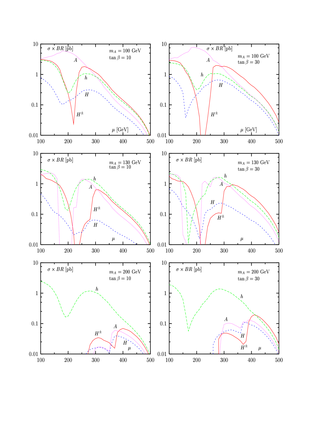
Figure 1: Cross sections times branching ratios for Higgs production in Sc1.

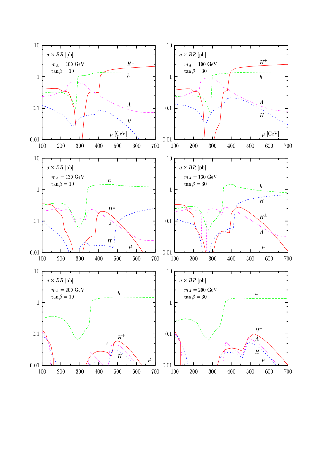
Figure 2: Cross sections times branching ratios for Higgs production in Sc2.

Figure 3: Cross sections times branching ratios for Higgs production in Sc3.

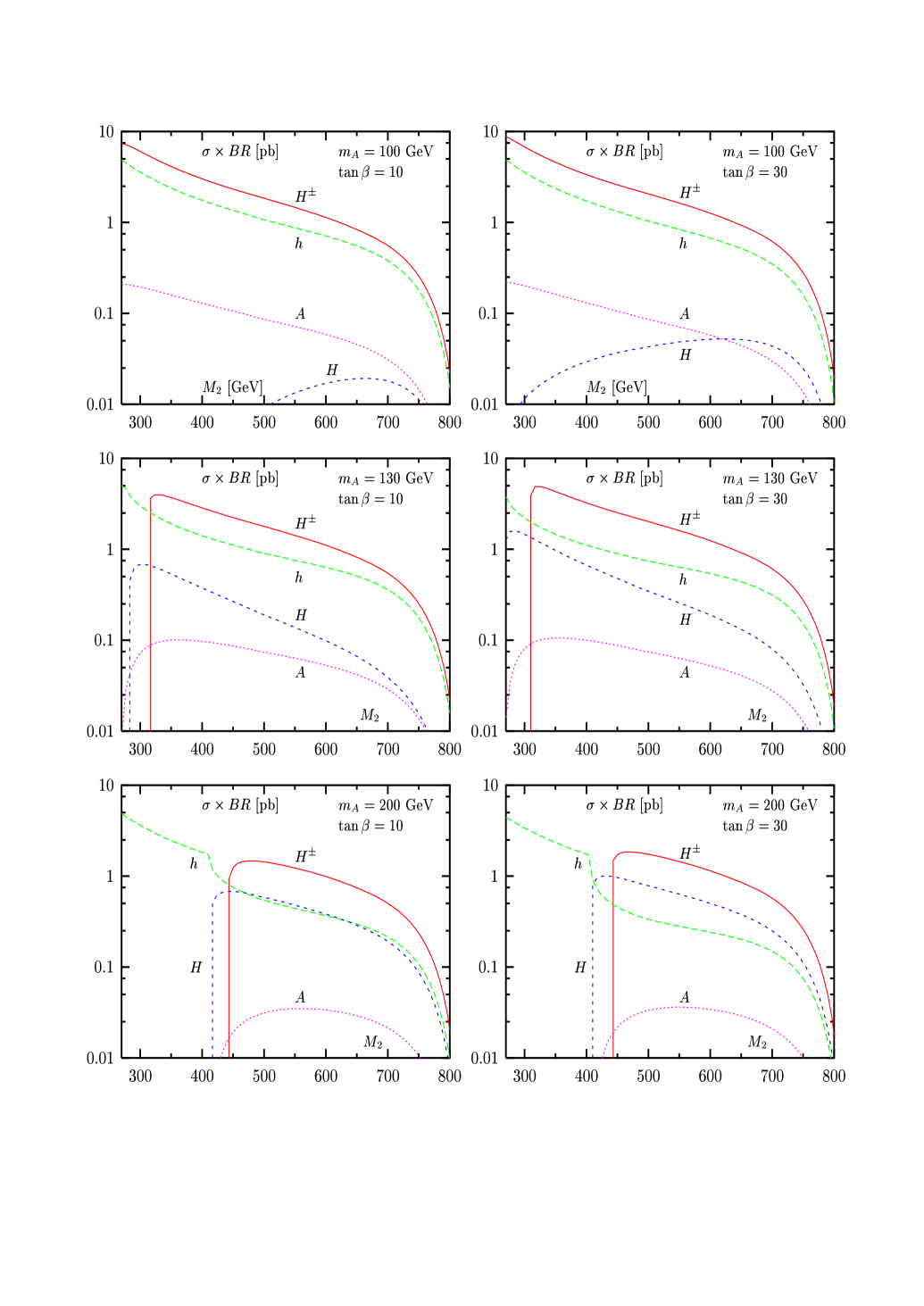
Figure 4: Cross sections times branching ratios for Higgs production in Sc4.

Finally, in Fig. 5, we show the cross sections times branching ratios in the four selected scenarios in the case $M_{A}=150$ GeV and $\tan\beta=5$. Since, as we discussed earlier, the dependence on the value of $\tan\beta$ is not very pronounced, the trend is half–way between what occurs for $M_{A}=130$ GeV and for $M_{A}=200$ GeV. Except for the regions of intermediate $\mu$ value in Sc1 and Sc2 and small $M_{2}$ values in Sc4, $\sigma\times$ BR for the production of the heavier Higgs bosons $H,A$ and $H^{\pm}$ via the cascades are substantial, exceeding the level of 0.1 fb in large regions and even reaching the level of a few picobarns in some cases.

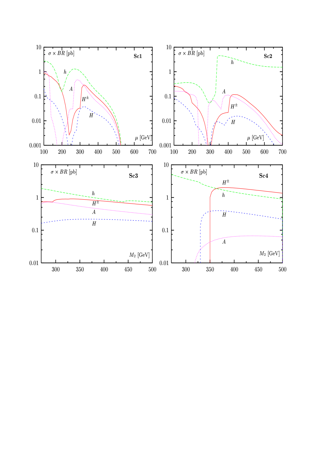
Figure 5: Cross sections times branching ratios for MSSM Higgs boson production for $M_{A}=150$ GeV and $tan\beta=5$ in the four scenarios Sc1 to Sc4.

2.3 Higgs bosons from direct decays of stops and sbottoms

If the mass splitting between two squarks of the same generation is large enough, as is generally the case of the $(\tilde{t},\tilde{b})$ iso–doublet, the heavier squark can decay into a lighter one plus a Higgs boson $\Phi=h,H,A$ [or a $Z$ boson]. If, in addition, there is enough mass splitting between the stops and sbottoms, it is possible for the heavier one to decay into the lighter one and $H^{\pm}$ [or $W^{\pm}$] states. The case of charged Higgs bosons has been studied in detail in Ref. [14] and we concentrate here on the stop and sbottom decays into the neutral Higgs particles, $\tilde{t}_{2}\to\tilde{t}_{1}\Phi$ and $\tilde{b}_{2}\to\tilde{b}_{1}\Phi$.

While the production mechanisms for stops and sbottoms are mainly governed by QCD and the cross sections depend only on the mass of these particles [as well as on the gluino mass when the decays $\tilde{g}\to\tilde{t}t,\tilde{b}b$ are kinematically possible], their subsequent decay rates into Higgs particles depend on many parameters. First, since these squarks are heavy, they have many possible decay modes besides the ones into Higgs bosons discussed here: decays into charginos/neutralinos and quarks, which in general have rather sizable decay widths, as well as decays into gauge bosons. In addition, these decays depend strongly on the Higgs–squark couplings, which in the case of the neutral Higgs particles are given by [see Ref. [14] for a discussion of the couplings and decay widths]:

$$g_{\tilde{q}_{1}\tilde{q}_{2}h} \propto M_{Z}^{2}\sin 2\theta_{q}(2I_{q}^{3}-4e_{q}s_{W}^{2})\sin(\alpha+\beta)+2m_{q}\cos 2\theta_{q}(A_{q}r_{2}^{q}+2I_{q}^{3}\,\mu\,r_{1}^{q})$$

$$g_{\tilde{q}_{1}\tilde{q}_{2}H} \propto -M_{Z}^{2}\sin 2\theta_{q}(2I_{q}^{3}-4e_{q}s_{W}^{2})\cos(\alpha+\beta)+2m_{q}\cos 2\theta_{q}(A_{q}r_{1}^{q}-2I_{q}^{3}\,\mu\,r_{2}^{q})$$

$$g_{\tilde{q}_{1}\tilde{q}_{2}A} = -g_{\tilde{q}_{2}\tilde{q}_{1}A}\propto m_{q}\bigg{[}\mu+A_{q}(\tan\beta)^{-2I_{q}^{3}}\bigg{]}$$ (5)

where $\alpha$ is the mixing angle in the CP–even Higgs sector of the MSSM, $\theta_{q}$ is the squark mixing angle [for $\theta_{q}=0$, $\tilde{q}_{1}=\tilde{q}_{R}$ in general], and the coefficients $r^{q}_{1,2}$ are the normalization factors of the $h,H$ boson couplings to fermions normalised to the SM Higgs boson coupling. The largest component of the CP–even Higgs boson couplings is the one proportional to the quark mass [in the case of sbottom couplings, a $\tan\beta$ enhancement is present for the coupling of the $H$ state]. However, if the mass splitting between the two squarks is large, the squark mixing angle approaches the value $|\theta_{q}|\sim\pi/4$ and the term $\cos 2\theta_{q}$ approaches zero [the other component of the coupling, the one proportional to $M_{Z}$, although maximal since $\sin 2\theta_{q}\sim 1$, is not large enough to make the Higgs–squark coupling strong]. In the case of no mixing, where the coupling becomes strong, there is in general not large enough mass splitting between the two squarks [at least if one assumes common scalar mass terms] to make the decays into Higgs bosons possible. Thus, the only decays that could have sizeable partial widths would be the channels $\tilde{t}_{2}(\tilde{b}_{2})\to\tilde{t_{1}}(\tilde{b}_{1})A$ whereas, in the case of sbottoms, a large value of $\tan\beta$ is needed to make the sbottom mass splitting large for the decay to occur and to compensate for the smallness of $m_{b}$ in the coupling to have a sizeable rate.

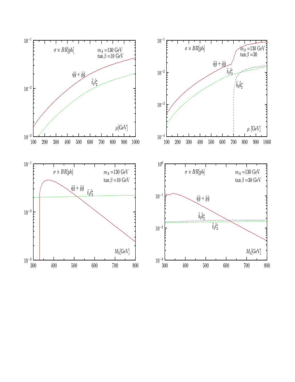
Figure 6: Cross sections times branching ratios for the production of the pseudoscalar Higgs boson from direct decays of heavier stop and sbottom squarks, $\tilde{t}_{2}(\tilde{b}_{2})\to A+\tilde{t}_{1}(\tilde{b}_{1})$, for the values $M_{A}=130$ GeV and $tan\beta=10$ (left panel) and 30 (right panel). The full lines correspond to $\tilde{t}_{2},\tilde{b}_{2}$ squarks originating from decays of gluinos produced in $pp\to\tilde{q}\tilde{g}$ and $\tilde{g}\tilde{g}$ processes, while the dashed lines correspond to top and bottom squarks produced directly in the processes $pp\to\tilde{t}_{2}\tilde{t}_{2}^{*},\tilde{b}_{2}\tilde{b}_{2}^{*}$.

In Fig. 6, we present the cross sections times branching ratios for the production of a single $A$ boson in these cascade decays. We have taken into account all production channels for gluinos and squarks, including the third generation and all possible decays of squarks, i.e. decays into $\chi$ states and quarks, decays into gauge bosons and the possible decays into $H^{\pm}$ bosons. Representative values of the parameters are: $m_{\tilde{q}}=600$ GeV assuming all soft squark masses are degenerate, $m_{\tilde{g}}=3M_{2}$, $A_{q}=1.5$ TeV and $\tan\beta=10,30$; we fixed the pseudoscalar Higgs mass to $M_{A}=130$ GeV and varied $M_{2}$ or $\mu$.

The upper figures show $\sigma\times$BR as a function of $\mu$ for the fixed value $M_{2}=400$ GeV. The solid lines represent the contribution from $\tilde{g}$ cascade decays with the production processes $\tilde{g}\tilde{g}$ and $\tilde{q}\tilde{g}$, whereas the dashed lines are for direct production of $\tilde{q}_{2}\tilde{q}_{2}^{\ast}$ pairs [note that for $\tan\beta=10$, the sbottom contribution is absent as the mass splitting between $\tilde{b}_{2}$ and $\tilde{b}_{1}$ is not sufficient to access the decay $\tilde{b}_{2}\rightarrow\tilde{b}_{1}+A$]. The rates increase with increasing $\mu$ values for two reasons: first, the decay rates $\tilde{t}_{2}\rightarrow\tilde{t}_{1}+A$ increase with $\mu$, as can be seen from the $A\tilde{t}_{1}\tilde{t}_{2}$ coupling discussed above; secondly, a smaller phase space is accessible to stop decays into the heavier charginos and neutralinos, at higher values of $\mu$. [Note that the production cross sections are not sensitive to $\mu$, except for a mild dependence of the $\tilde{t}_{2}$ mass on this parameter.] For the higher $\tan\beta$ case, the situation is similar, except that at a certain value of $\mu~{}(\sim 700$ GeV), the splitting between $m_{\tilde{b}_{2}}$ and $m_{\tilde{b}_{1}}$ becomes large enough to permit the opening of the channel $\tilde{b}_{2}\rightarrow\tilde{b}_{1}+A$, which eventually contributes in both the $\tilde{g}$ cascade decay and in the direct production of $\tilde{b}_{2}$.

The two lower figures show $\sigma\times$BR as functions of $M_{2}$ with a fixed value of $\mu=1000$ GeV. In the low $\tan\beta$ case, the decay of $\tilde{b}_{2}\to\tilde{b}_{1}A$ is not accessible [as we have seen earlier], whereas for the high $\tan\beta$ case it contributes at the same level as $\tilde{t}_{2}$. Here, the rate out of the $\tilde{g}$ cascade decay falls very sharply as the gluino production cross sections decrease with increasing $M_{2}=\frac{1}{3}m_{\tilde{g}}$. On the other hand, the stop and sbottom production cross sections are almost independent of $M_{2}$; their slightly rising behaviour is due to the increased decay branching ratios in the $A$ boson because of the suppressed rates in the gaugino decay channels, which are more phase–space–disfavoured for larger $M_{2}$.

Thus, the production of $A$ bosons from direct decays of $\tilde{t},\tilde{b}$ squarks [as well as the production of $H^{\pm}$ bosons from the decays $\tilde{b}\to\tilde{t}_{1}H^{-}$, which were discussed in Ref. [14] and found to lead to similar results], although in general with much smaller cross sections times branching ratios than Higgs production from cascades involving charginos and neutralinos, might lead to the detection of these particles in favourable situations. An interesting feature is that these processes could allow, in principle, to disentangle the $H$ and $A$ bosons in the decoupling limit, which is otherwise very difficult to achieve in other processes.

2.4 Charged Higgs bosons from top decays under SUSY cascade

The decays of the top quarks that are pair–produced at the LHC are known to be a very important source of charged Higgs bosons for $m_{t}>m_{H^{\pm}}$. Situations permitting, as we will see in this section, cascades of SUSY particles leading to top quarks followed by $t\to bH^{\pm}$ may also become a significant source of $H^{\pm}$ bosons.

Charged Higgs bosons can be produced in SUSY cascade decays via the pair production of gluinos, top and bottom squarks, as in eq. (4), followed by their cascades to top quarks, which subsequently decay to charged Higgs bosons. To have a broad estimate of how significant this new source of charged Higgs particles can be, we discuss cases with the four reference scenarios Sc1–Sc4 presented previously, and calculate the rates for the production of a single charged Higgs boson final state from these cascades. To simplify our discussion, we will not consider the possibility of $H^{\pm}$ production via the $\tilde{b}\tilde{g}$ production mechanism [which has a very low cross section] as well as from decays of heavier chargino and neutralino states, $\chi\rightarrow t+X$ [which would simply increase the sample].

In Fig. 7, we present the results of our study for the four scenarios with the choice $\tan\beta=30$ and $M_{H^{\pm}}=130$ GeV, in terms of variations of cross sections for different production processes, times the branching ratios for the decays $\tilde{g},\tilde{q}\to t+X$ and $t\to bH^{\pm}$. The variations are presented with respect to $\mu$ for Sc1 and Sc2 and with respect to $M_{2}$ for Sc3 and Sc4. We do not present the results for a lower $\tan\beta$ value since it can be estimated in a straightforward manner from the one we are analysing: while the production cross sections and decay branching ratios of SUSY particles remain almost constant, the final $\sigma\times$BR drops by a factor $\sim 1/\tan^{2}\beta$ [i.e. by a factor $\sim 9$ when going from $\tan\beta=30$ to 10] because of the suppressed Yukawa coupling, $g_{H^{\pm}tb}\propto m_{b}\tan\beta$ [the component of this coupling that is proportional to $m_{t}$ is suppressed by a factor $1/\tan\beta$]. Therefore, the total $\sigma\times$BR in the $\tan\beta=10$ case is one order of magnitude smaller than in Fig. 7, while the relative magnitude of the various contributions is approximately the same. Note that, in each figure, the long arrow along the $y$ axis represents the $H^{\pm}$ production cross section via direct $t\bar{t}$ production.

The $\sigma\times$BRs are suppressed by roughly an order of magnitude when going from Sc1 to Sc2 owing to an increased gluino mass and consequently larger squark masses. The variations with respect to $\mu$ present in these scenarios are mainly determined by the resulting variation of the $\tilde{t}t\chi_{i}^{0}$ and $\tilde{b}t\chi_{i}^{\pm}$ couplings. For small $\mu$ values [$\ll M_{2}$] the lighter neutralinos and chargino have masses $m_{\chi_{1,2}^{0}},m_{\chi_{1}^{\pm}}\simeq\mu$ while they are higgsino–like, yielding larger branching ratios in those $\tilde{g}$ decay channels and also for $\tilde{t}_{1}\to t\chi_{j}^{0}$($j=$1–4). However, at a certain value of $\mu$, $\chi_{3}^{0},\chi_{4}^{0}$ become so heavy that they are not accessible in stop decay; this results in a smaller or vanishing BR($\tilde{t}_{1}\rightarrow t\chi^{0}_{3,4}$) value. A further increment of $\sigma\times$BR beyond this $\mu$ value in Sc1 is due to a gradual increment of the gaugino content of $\chi_{1,2}^{0}$.

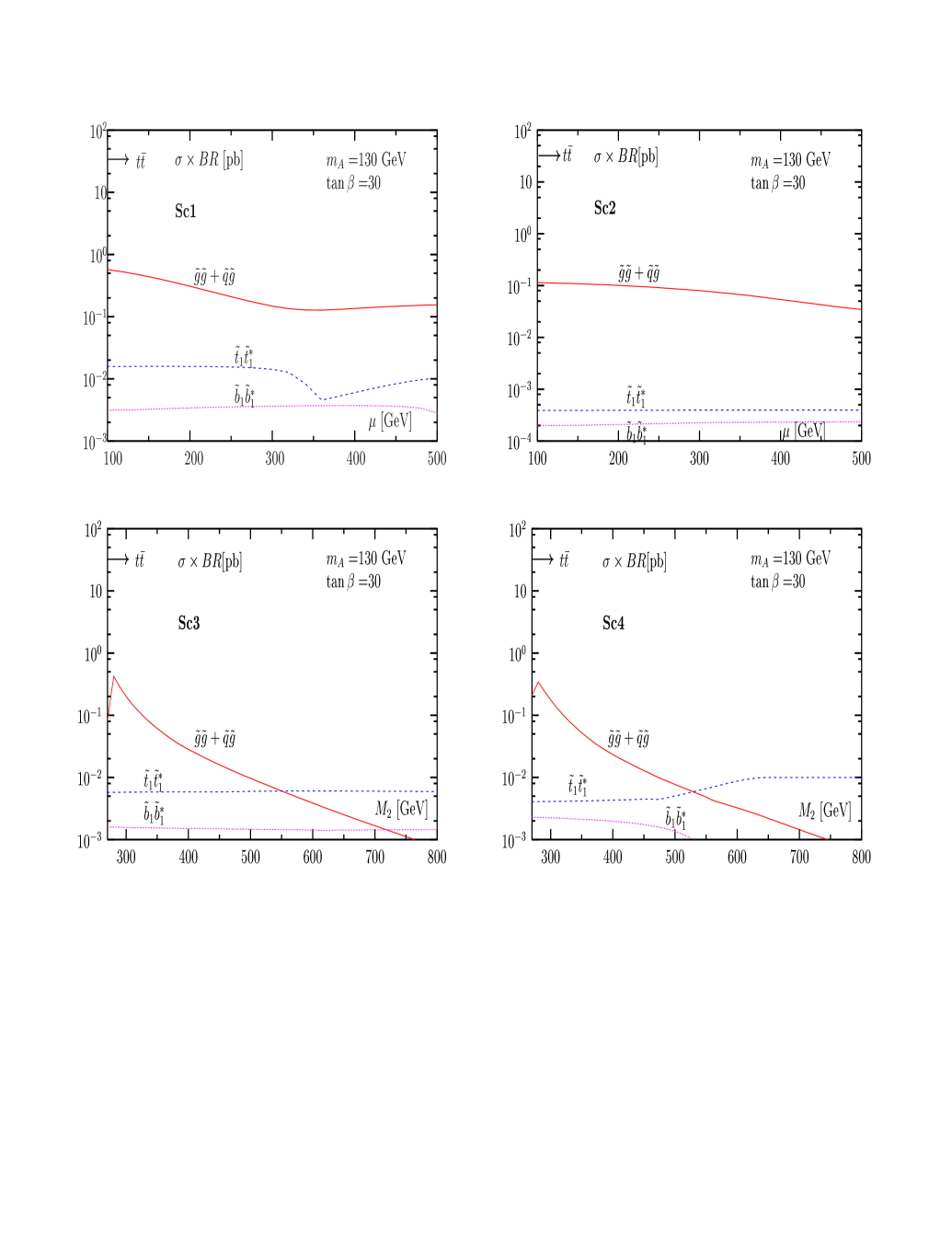
Figure 7: Cross sections times branching ratios for charged Higgs boson production from decays of top quarks originating from cascade decays of strongly interacting SUSY particles in the scenarios Sc1 to Sc4 and for the values $M_{A}=130$ GeV and $tan\beta=30$. For $tan\beta=10$, the trend is similar except that the rates are one order of magnitude smaller. The arrows on top of the figures correspond to the cross section for $gg/q\bar{q}\to t\bar{t}$ times the branching ratio for the decays $t\to H^{+}b$ and $\bar{t}\to H^{-}\bar{b}$.

The profile of the $\tilde{g}$ contribution in Sc1 roughly follows that of $\tilde{t}_{1}\tilde{t}_{1}^{*}$, because the same decay mode $\tilde{t}_{1}\to t\chi_{1}^{0}$ is involved there, to end up with top quarks. The flatness of $\sigma\times$BR for $\tilde{b}_{1}\tilde{b}_{1}^{*}$ production then indicates the low sensitivity of the $\tilde{b}\chi^{\pm}t$ coupling to $\mu$, which is due to the small $m_{b}$ value. For Sc2 the trend is similar, except for the fact that now, the kinks do not appear in the frame. This is due to an increased value of $m_{\tilde{g}}$ [and hence, of $m_{\tilde{q}}=1.2m_{\tilde{g}}$] which effectively pushes $m_{\tilde{t}_{1}}$ to higher values, enabling access to all neutralino states in its decay $\tilde{t}_{1}\rightarrow t\chi_{j}^{0}$ for the entire range of $\mu$.

In Sc3 and Sc4 the contributions from $\tilde{g}\tilde{g}$ and $\tilde{g}\tilde{q}$ production drop naturally with increasing $M_{2}=\frac{1}{3}M_{\tilde{g}}$, as a result of the smaller production cross section for heavier gluinos. The peaks at about $M_{2}\simeq 270$ GeV indicate the onset of the two–body decay of a gluino, $\tilde{g}\rightarrow t\tilde{t}_{1}$. While going from Sc3 to Sc4, we see that the situation does not change much, except for a slight increase of $\sigma\times$BR in the $\tilde{t}_{1}$ pair–production case and a drop in the $\tilde{b}_{1}$ pair–production case beyond 500 GeV in Sc4. The flatness of the $\tilde{t}_{1}\tilde{t}_{1}^{*}$ contributions in Sc3 indicates that the main contribution is coming from $\tilde{t}_{1}\to t\chi_{i}^{0}$ where $i=$1 and 2, i.e. from the lighter neutralinos with masses close to $\mu$. In the case of sbottoms, the main decay mode seems also to be $\tilde{b}_{1}\to t\chi_{1}^{-}$, this chargino being a higgsino.

With $\mu=1$ TeV for Sc4, the decay $\tilde{b}_{1}\to t\chi_{1}^{-}$ gradually drops with increasing $M_{2}$, leading to a decrease of available phase–space [here, the lighter chargino is gaugino–like] and gets closed completely for a high $M_{2}$ value. However, in the stop case there is an increase in $\sigma\times$BR at about 500 GeV for these contributions, which indicates the onset of a gradual increment of the branching ratio $\tilde{t}_{1}\rightarrow t\chi_{1}^{0}$, at the expense of other channels including decays into higher neutralinos and charginos as they are getting closer to phase–space suppression with the increase of $M_{2}$ for a value of $\mu$ as high as 1 TeV.

Thus, for the large value of $\tan\beta=30$ considered and for Sc1 and Sc2, this additional contribution to single charged Higgs production may even become comparable to the one from the cascades involving charginos and neutralinos, in a rather conservative estimate [the cross sections times branching ratios being at the level of 0.1 pb]. For Sc3 and Sc4, these new contributions can only be significant for low gluino masses and naturally drop sharply with the increase in the latter. As mentioned already, and contrary to the processes discussed in section 2.2, the event rates decrease quadratically with $\tan\beta$ and, for instance, are an order of magnitude smaller for $\tan\beta=10$.

In short, for not too heavy a gluino, $m_{\tilde{g}}\raisebox{-3.69899pt}{~{}\shortstack{$<$ \\ [-0.07cm] $\sim$}}~{}1$ TeV, and large values of $\tan\beta$, $\tan\beta\raisebox{-3.69899pt}{~{}\shortstack{$>$ \\ [-0.07cm] $\sim$}}~{}20$, top quarks coming from SUSY particle cascade decays may contribute heavily to charged Higgs boson final states in some regions of the MSSM parameter space. This would always strengthen the signal, although one has to be rather meticulous about the backgrounds [in particular, it would not be an easy task to separate these events from the ones where the $H^{\pm}$ bosons originate from the top quarks, which are directly produced].

3. Detector simulation analysis

In the previous section, the production mechanism of MSSM Higgs bosons through strongly interacting SUSY particle cascade decays has been extensively discussed for several SUSY scenarios. The important feature of this mechanism is the quasi–independence of the production cross sections times branching ratios on the value of $\tan\beta$. This is in contrast to the strong $\tan\beta$ dependence of the direct production mechanisms for the heavier charged and neutral MSSM Higgs bosons, which in the standard processes [$gg\to H/A$ or $gg/q\bar{q}\to b\bar{b}H/A$ for the neutral Higgs bosons and $gg\to t\bar{b}H^{-}$ or $gb\to H^{-}t$ for the charged Higgs particles] lead to a significant number of events only for larger value of this parameter, for which the $Hb\bar{b},Ab\bar{b}$ and $H^{\pm}tb$ couplings are sufficiently enhanced. On the other hand, the masses of the MSSM Higgs bosons accessible in the SUSY cascade decays will probably be limited to the range $M_{A}\raisebox{-3.69899pt}{~{}\shortstack{$<$ \\ [-0.07cm] $\sim$}}~{}250$ GeV by phase–space considerations. Therefore, one might hope to cover the lacuna in the discovery reach for the heavy MSSM Higgs bosons at the LHC, which is left after including the SM [and possibly sparticle] decay modes of these particles, i.e. for low pseudoscalar Higgs boson masses, 120 GeV $\raisebox{-3.69899pt}{~{}\shortstack{$<$ \\ [-0.07cm] $\sim$}}~{}M_{A}\raisebox{-3.69899pt}{~{}\shortstack{$<$ \\ [-0.07cm] $\sim$}}~{}$ 200 GeV and moderately small $\tan\beta$ values, $3\raisebox{-3.69899pt}{~{}\shortstack{$<$ \\ [-0.07cm] $\sim$}}~{}\tan\beta\raisebox{-3.69899pt}{~{}\shortstack{$<$ \\ [-0.07cm] $\sim$}}~{}10$.

In this section, we will present a first analysis that will demonstrate the detection potential of the MSSM Higgs bosons in SUSY particle cascade decays. As already mentioned, the subject is rather involved and in the present paper, we will simply perform a fast Monte–Carlo simulation of the production signal and the various SM and SUSY backgrounds for $H,A$ and $H^{\pm}$ boson production via squark and gluino decays through the big and small cascades. [We will not discuss direct decays of top and bottom squarks into Higgs particles or the production of $H^{\pm}$ bosons through top quark decays]. For illustration, we will focus on the case of $\tan\beta=5$ and $M_{A}=150$ GeV, which leads to a light Higgs boson with a mass of $M_{h}\simeq 110$ GeV [since $h$ is not yet SM–like for this set of parameters, this mass value is not yet excluded by LEP2 searches] and a charged Higgs boson with a mass $M_{H^{\pm}}\simeq 170$ GeV [a value for which the decays $t\to H^{+}b$ would be strongly suppressed], in the scenarios discussed in section 2. The cross sections times branching ratios for these scenarios have been displayed in Fig. 5.

The signal and the background events are generated with HERWIG 6.4 [26]. The SUSY spectrum is calculated with ISASUSY 7.58 [27] and then interfaced to HERWIG using the ISAWIG package [28]. To be as realistic as possible, we also simulate some aspects of the CMS detector using CMSJET 4.801 [23], which contains a parametrized description of the CMS detector response. The effects of event pile–up at the LHC have not been included, but are expected to be small for our analysis. The features that will allow the distinction between the Higgs boson signals from the SM and SUSY backgrounds will be discussed in the next two subsections, and we will argue that the SM backgrounds can be efficiently suppressed. However, a more difficult task will be to distinguish the signals from other SUSY cascade decay processes since all squark and gluino production at the LHC will end up in lightest neutralinos and fermions through gaugino and slepton decays. Hence, a good understanding of the nature of these SUSY backgrounds will be needed prior to any search for MSSM Higgs bosons in cascade decays.

3.1 Neutral Higgs bosons

We start by describing a first–analysis strategy that will allow the observation of the neutral $h,H$ and $A$ bosons produced in the squark/gluino cascades. Two decay modes of these neutral Higgs particles are promising, namely $A,H\rightarrow b\bar{b}$, with a branching ratio around 90%, and $A,H\rightarrow\tau\tau$, with a branching ratio around 10% [the branching ratios are slightly smaller in the case of the lighter $h$ boson]. Because of the dominant branching rate, we will now focus on the $b\bar{b}$ decays, although the $\tau^{+}\tau^{-}$ decay may have some advantages due to the lower multiplicity of $\tau$–jets with respect to $b$–jets in the cascade background. Eventually both modes should be studied since the ratio of their signals could be used to support the evidence for a Higgs signal in the SUSY cascade decays.

In all scenarios, the $h,H$ and $A$ bosons originate from the $\tilde{g}\tilde{g}$, $\tilde{q}\tilde{q}$, $\tilde{q}\tilde{q}^{*}$ or $\tilde{q}\tilde{g}$ production processes through the chain illustrated in eq. (1) or (2). In Sc1 and Sc3, only the first chain is allowed, i.e. only the “big cascade” mechanisms are at work. In Sc2, the light $h$ boson can be produced through the “little cascade” mechanism of eq. (2). In Sc4, also the $H,A$ bosons can be produced in the little cascades. In all cases the background consists of the same $\tilde{g}\tilde{g}$, $\tilde{q}\tilde{q}$, $\tilde{q}\tilde{q}^{*},\tilde{q}\tilde{g}$ processes, where the squarks and gluinos decay into neutralinos and charginos that do not lead to Higgs bosons in their subsequent decay chains.

We will study the features of the signal and the backgrounds in order to determine a set of selection criteria that should serve the following generic purposes:

• They should make sure that the events can pass the CMS on-line trigger levels with a high efficiency.

• They should reduce the SM backgrounds to the level where they are negligible with respect to the SUSY backgrounds.

These two purposes are closely related, since the triggers are designed to reject SM jet backgrounds. In contrast to SM processes, cascade decay Higgs events contain a large number of very energetic jets and a large transverse missing energy. By selecting only events with these features using the criteria that we will propose, trigger efficiencies of more than 90% can be reached [24]. Additional cuts intending to suppress the SUSY background i.e. the SUSY events not containing any Higgs bosons, will depend on the details of the kinematics of this background. In the present paper, to be as unbiased as possible, we will not adapt any special cuts to reject this SUSY background. After suppression of the SM background, we will merely look for resonances in the bb invariant mass spectrum for the four scenarios, comparing this spectrum to its equivalent in the case where Higgs boson production in the SUSY cascades is not allowed.

We will now discuss the kinematical distributions of the SUSY cascades and the SM background in order to obtain a recipe that allows us to suppress the latter while preserving the former. With ’SUSY cascades’ we mean the production of all sparticles according to cross sections obtained from the four scenarios as described in the previous section.

The concrete parameter choices for these scenarios are [the gluino mass $m_{\tilde{g}}$ has been slightly changed in Sc3 and Sc4 to obtain a spectrum that is closer to the one discussed in section 2, while the common slepton mass has been fixed in all four scenarios to the value $m_{\tilde{l}}$ = 500 GeV]:

• Sc1: $M_{2}=2M_{1}=200$ GeV, $\mu=300$ GeV, $m_{\tilde{g}}=600$ GeV and $m_{\tilde{q}}=720$ GeV.

• Sc2: $M_{2}=2M_{1}=300$ GeV, $\mu=450$ GeV, $m_{\tilde{g}}=900$ GeV and $m_{\tilde{q}}=1080$ GeV.

• Sc3: $M_{2}=2M_{1}=350$ GeV, $\mu=150$ GeV, $m_{\tilde{g}}=1200$ GeV and $m_{\tilde{q}}=800$ GeV.

• Sc4: $M_{2}=2M_{1}=350$ GeV, $\mu=1000$ GeV, $m_{\tilde{g}}=1200$ GeV and $m_{\tilde{q}}=800$ GeV.

As SM backgrounds, we have only simulated the main $t\bar{t}$ process. Also other QCD processes [$b\bar{b}$, $c\bar{c}$ and light quark production] will contribute to the SM background; however, it is very difficult to produce a reliable QCD sample in this case, since extreme kinematical fluctuations are necessary for this type of background to be within the signal cuts. Therefore we have not included the QCD background, being confident that any set of criteria that is able to suppress the $t\bar{t}$ background will also be effective against the other QCD background. We recall that ISASUSY 7.58 and HERWIG 6.4 are used for the event generation and that the detector aspects were simulated using CMSJET 4.801 [23], which contains fast parametrizations of the CMS detector response and a parametrized track reconstruction performance based on GEANT simulations for $b$–quark tagging [25]. Results for signal and background are summarized in Figs. 8–11.

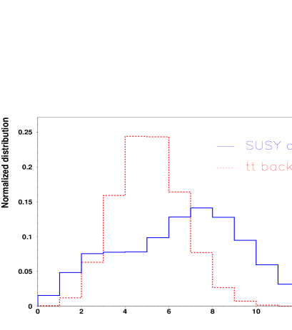
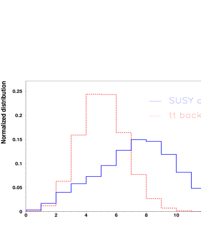
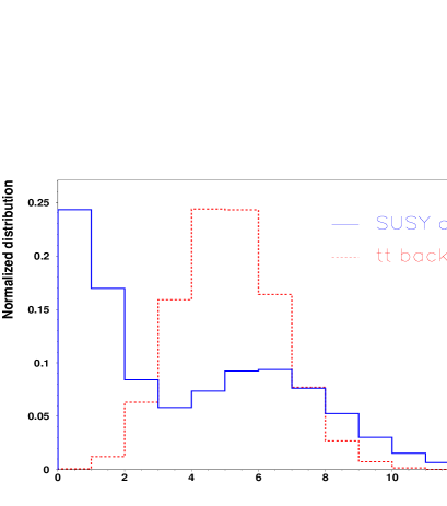
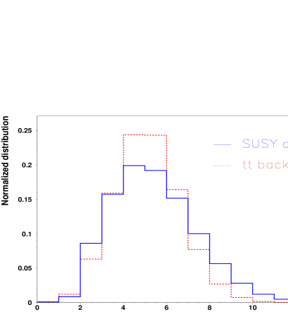
Figure 8: Normalized distribution of the jet multiplicity in the SUSY cascades (full line) and the SM $t\bar{t}$ background (dashed line) events, for the four scenarios. Typically, the SUSY cascades events contain more jets than the SM background events.

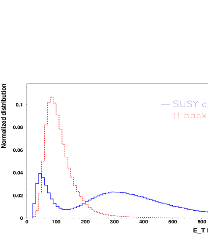
Figure 9: Normalized distribution of the $E_{T}$ of the hardest jet in the SUSY cascades (full line) and the SM $t\bar{t}$ background (dashed line) events, for the four scenarios. The distributions peak around 100 GeV for the SM background and above 300 GeV for the SUSY cascades.

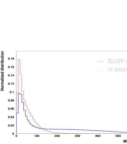
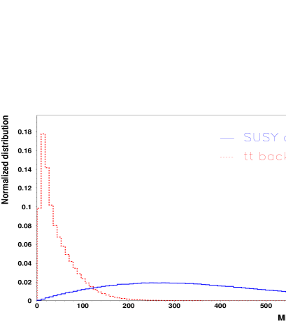
Figure 10: Normalized distribution of the transverse missing energy in the SUSY cascades (full line) and the SM $t\bar{t}$ background (dashed line) events, for the four scenarios. The distribution of the SM background peaks at low values and drops steeply, while the SUSY cascades has a very broad distribution reaching very high values.

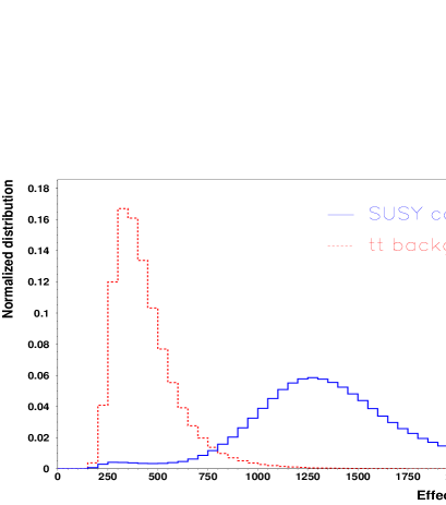
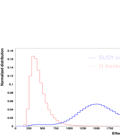
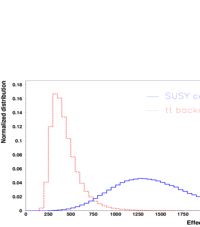
Figure 11: Normalized distribution of the effective mass consisting of the sum of the $E_{T}$ of the jets and the $E_{T}^{\rm miss}$ in the SUSY cascades (full line) and the SM $t\bar{t}$ background (dashed line) events, for the four scenarios. The distributions of the signal and the SM background are clearly separated in all scenarios.

In Fig. 8 the jet multiplicity is shown, for the SUSY cascades and the SM $t\bar{t}$ background, for each of the four scenarios. The first two scenarios have a jet multiplicity distribution that peaks around 8 jets, while the two last scenarios show somewhat lower jet multiplicities. This is linked to the hierarchy of squark, gluino and gaugino masses as described in section 2. For the SM $t\bar{t}$ background, the distribution peaks around 5 jets. Requiring a large number of jets in the event will enhance the sparticle production versus the SM background in most scenarios.

In Fig. 9, we can see the transverse energy of the hardest jet in the event, for the SUSY cascades and the SM $t\bar{t}$ background events, in each of the four scenarios. The distribution peaks around 100 GeV for the SM background and above 300 GeV for the SUSY cascades. Demanding the $E_{T}$ of the hardest jet to be above $\sim$ 300 GeV will therefore strongly suppress the SM background.

Fig. 10 shows the transverse missing energy in the events, for the SUSY cascades and the SM $t\bar{t}$ background, in each of the four scenarios. The distribution of the SM background peaks at low values and drops steeply, while the SUSY cascades have a very broad distribution reaching very high values. Again, requiring a large $E_{T}^{\rm miss}$ in the events will strongly favor the sparticle production with respect to the SM background.

In Fig. 11, the variable $E_{T}^{\rm total}$ is shown, consisting of the sum of the $E_{T}$ of all the jets and the $E_{T}^{\rm miss}$ in the event. The distributions of the SM $t\bar{t}$ background and the SUSY cascades are clearly separated in each of the four scenarios. Selecting only events in which $E_{T}^{\rm total}$ is above $\sim$ 1200 GeV will help suppress the SM background. This selection cut in itself is very effective, however it becomes somewhat redundant if applied after the two previous cuts on $E_{T}^{\rm jet}$ and $E_{T}^{\rm miss}$.

Combining the above observations allow us to strongly suppress the Standard Model background while preserving most of the SUSY cascade events. As a next step, we will study the $b\bar{b}$ invariant mass spectrum and look for resonances of the $h$ (110 GeV), $A$ (150 GeV) and $H$ (160 GeV) Higgs bosons. In order to perform this, we will demand that there be at least two jets in the event carrying a significant $b$–tag and having $E_{T}$ values compatible with the ones originating from a Higgs boson. As mentioned before, no other cut will be made to suppress the SUSY background in view of the uncertain nature of this background. We can thus summarize the selection strategy as follows:

• We require the event to contain at least 5 jets.

• The hardest jet in the event should have an energy $E_{T}$ larger than 300 GeV.

• The transverse missing energy $E_{T}^{\rm miss}$ should be larger than 150 GeV.

• The variable $E_{T}^{total}=\sum E_{T}^{\rm jets}+E_{T}^{\rm miss}$ should have a value larger than 1200 GeV.

• The event should contain at least two $b$–jets with 45 $<$ $E_{T}$ $<$ 120 GeV. In order for the jets to be $b$–tagged, we demand that both jets contain at least two tracks with a significance of the transverse impact parameter $\sigma(ip)=ip_{xy}/\Delta ip_{xy}>$ 3.

If more than two jets in the event fulfill the last condition, the $b\bar{b}$ invariant mass is calculated using the two $b$–jets that are closest to each other in $\eta$–$\phi$ space. Applying the above condition $\sigma(ip)>$ 3 leads to a b–tagging efficiency of about 40%, with a mistagging probability of less than 0.5%.

For each of the four scenarios, we will apply this selection strategy to two different squark/gluino samples: one where all decays are allowed (SUSY signal) and another one where the chargino/neutralino decays into Higgs bosons are switched off (SUSY background). By overlapping the $b\bar{b}$ invariant mass distribution obtained with both samples, we can study the effects of Higgs bosons in the SUSY cascades in an unbiased way. The main results are summarized in Figs. 12–15, assuming a luminosity of $\int{\cal L}=30$ fb^-1.

Fig. 12 shows the $b\bar{b}$ invariant mass spectrum for the SUSY signal overlapped with the SUSY cascade background for Sc1. Both signal and background feature a $Z$ boson peak. In our fast simulation code, the “measured” $M_{b\bar{b}}$ is typically underestimated by about 10% compared to the “true” $M_{b\bar{b}}$. However, the $Z$ peak seems to be shifted to lower values by more that. This is due the large presence of $\chi^{0}_{2}\rightarrow b\bar{b}\chi^{0}_{1}$ decays in the cascades, the $b\bar{b}$ invariant mass distribution of which features a kinematical edge around 80 GeV. This edge interferes with the $Z$ peak and leads to the apparent peak around 70 GeV. There are two more, relatively small, peaks visible in the signal $M_{b\bar{b}}$ spectrum: one around 100 GeV and one around 140 GeV. The first one corresponds to the presence of the $h$ boson while the second one corresponds to the $A,H$ bosons. In this scenario, all Higgs bosons are being produced in the big cascades, i.e. they originate from heavy chargino/neutralino decays. In order to obtain a more convincing S/B ratio, this scenario requires additional selection cuts to suppress the SUSY background. In this figure, also the Standard Model $t\bar{t}$ background is shown. Clearly it is small compared to the SUSY background, justifying our motivation to neglect the QCD background.

Fig. 13 shows the $M_{b\bar{b}}$ distributions for Sc2 and one can see that a large signal peak is coming from $h\rightarrow b\bar{b}$ decays. This is due to the fact that the $h$ boson is being produced in the little cascades [$\chi^{0}_{2}\rightarrow h\chi^{0}_{1}$ has a branching fraction of 96%], while the $H$ and $A$ are only produced in the big cascades. Therefore the $H$, $A$ peak is less visible. Moreover, there is a broad smearing due to the large combinatorial background coming from the wrong pairing of $b$–jets since the $H$ or $A$ state is often accompanied by a $\chi^{0}_{2}$, which decays $\chi^{0}_{2}\rightarrow h\chi^{0}_{1}$, leading to four $b$ quarks in the event. In the background, only the $Z$ boson peak can be seen.

In Fig. 14, the result is shown for the third scenario. There, as can be seen in Fig. 3, the production rates for all Higgs bosons are rather high. There are no little cascades, and the rates for $h$ and $H$, $A$ production are therefore not very different. A double Gaussian fit clearly shows the corresponding peaks, while in the background only the $Z$ boson peak is visible.

In Fig. 15, the $b\bar{b}$ invariant mass spectrum is shown for Sc4. In this case, not only the lighter $h$ boson but also the heavier $H$ and $A$ particles are produced in the little cascades, leading to very clear peaks for the light and the heavy neutral Higgs bosons. Again, in the background spectrum, only the $Z$ boson peak can be observed. Both this scenario and the previous one feature squarks lighter than the gluino [which has a mass around 1 TeV]; from the figures, it is clear that this condition strongly enhances the visibility of the neutral Higgs boson signals.

Conservatively estimating the significance of the peaks as ${\cal{S}}=S/\sqrt{B}$, where $S$ is the number of events in the peak and $B$ the number of events “below” the peak [i.e. below a hand–drawn line between the two shoulders of the peak], we obtain a 5$\sigma$ significance for the $A,H$ peak in Sc4. With 30 fb^-1 of integrated luminosity, enough data are collected to observe a 5$\sigma$ excess also for Sc3. Sc1 and Sc2 will require a more detailed study and/or a larger integrated luminosity.

This simple analysis of the neutral Higgs bosons produced in the SUSY cascades shows that this alternative production mechanism looks very promising. The Standard Model backgrounds can be efficiently suppressed by the selection criteria outlined above. By studying the $b\bar{b}$ invariant mass spectrum, we have shown that for all the considered scenarios the neutral Higgs bosons are visible after a few years of low luminosity running of the LHC collider.

This has been exemplified in the case where $M_{A}=150$ GeV and $\tan\beta=5$. However, as discussed in section 2, the dependence of the signal cross sections times branching ratios on the parameter $\tan\beta$ is rather weak in the cascade decays and we can therefore extrapolate this conclusion to all values of this parameter. For the Higgs mass range that can be probed in these processes, we are limited by two factors:

$(i)$ In the low mass range, $M_{A}\raisebox{-3.69899pt}{~{}\shortstack{$>$ \\ [-0.07cm] $\sim$}}~{}90$ GeV, we get rather close to the $Z$ boson peak and the signal and background overlap; however, the cross section times branching ratios for the signal can be rather large in this phase–space–favoured case and the signal peak can be much larger than the background peak. Moreover, by normalizing the $Z\rightarrow b\bar{b}$ distribution to the $Z\rightarrow ee,\mu\mu$ distribution, any excess can be clearly established.

$(ii)$ For larger $M_{A}$ values, the $A,H$ bosons become too heavy and phase space becomes penalizing [the branching ratios for the decays of heavier chargino/neutralino states into the lighter ones and the $H,A$ bosons become too small]. However, in many scenarios one can still have reasonable Higgs production rates up to pseudoscalar masses of the order of $M_{A}=250$ GeV. Certainly, in Sc1–Sc4 discussed here, one can probe masses up to $M_{A}=200$ GeV, since there still are reasonable event rates, as shown in Figs. 1–4.

Therefore, it appears that the heavier MSSM Higgs bosons originating from cascade decays of squarks and gluinos can be detected at the LHC for any value of $\tan\beta$ and for pseudoscalar Higgs boson masses approximately in the mass range between 100 and 200 GeV [the lightest $h$ boson can be detected in its entire mass range] in a few years of LHC running with a moderate luminosity.

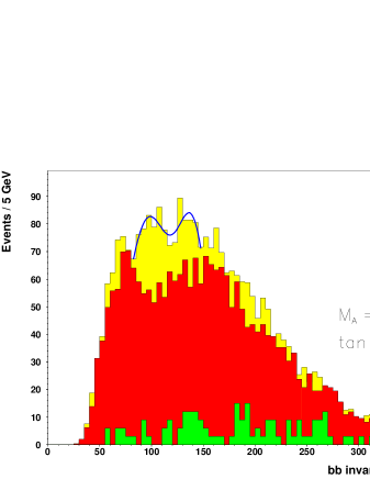
Figure 12: Distribution of the $b\bar{b}$ invariant mass for the SUSY signal events on top of the SUSY cascade background assuming scenario Sc1 (with 30 fb^-1 luminosity). At the bottom, the distribution for the Standard Model $t\bar{t}$ background is plotted. Two rather small peaks can be seen in the signal, corresponding to the presence of $h$ and $A,H$ bosons originating from the big SUSY cascades.

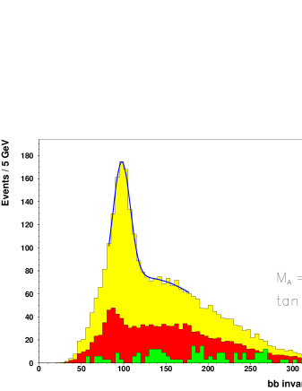
Figure 13: Distribution of the $b\bar{b}$ invariant mass for the SUSY signal events on top of the SUSY cascade background for scenario Sc2 (30 fb^-1). The SM $t\bar{t}$ background is also shown. A large signal peak is visible, corresponding to the $h$ bosons that are abundantly produced in the little cascades; also a much smaller and broader peak can be seen, signaling the presence of $A$ and $H$ bosons coming from the big cascades.

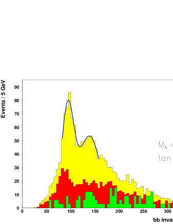
Figure 14: Distribution of the $b\bar{b}$ invariant mass for the SUSY signal events on top of the SUSY cascade background for scenario Sc3 (30 fb^-1). The SM $t\bar{t}$ background is also shown. Two peaks can be distinguished, a large one corresponding to the $h$ boson and a smaller one corresponding to the $A,H$ bosons, all originating from the big cascades.

Figure 15: Distribution of the $b\bar{b}$ invariant mass for the SUSY signal events on top of the SUSY cascade background for scenario Sc4 (30 fb^-1). The SM $t\bar{t}$ background is also shown. Two peaks are clearly visible, corresponding to the $h$ and $A,H$ Higgs bosons, all being produced in the little cascades.

3.2 Charged Higgs bosons

After having demonstrated the potential for observing the neutral Higgs bosons in the SUSY cascade decays, we will now study the charged Higgs production through this mechanism. Since in all considered scenarios, $M_{A}\simeq 150$ GeV, the charged Higgs boson mass is close to the top quark mass, $M_{H^{\pm}}\simeq 170$ GeV, and top quark decays into bottom quarks and $H^{\pm}$ bosons will be strongly suppressed by phase space. For the same reason, the charged Higgs decay mode to $t\bar{b}$ will be suppressed and the $H^{\pm}$ particles will decay into $\tau\nu$ final states with a branching ratio of 95% [some small fraction would also decay into $cs$ final states for low values of $\tan\beta$]. This enforces our choice of the decay mode of investigation to be $H^{\pm}\rightarrow\tau^{\pm}\nu_{\tau}$.

We will select events containing a hard $\tau$–jet plus additional hard jets (often $b$-jets) accompanied by a large amount of missing energy due to the presence of the lightest neutralinos and the neutrinos. Since there are numerous sources of missing energy in the cascade decays, an invariant mass reconstruction of the charged Higgs using the $\tau\nu_{\tau}$ mode is not possible. Also, in the $t\bar{b}$ decay mode, if the branching ratio had been sizeable, a reconstruction of the 4–jet system [2 $b$–jets + 2 jets from the $W$ boson] would have suffered from a huge combinatorial background in the environment of the cascade decays.

Though deprived from the powerful tool of invariant mass reconstruction, the hadronic $H^{\pm}\rightarrow\tau^{\pm}\nu_{\tau}$ mode has a special feature that can be exploited in distinguishing it from the main background decay $W^{\pm}\rightarrow\tau^{\pm}\nu_{\tau}$: the tau polarization effects for both channels are quite different [30].

Indeed, due to the scalar nature of the decaying $H^{+}$ particle, the $\tau^{+}$ lepton from its decay is produced in a left–handed polarization state. In the simplest scenario of $\tau^{+}\rightarrow\pi^{+}\bar{\nu}$ decay, the right–handed $\bar{\nu}$ is preferentially emitted in the direction opposite to the $\tau^{+}$ in the tau rest frame, so as to preserve the polarization. On the contrary, in the background, the $\tau^{+}$ from the $W^{+}\rightarrow\tau^{+}\nu$ decay is produced in a right–handed state due to the vector nature of the $W^{+}$ boson, forcing the $\bar{\nu}$ from $\tau^{+}\rightarrow\pi^{+}\bar{\nu}$ to be emitted in the same direction as the $\tau^{+}$ in the tau rest frame. Therefore, harder pions are expected from the signal than from the $W$ bosons in the background. By selecting events in which the fraction of the $\tau$-jet transverse momentum carried by the charged pion is large, the SM and SUSY background involving $W$ bosons can be suppressed relative to the signal. The tau leptons in the background coming from either $\tilde{\tau}$ and $Z$ decays or the decays of the MSSM neutral Higgs bosons [in particular $H$ and $A$] can however not be suppressed this way.

Thus, as a signature for the charged Higgs boson in the SUSY cascade decays, we will look for highly energetic $\tau$–jets in which the leading charged particle carries most of the momentum.

For the simulations, we have again used ISASUSY 7.58 [27] for the calculation of the SUSY particle spectrum and the HERWIG 6.4 [26] Monte–Carlo event generator for the signal and background generation. This generator takes into account the spin correlations between the production and decay of all heavy fermions, which in our case is important for the top quarks in the $t\bar{t}$ production and SUSY particles in the cascades. To properly account for the tau polarization, the generator was interfaced with the TAUOLA [29] package.

We simulate again the four SUSY scenarios Sc1–Sc4 described in section 2, with production cross sections times branching ratios as given in Fig. 5. For the SM background, again only the $t\bar{t}$ process was considered. Also the $W$ + $n$–jet background will be important, but we have not included it since the standard Monte–Carlo generators do not give a realistic jet transverse energy spectrum for these processes, especially in the high transverse energy region. We are, however, convinced that any selection criterion that is able to suppress the $t\bar{t}$ background, will also successfully reject the $W$ + $n$–jet background. Since the kinematical distributions of the SUSY cascades and the $t\bar{t}$ events are the same as in the neutral Higgs boson case, we can refer to Figs. 8–11 and the related discussion on the selection strategy to suppress the SM background. We will adopt here the same selection criteria.

After eliminating the SM backgrounds, there still remains the more difficult task to discriminate the $H^{\pm}$ bosons from the other particles in the SUSY cascade decays. Tau–leptons in the cascade backgrounds originate mostly from $W$ and $Z$ bosons. Taus coming from these particles will have a somewhat softer spectrum than the ones coming from a 170 GeV charged Higgs boson. Therefore we impose a lower limit on the transverse energy of the $\tau$-jet around the $W$ mass, $E_{T}^{\rm\tau-jet}$ $>$ 80 GeV.

As a measure of the hardness of the charged hadron in the $\tau$–jet, we show in Fig. 16 the distribution of the fraction of the transverse energy $E_{T}^{\rm\tau-jet}$ that is carried by the one-prong charged particle in the jet. The full line corresponds to the SUSY signal [i.e. the cascade decays including the charged Higgs bosons] while the dashed line corresponds to the SUSY backgrounds [i.e. the same cascades where the decays of the heavier charginos/neutralinos to charged Higgs bosons and lighter charginos/neutralinos are forbidden]. Because of the polarization effects as explained above, this distribution peaks at high values for tau leptons coming from scalar charged Higgs bosons, while peaking at low values for tau leptons coming from vector–like $W$ bosons. Requiring that at least 75% of the transverse energy of the $\tau$–jet be carried by the charged hadron, we can enhance the visibility of the signal with respect to the SUSY background.

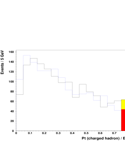
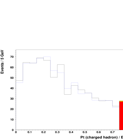
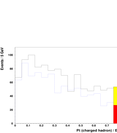
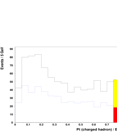
Figure 16: Distribution of the fraction of the $E_{T}^{\rm\tau-jet}$ that is carried by the charged particle in the jet. The full line represents the signal while the dashed line represents the SUSY background. The shaded areas contain the events left after applying the selection cuts, for an integrated luminosity of 30 fb^-1. The charged Higgs signal is clearly visible in Sc3 and Sc4, but not visible in Sc1 and Sc2.

These considerations lead us to the following selection criteria in order to distinguish between signal and background events:

• The events should contain at least five jets.

• The hardest jet in the event should have $E_{T}$ $>$ 300 GeV.

• The transverse missing energy $E_{T}^{\rm miss}$ in the event should be larger than 200 GeV.

• We require exactly one hadronically decaying tau (1-prong), i.e. we demand a narrow jet within $|\eta|\,<\,2.5$, which should contain a hard charged track of $p_{T}\,>\,5$ GeV in a cone of $\Delta R$ = 0.15 rad around the calorimeter jet axis, and it should be isolated, meaning no charged tracks with $p_{T}\,>\,2$ GeV are allowed in a cone of $\Delta R$ = 0.4 rad around the axis.

• The $E_{T}$ of the $\tau$–jet, defined as the $E_{T}$ reconstructed in a cone of $\Delta R$ = 0.4 rad around the jet axis, should be above 80 GeV.

• More than 75% of the $\tau$–jet transverse energy should be carried by the charged track, i.e. we impose the cut $p_{T}^{\pi}/E_{T}^{\rm\tau-jet}$ $>$ 0.75.

Events that satisfy conditions ($i$)–($iii$) can be efficiently triggered on using the jet and missing–energy triggers.

In Fig. 16, the shaded areas represent the number of events left after all selection cuts, for the signal and the SUSY background. The charged Higgs boson signal is clearly visible in Sc3 and Sc4, but not in Sc1 and Sc2. This is because the production cross section for these scenarios are about 10 times smaller than for Sc3 and Sc4, as can be seen from Fig. 5.

Clearly, the evidence for the charged Higgs boson is not as convincing as the invariant mass peaks we obtained in the neutral Higgs boson case. However, in the MSSM, the neutral and charged Higgs boson masses are not independent: since they are are connected through the relation $M^{2}_{H^{\pm}}=M^{2}_{A}+M^{2}_{W}$ [which is valid at leading order but is not strongly affected by radiative corrections], the observation of the neutral Higgs bosons can give definite information on the charged Higgs boson mass. If one then observes an excess in $\tau$–jet events after a selection as illustrated above, one can be rather confident that this excess originates from the production of charged Higgs particles.

4. Conclusion

We have analysed the detection prospects of the neutral and charged Higgs particles of the MSSM in single Higgs final states obtained through the cascade decays of the heavy squarks and gluinos that will be copiously produced at the LHC. We have discussed in detail the case of the production through the cascades involving the heavier charginos and neutralinos [originating from the decays of the strongly interacting SUSY particles] into the lighter charginos and neutralinos and a Higgs boson $\Phi$. This can occur through the “big cascades”, $\chi_{3,4}^{0},\chi_{2}^{\pm}\to\chi_{1,2}^{0},\chi_{1}^{\pm}+\Phi$, as well as through the “small cascades”, $\chi_{2}^{0},\chi_{1}^{\pm}\to\chi_{1}^{0}+\Phi$, or through both cascades, depending on the considered scenario. For illustration, we have selected four scenarios which are expected to cover most of the situations which can occur in the MSSM: squarks either lighter or heavier than gluinos, and light charginos and neutralinos, either of the gaugino– or higgsino–type.

We have shown that in these scenarios and with not too heavy Higgs particles, with masses $M_{\Phi}\raisebox{-3.69899pt}{~{}\shortstack{$<$ \\ [-0.07cm] $\sim$}}~{}200$–250 GeV, the cross sections times branching ratios for the production of at least one neutral or charged MSSM Higgs boson can be substantial at the LHC , resulting in large numbers of signal events with an integrated luminosity of $\int{\cal L}\raisebox{-3.69899pt}{~{}\shortstack{$>$ \\ [-0.07cm] $\sim$}}~{}30$ fb^-1, which is expected to be collected after a few years of running.

We have performed a full Monte–Carlo simulation that takes into account the various signals as well as the SM and SUSY backgrounds and includes a fast simulation of some important aspects of the responce of the CMS detector at the LHC [similar conclusions are expected to be drawn for the ATLAS detector]. We have shown that these final states can indeed be detected in some representative MSSM scenarios. In particular, the heavier CP–even $H$ and the pseudoscalar $A$ bosons can be observed in the region of parameter space $M_{A}\sim 150$ GeV and $\tan\beta\sim 5$, which cannot be probed by searches using the standard Higgs production channels. Therefore, the search for Higgs bosons via the cascade decays could be complementary to the standard searches.

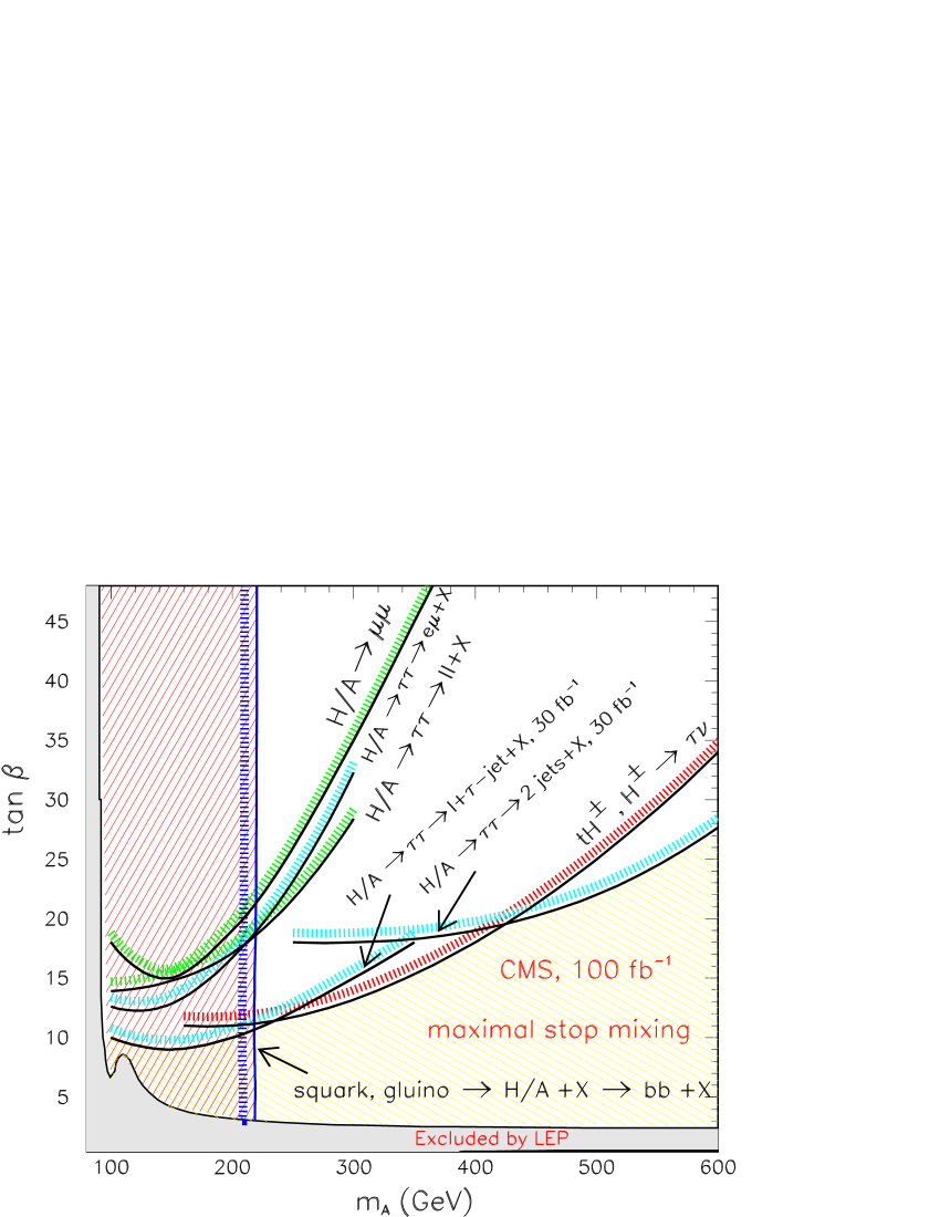
Figure 17: The areas in the $(M_{A},\tan\beta)$ parameter space where the MSSM Higgs bosons can be discovered at CMS with an integrated luminosity of 100 fb^-1. Various detection channels are shown in the case of the standard searches for the maximal stop mixing scenario. The right–hatched and cross–hatched regions show the areas where only the lightest $h$ boson can be observed in these production channels. The left–hatched area is the region where the heavier CP–even $H$ and pseudoscalar $A$ bosons can be observed through the (big) cascade decays of squarks and gluinos in Sc3 with $M_{2}=350$ GeV. A similar contour plot can be obtained in Sc4, where only the little cascade is at work.

This is exemplified in Fig. 17, in which we show the areas of the $(\tan\beta,M_{A}$) parameter space where the MSSM Higgs particles can be detected by the CMS collaboration with an integrated luminosity of $\int{\cal L}\simeq 100$ fb^-1. Besides the usual areas where the Higgs bosons can be probed in SM–like production and decay processes, we exhibit the range of $M_{A}$ values where one can detect, in addition, the $A,H$ and $H^{\pm}$ bosons via the cascade decays in a specific MSSM scenario [namely Sc3, with the value of the parameter $M_{2}$ fixed to $350$ GeV]. The heavier neutral $A,H$ particles can be probed for masses up to $M_{A}\sim 220$ GeV for the entire range of $\tan\beta$ values [as we have shown in our analysis, the cross sections times branching ratios depend only mildly on the value of this parameter], while the charged Higgs particle can be observed for masses up to $M_{H}^{\pm}\sim 200$ GeV [the lighter $h$ boson can of course be detected in the entire ($\tan\beta,M_{A})$ plane in this scenario]. As can be seen, the additional channels can fill some holes of the parameter space where these heavier Higgs particles cannot be observed through the standard processes.

We have also discussed, though only at the level of production cross sections times decay branching fractions, MSSM Higgs boson production through the decays of heavier third–generation squark into the lighter ones, as well as the production of $H^{\pm}$ bosons from the decays of top quarks originating from $\tilde{g},\tilde{q}$ cascade decays. While the rates for Higgs boson production from direct decays of third–generation squarks are in general smaller than in the previous case, they can be substantial for large $\tan\beta$ values in the case where top quarks originating from SUSY cascades decay into $H^{\pm}$ bosons. These additional channels can therefore increase the yield for Higgs particles at the LHC. We did not attempt to perform a Monte–Carlo simulation to verify whether the final states in these channels can indeed be detected in a realistic situation.

The present study does not pretend to be exhaustive. To cover the entire possibilities for MSSM Higgs boson production through SUSY particle cascade decays, many more studies, in particular detailed experimental simulations, are required in order to fully cover this rather complicated subject. Here, we simply made a preliminary investigation in some selected scenarios, which indicates that the detection of Higgs particles in these processes is not at all hopeless and might even complement the searches through the intensively studied SM–like processes in some favourable cases.

We stress again that these cascade processes are important not only because they represent a new source of Higgs bosons, but also because they will be very useful to measure the couplings of supersymmetric particles to Higgs bosons, which would be an essential ingredient to reconstruct the SUSY Lagrangian at low energies and to probe the theory at very high scales.

In addition, if the branching ratios are sufficiently large, the decays of heavy neutralinos into $b\bar{b}$ pairs through Higgs boson intermediate states, $\chi_{3,4}^{0}\rightarrow h,H,A+\chi_{1}^{0}\rightarrow b\bar{b}+\chi_{1}^{0}$, contain information to reconstruct the masses of the heavier neutralinos and could as such help significantly in identifying the supersymmetric particle spectrum at the LHC.

Hence, on their own merit, SUSY particle cascade processes involving Higgs bosons deserve detailed and dedicated studies in the future.

Acknowledgements:

We thank Daniel Denegri, Yann Mambrini and Luc Pape for discussions. A. Datta would like to acknowledge the French MNERT fellowship, the CNRS for partial support and the LPMT for the hospitality accorded to him when this work was initiated; he is supported by a DOE grant DE-FG02–97ER41029. M. Guchait thanks the CERN Theory Division, where part of this work was performed. F. Moortgat is research assistant of the Fund for Scientific Research (FWO-Vlaanderen), Belgium.

References

- [1] For a review on the Higgs sector of the MSSM, see J.F. Gunion, H.E. Haber, G.L. Kane and S. Dawson, “The Higgs Hunter’s Guide”, Addison–Wesley, Reading, 1990.
- [2] For reviews on the MSSM, see: H.P. Nilles, Phys. Rep. 110 (1984) 1; H.E. Haber and G. Kane, Phys. Rep. 117 (1985) 75; R. Barbieri, Riv. Nuov. Cim. 11 (1988) 1; R. Arnowitt and P. Nath, Report CTP-TAMU-52-93; M. Drees and S. Martin hep-ph/9504324; J. Bagger, hep-ph/9604232; A. Djouadi et al., hep-ph/9901246.
- [3] A. Djouadi et al., Proceedings of the Les Houches Workshops in 1999, hep-ph/0002258; D. Cavalli et al., Proceedings of the Les Houches Workshops in 2001, hep-ph/0203056.
- [4] CMS Collaboration, Technical Proposal, CERN/LHCC/94-38 (1994); ATLAS Collaboration, Technical Design Report, CERN/LHCC/99-15 (1999); F. Gianotti, talk given at IECHEP, Budapest, 2001; R. Kinnunen, talk given at SUSY02, Hamburg, 2002.
- [5] The LEP Higgs working group, hep-ex/0107029 and hep-ex/0107030.
- [6] H. Baer et al., Phys. Rev. D36 (1987) 1363; K. Griest and H.E. Haber, Phys. Rev. D37 (1988) 719; J.F. Gunion and H.E. Haber, Nucl. Phys. B307 (1988) 445; A. Djouadi et al., Phys. Lett. B376 (1996) 220, A. Djouadi, J. Kalinowski and P. Zerwas, Z. Phys. C57 (1993) 569 and Z. Phys. C74 (1997) 93; A. Bartl et al., Phys. Lett. B389 (1996) 538; A. Djouadi, Mod. Phys. Lett. A14 (1999) 359; M. Bisset, M. Guchait and S. Moretti, Eur. Phys. J. C19 (2001) 143; F. Moortgat, S. Abdullin and D. Denegri, hep-ph/0112046; F. Moortgat, hep-ph/0105081.
- [7] J.I. Illana et al., Eur. Phys. J.C1 (1998) 149; A. Djouadi, Phys. Lett. B435 (1998) 101; G. Bélanger et al., Nucl. Phys. B581 (2000) 3.
- [8] H. Georgi et al., Phys. Rev. Lett. 40 (1978) 692; A. Djouadi, M. Spira and P.M. Zerwas, Phys. Lett. B264 (1991) 440; S. Dawson, Nucl. Phys. B359 (1991) 283; M. Spira et al., Phys. Lett. B318 (1993) 347 and Nucl. Phys. B453 (1995) 17; S. Dawson, A. Djouadi and M. Spira, Phys. Rev. Lett. 77 (1996) 16; R.V. Harlander and W. Kilgore, Phys. Rev. Lett. 88 (2002) 201801; C. Anastasiou and K. Melnikov, Nucl. Phys. B646 (2002) 220.
- [9] Z. Kunszt, Nucl. Phys. B247 (1984) 339; J. Gunion, Phys. Lett. B253 (1991) 269; J. Dai, J. Gunion and R. Vega, Phys. Lett. B345 (1995) 29; W. Beenakker et al., Phys. Rev. Lett. 87 (2001) 201805; L. Reina and S. Dawson, Phys. Rev. Lett. 87 (2001) 201804.
- [10] A.C. Bawa, C.S. Kim and A.D. Martin, Z. Phys. C47 (1990) 75; V. Barger, R.J.N. Phillips and D.P. Roy, Phys. Lett. B324 (1994) 236; J.F. Gunion, Phys. Lett. B322 (1994) 125; S. Moretti and K. Odagiri, Phys. Rev. D55 (1997) 5627. F. Borzumati, J.-L. Kneur and N. Polonsky, Phys. Rev. D60 (1999) 115011; M. Drees, M. Guchait and D.P. Roy, Phys. Lett. B471 (1999) 39; D. Miller, S. Moretti, D.P. Roy and W. Stirling, Phys. Rev. D61 (2000) 055011.
- [11] A. Arhrib et al., Phys. Rev. D57 (1998) 5860; A. Bartl et al., Phys. Rev. D59 (1999) 115007; A. Djouadi, J.L. Kneur and G. Moultaka, Phys. Rev. Lett. 80 (1998) 1830 and Nucl. Phys. B569 (2000) 53; G. Bélanger, F. Boudjema and K. Sridhar, Nucl. Phys. B568 (2000) 3; A. Dedes and S. Moretti, Eur. Phys. J. C10 (1999) 515 and Phys. Rev. D60 (1999) 015007.
- [12] A. Bartl, W. Majerotto and N. Oshimo, Phys. Lett. B216 (1989) 233. For analyses at the LHC, see for instance: D. Denegri, W. Majerotto and L. Rurua, CMS-NOTE-1997-094, hep–ph/9711357; S. Abdullin et al. (CMS Collaboration), CMS-NOTE-1998-006, J. Phys. G28 (2002) 469; I. Hinchliffe et al., Phys. Rev. D55 (1997) 5520.
- [13] H. Baer, M. Bisset, X. Tata and J. Woodside, Phys. Rev. D46 (1992) 303.
- [14] A. Datta, A. Djouadi, M. Guchait and Y. Mambrini, Phys. Rev. D65 (2002) 015007.
- [15] E. Boos, A. Djouadi, M. Mühlleitner and A. Vologdin, Phys. Rev. D66 (2002) 055004.
- [16] J.F. Gunion and H.E. Haber, Nucl. Phys. B272 (1986) 1; A. Djouadi, J. Kalinowski, P. Ohmann and P.M. Zerwas, hep-ph/9605437.
- [17] A. Djouadi, J. Kalinowski and M. Spira, Comput. Phys. Commun. 108 (1998) 56.
- [18] CTEQ Collaboration (H.L. Lai et al.), Phys. Rev. D55 (1997) 1280.
- [19] W. Beenakker, R. Höpker, M. Spira and P.M. Zerwas, Nucl. Phys. B492 (1997) 51.
- [20] S. Kraml, H. Eberl, A. Bartl, W. Majerotto and W. Porod, Phys. Lett. B386 (1996) 175; A. Djouadi, W. Hollik and C. Junger, Phys. Rev. D55 (1997) 6975; W. Beenakker, R. Hopker, T. Plehn and P.M. Zerwas, Z. Phys. C75 (1997) 349.
- [21] W. Porod, Phys. Rev. D59 (1999) 095009; A. Datta, M. Guchait and K.K. Jeong, Int. J. Mod. Phys. A14 (1999) 2239; A. Djouadi and Y. Mambrini, Phys. Rev. D63 (2001) 115005; C. Boehm, A. Djouadi and Y. Mambrini, Phys. Rev. D61 (2000) 095006.
- [22] A. Bartl, W. Majerotto and W. Porod, Z. Phys. C64, 499 (1994) and (E) C68, 515 (1995); H. Baer et al., Phys. Rev. Lett. 79 (1997) 986 and Phys. Rev. D58 (1998) 075008; A. Djouadi and Y. Mambrini, Phys. Lett. B493 (2000) 120; A. Djouadi, Y. Mambrini and M. Mühlleitner, Eur. Phys. J. C20 (2001) 563.
- [23] S. Abdullin, A. Khanov and N. Stepanov, CMS NOTE-1994/180.
- [24] CMS Collaboration, “The Trigger and DAQ project, Volume 2, The high level trigger, Technical Design Report”, CERN/LHCC 2002-026, CMS TDR 6.2, December 2002.
- [25] The CMS Simulation Package, http://cmsdoc.cern.ch/cmsim/cmsim.html
- [26] G. Corcella et al., “HERWIG 6: An event generator for hadron emission reactions with interfering gluons (including SUSY processes)”, JHEP 0101 (2001) 010.
- [27] H. Baer, F.E. Paige, S.D. Protopopescu and X. Tata, “ISAJET 7.48: A Monte-Carlo event generator for and reactions”, hep-ph/0001086.
- [28] See: http://www.hep.phy.cam.ac.uk/ richardn/HERWIG/ISAWIG/
- [29] S. Jadach, Z. Was and J.H. Kühn, Comput. Phys. Commun. 64 (1991) 275.
- [30] D.P. Roy, Phys. Lett. B459 (1999) 607.