Physics of Electroweak Gauge Bosons

Klaus Mönig

DESY

Platanenalle 6, D-15738 Zeuthen, Germany

E-mail: Klaus.Moenigdesy.de

The study of gauge bosons is interesting in two respects. The properties of gauge bosons are modified by higher order effects that are sensitive to mass scales not directly accessible to experiment. On the other hand interactions amongst gauge bosons are sensitive to the symmetry structure of the theory where especially the interactions involving longitudinally polarised bosons teach us about the mechanism of electroweak symmetry breaking. This article explains how far a linear collider can increase our knowledge about the properties of and the interactions amongst gauge bosons.

To appear in Linear Collider Physics in the New Millennium. Edited by K. Fujii, D. Miller and A. Soni, World Scientific

1 Introduction

Within any local gauge theory the properties of the gauge bosons are uniquely defined by the structure of the gauge group. It is thus of special importance to study the physics of the gauge bosons. In the Standard Model of electroweak interactions there exist, for the unbroken $SU(2)\times U(1)$, a triplet $(W^{+},W^{0},W^{-})$, coupling to the weak isospin, and a singlet $B$, coupling to hypercharge. All bosons at this stage are massless vector-particles. Due to the mechanism of spontaneous symmetry breaking the two neutral particles mix with a mixing angle $\theta_{W}$ and the bosons acquire mass yielding a massive pair of charged gauge bosons, ($W^{+},W^{-}$), a massive neutral boson, ($Z=\cos\theta_{W}W^{0}-\sin\theta_{W}B$), and the massless photon, ($\gamma=\sin\theta_{W}W^{0}+\cos\theta_{W}B$).

Once the gauge group is given the gauge sector is defined by three free parameters, the coupling constants for the $SU(2)$ and the $U(1)$, $g,\,g^{\prime}$ and the vacuum expectation value of the Higgs field, $v$.

The requirement that the photon is a massless particle with vector couplings to the fermions defines the mixing angle to be $g\sin\theta_{W}=g^{\prime}\cos\theta_{W}=e$. Since the couplings of the Higgs boson are pure gauge couplings the ratio of the Z- and W-mass is given by $\cos\theta_{W}=m_{\mathrm{W}}/m_{\mathrm{Z}}$. This relation is actually valid as long as the symmetry breaking is only induced by doublet Higgs fields. As another consequence of the W-Higgs couplings being pure gauge couplings, the Fermi constant in muon decays depends only on the vacuum expectation value, $G_{\mathrm{F}}=1/\sqrt{2}v^{2}$.

All formulae given above are valid on Born level. Including higher orders in perturbation theory they receive process dependent corrections. In these loop corrections all parameters of the model enter and also new physics which might not be visible directly can produce measurable effects in the radiative corrections. To test the validity of a given model one has thus to measure a redundant set of parameters with the best possible precision. From measurements at lower energy the electromagnetic fine structure constant $\alpha$ and the Fermi constant $G_{\mathrm{F}}$ are known very accurately [1]. Since the Z can be produced singly in $\mathrm{e}^{+}\mathrm{e}^{-}$-collisions and the energy of an $\mathrm{e}^{+}\mathrm{e}^{-}$-storage ring like LEP can be calibrated with very good precision, the Z-mass ($m_{\mathrm{Z}}$) is usually taken as the third parameter to fix the model. It turns out then that the quantities with the highest sensitivity to interesting radiative corrections are the vector and axial-vector couplings of the Z to fermions ($g_{{V}{\rm f}},\,g_{{A}{\rm f}}$) and the mass of the W.

All these quantities have been measured already with good precision at LEP, SLD, and the Tevatron [2] and, as an example, the mass of the Higgs can be constrained to be less than about 200 GeV within the Standard Model of electroweak interactions. However, it turns out that all these quantities can be measured significantly more accurately at a linear collider allowing much more stringent tests of the Standard Model.

Another feature of a local gauge theory is that the gauge bosons have to interact amongst each other if the gauge group is non-Abelian. The structure of these interactions is completely given by the gauge group. The Standard Model predicts interactions between $\rm{W^{+}W^{-}Z}$ and $\rm{W^{+}W^{-}}\gamma$ but no interactions amongst the neutral gauge bosons.

In case of a light Higgs boson electroweak interactions remain weak at high energies and the triple gauge couplings are only modified by loop effects. If no light Higgs boson exists electroweak interactions become strong at the TeV scale. One therefore expects new Born level contributions in the Lagrangian. In the latter case the process $VV\rightarrow V^{\prime}V^{\prime}\ (V,V^{\prime}=W,Z)$ for longitudinally polarised vector bosons violates unitarity at $\sqrt{s}\sim 1.5{\,\mathrm{Te\kern-1.00006ptV}}$. In the Standard Model the cross section gets regularised by the Higgs contribution. At an $\mathrm{e}^{+}\mathrm{e}^{-}$-linear collider this process is accessible with the sort of diagram shown in figure 1. However since the $VV$-centre of mass energy is usually much lower than the $\mathrm{e}^{+}\mathrm{e}^{-}$-energy this process starts only to get interesting at $\sqrt{s}\sim 1{\,\mathrm{Te\kern-1.00006ptV}}$.

Figure 1: Generic Feynman graph for vector-boson scattering in $\mathrm{e}^{+}\mathrm{e}^{-}$-annihilation

In a theory of strongly interacting gauge bosons the longitudinal degrees of freedom of the gauge bosons play the same role as the pions in QCD. In many theories also resonances corresponding to the $\rho$, visible in VV-scattering exist. In the same way, as for instance the $\rho$ is seen in $\mathrm{e}^{+}\mathrm{e}^{-}\rightarrow\pi^{+}\pi^{-}$ also the pair production of longitudinal Ws is modified. Such an effect will be visible in a modification of the triple gauge couplings.

With a linear collider the physics outlined above can be tested in several ways [3, 4, 5]. In the $\mathrm{e}^{+}\mathrm{e}^{-}$ mode, running on top of the Z-resonance the precision measurements done already at LEP and SLC can be repeated with much higher statistics and running close to the W-pair production threshold the W-mass can be measured with high precision. At high energies the triple gauge couplings can be tested as well as, at the highest energies, the strength of the vector boson scattering. In all cases the availability of polarised beams helps a lot and is completely indispensable for Z-pole running. In case indications for anomalous triple gauge-couplings are found, W-pair production in $\gamma\gamma$ collisions and single W production in e$\gamma$ collisions, which are both sensitive to the $\rm{WW}\gamma$ vertex only help to understand the nature of the new couplings. Within the strongly interacting scenario the process $\rm{W}^{-}\rm{W}^{-}\rightarrow\rm{W}^{-}\rm{W}^{-}$ is accessible in $\rm{e}^{-}\rm{e}^{-}$ collisions helping to disentangle the different models there.

2 Production of Gauge Bosons

Z-bosons can be produced singly in the s-channel (see figure 2). For $\sqrt{s}\approx m_{\mathrm{Z}}$ this process is resonant and large samples can be produced. The total visible cross section is about $35\rm{nb}$ so that billions of events can be recorded with high luminosity running at a linear collider.

Figure 2: Feynman graph for s-channel Z-production

W-bosons are produced singly via $\gamma$-W fusion (see figure 3) or in pairs (see figure 4). Since both processes are non resonant the cross sections are only a few pb. Far above threshold, W-pair production falls like $1/s$ while single W production rises logarithmically. Figure 5 a) shows the total cross section as a function of the centre of mass energy for both processes. At energies around $\sqrt{s}=500{\,\mathrm{Ge\kern-1.00006ptV}}$ they are about equal.

Figure 3: Dominating Feynman graph for single W production in $\mathrm{e}^{+}\mathrm{e}^{-}$-annihilation

Figure 4: Feynman graphs for the production of W-pairs in $\mathrm{e}^{+}\mathrm{e}^{-}$-annihilation

Figure 5: a): total cross section for single W [6] and W pair production [7] as a function of the centre of mass energy. b): differential cross section for W-pair production for different beam polarisation

Since the width of the W is rather large, in principle it is not sufficient to compute the cross sections for stable Ws but instead the full four-fermion processes have to be calculated and the interferences between the graphs with resonant Ws and all the background diagrams have to be taken into account. These calculations exist and are used. At LEP-2 especially the interference between single W production and W-pair production with one W decaying into an electron and a neutrino turns out to be non negligible. At a linear collider, however the average momentum of the W and the available phase space are so large that with appropriate cuts the interferences and the contributions from the background diagrams are almost negligible.

The radiative corrections to W-pair production are large, so that good control of them is needed. A full one loop correction to the four fermion process is very complicated due to the huge number of diagrams involved and does not exist yet. However, above threshold it is sufficient to take the full one loop corrections for resonant Ws into account which is done in the double pole approximation [7, 8]. The present status of the radiative corrections is summarised in [9].

Due to the $(V-A)$ nature of the charged current couplings, only left-handed electrons and right-handed positrons couple to W-bosons. Single $\rm{W}^{-}$ production can thus be switched off or doubled by polarising the electron beam in the right way while single $\rm{W}^{+}$ production can be modified accordingly by positron polarisation. For the same reason the t-channel diagram for W-pair production can be switched off by polarising one beam or enhanced by a factor of two or four polarising one or both beams. For energies that are much higher than the weak boson masses, the combined $\mathrm{Z}$ and $\gamma$ exchange can be replaced by the neutral member of the $\mathrm{W}$ weak isospin triplet, because the orthogonal combination corresponding to the weak hypercharge boson does not couple to the $\mathrm{W}^{\pm}$. Therefore the coupling to the electrons and positrons is also purely $(V-A)$ at high energies. Figure 5 b) shows the differential cross section for W-pair production for the two electron helicities at $\sqrt{s}=500{\,\mathrm{Ge\kern-1.00006ptV}}$. Already at linear collider energies, the cross section for right-handed electrons is suppressed by at least a factor of ten relative to left-handed electrons for all polar angles.

3 Properties of Gauge Bosons

3.1 Standard Model predictions

As already said, the gauge sector of the Standard Model of electroweak interactions is determined by three parameters. Conveniently the three best measured parameters are used to define the theory and the other observables are then predicted as functions of those three. Typically the quantities used are [1]

• the electromagnetic fine structure constant at zero momentum transfer $\alpha$, known to a precision of $5\cdot 10^{-8}$;

• the Fermi constant in $\mu$-decays, known to $10^{-5}$;

• the mass of the Z-boson, known to $2\cdot 10^{-5}$.

On Born level all couplings and the mass of the W can then be predicted in terms of these parameters and the partial and total widths of the W and Z can be derived from the couplings including small corrections due to fermion masses and due to the Kobayashi Maskawa Matrix. The consistency of the model on this level is known since long and the present interest is to test the theory at higher orders in perturbation theory. If loop corrections are included the predictions get sensitive to all parameters of the theory and also the properties of particles, that are too heavy to be produced directly, like the top-quark or the Higgs boson, modify the predictions. In a similar way also parameters of a theory beyond the Standard Model can alter these predictions, especially if the structure of the theory is such that the parameters connected to the new heavy particles do not decouple. All observables that can be measured with high precision can be expressed with three types of parameters, the mass of the W ($m_{\mathrm{W}}$) and the vector- and axial-vector-coupling of a fermion, f, to the Z ($v_{\rm{f}},\,a_{\rm{f}}$). On Born level one has $\cos\theta_{W}=m_{\mathrm{W}}/m_{\mathrm{Z}}$, $a_{\rm{f}}=1$ and $v_{\rm{f}}/a_{\rm{f}}=1-4Q_{f}\sin^{2}\theta_{W}$.

The partial width of the Z decaying into $\mathrm{f}\overline{\mathrm{f}}$ is given by

$$\Gamma_{\rm{ff}}\,=\,\frac{N_{C}^{\rm{f}}G_{\mathrm{F}}m_{\mathrm{Z}}^{3}}{6\pi\sqrt{2}}\left(v_{\rm{f}}^{2}+a_{\rm{f}}^{2}\right),$$

where the colour-factor $N_{C}^{\rm{f}}$ is 1 for leptons and 3 for quarks. Apart from corrections due to photon exchange, $\gamma-Z$-interference and initial state radiation, the total cross section close to the Z-pole can then be written as

$$\sigma_{\rm{f}}(s)\,=\,\frac{12\pi\Gamma_{\rm{ee}}\Gamma_{\rm{ff}}}{m_{\mathrm{Z}}^{2}}\frac{s}{\left(s-m_{\mathrm{Z}}^{2}\right)^{2}+\frac{s^{2}}{m_{\mathrm{Z}}^{2}}\Gamma_{\mathrm{Z}}^{2}}$$

so that experimentally the Z-mass and total and partial widths can be obtained from a scan around the Z resonance. Ratios of partial widths can be measured from cross section ratios on the peak.

$\sin^{2}\theta_{W}$ can be measured with several asymmetries, all sensitive to the combination $\mbox{$\cal A_{\rm f}$}=\frac{2v_{\rm{f}}a_{\rm{f}}}{v_{\rm{f}}^{2}+a_{\rm{f}}^{2}}$:

• the forward-backward-asymmetry with unpolarised beams,
  $A_{\mathrm{FB}}^{\rm{f}}=\frac{\sigma(\cos\theta>0)-\sigma(\cos\theta<0)}{\sigma_{\rm{tot}}}=\frac{3}{4}\mbox{$\cal A_{\rm e}$}{\cal A}_{\rm{f}}$;

• the $\tau$ -polarisation and its forward-backward asymmetry for unpolarised beams $<{\cal P}_{\tau}>=\mbox{$\cal A_{\tau}$},\,{\cal P}_{\tau}^{FB}=\mbox{$\cal A_{\rm e}$}$;

• the left-right-asymmetry $\mbox{$A_{\rm{LR}}$}=\frac{1}{{\cal P}}\frac{\sigma_{L}-\sigma_{R}}{\sigma_{L}+\sigma_{R}}=\mbox{$\cal A_{\rm e}$}$, independent of the final state ($\sigma_{L,R}$ denotes the cross section for left/right-handed polarised electrons and ${\cal P}$ the beam polarisation);

• the left-right-forward-backward-asymmetry
  

  $A_{\rm{LR,FB}}^{\rm{f}}=\frac{1}{{\cal P}}\frac{\left[\sigma_{L}^{\rm{f}}(\cos\theta>0)-\sigma_{L}^{\rm{f}}(\cos\theta<0)\right]-\left[\sigma_{R}^{\rm{f}}(\cos\theta>0)-\sigma_{R}^{\rm{f}}(\cos\theta<0)\right]}{\sigma_{L}^{\rm{f}}+\sigma_{R}^{\rm{f}}}=\mbox{$\cal A_{\rm f}$}$.

The W-mass is measured with several reconstruction techniques in $\mathrm{e}^{+}\mathrm{e}^{-}\rightarrow\mathrm{W}^{+}\mathrm{W}^{-}$ in the continuum above threshold and in $\mathrm{p}\bar{\mathrm{p}}\rightarrow\rm{W}X$ and from the cross section in $\mathrm{e}^{+}\mathrm{e}^{-}\rightarrow\mathrm{W}^{+}\mathrm{W}^{-}$ near threshold.

Usually the deviations from the Born level prediction are written as

$$m_{\mathrm{W}}^{2} = \frac{1}{2}m_{\mathrm{Z}}^{2}\left(1+\sqrt{1-\frac{4\pi\alpha}{\sqrt{2}G_{\mathrm{F}}m_{\mathrm{Z}}^{2}}\frac{1}{1-\Delta r}}\right)$$

$$a_{\rm{f}} = \sqrt{1+\Delta\rho_{\rm{f}}}$$

$$v_{\rm{f}}/a_{\rm{f}} = 1-4Q_{f}\sin^{2}\!\theta_{\rm{eff}}^{\rm f},$$

where $\Delta r$ and $\Delta\rho_{\rm{f}}$ are small corrections and $\theta_{\rm{eff}}^{\rm f}$ is the effective weak mixing angle.

In the Standard Model and in most extensions, where new physics appears only in loops all Z-couplings apart from the b-quark can be expressed in terms of the Z-couplings to charged leptons with small corrections depending only on the light fermion masses. Since the b-quark is the isospin partner of the very heavy top-quark some additional vertex corrections appear that are naturally enhanced by the top mass especially if the couplings are proportional to the fermion mass, like Higgs-couplings. In some models where new physics modifies already the Born-level predictions, like in models where the Z and a heavy $\rm{Z}^{\prime}$ mix this need not be true.

In general there are two sorts of interesting corrections from heavy particles. The first class of corrections stems from the mass splitting within a weak isospin doublet. These corrections are proportional to the squared mass difference within the doublet and led already to the successful prediction of the top mass by LEP before its discovery. The second class are logarithmic corrections which are non-zero also for exact isospin symmetry. These corrections are responsible for the present predictions on the Higgs mass. The numerically largest corrections in most processes, however, are due to the running of the electromagnetic coupling to the Z-scale. $\alpha$ gets modified by about 10% due to light fermion loops introducing significant uncertainties in the predictions. The leptonic loops can be calculated reliably, however the hadronic loops are largely affected by QCD and bear a significant uncertainty.

In addition all observables with hadronic final states have to be corrected for virtual and real gluon radiation. As an example the hadronic decay width of the Z has the same QCD correction as the cross section $\mathrm{e}^{+}\mathrm{e}^{-}\rightarrow\rm{hadrons}$, $\Gamma_{\mathrm{had}}=\Gamma_{\mathrm{had}}^{\rm{(no\ QCD)}}(1+\alpha_{s}(m_{\mathrm{Z}}^{2})/\pi+...)$.

Frequently reparameterisations of the radiative correction parameters are used where the large isospin-breaking corrections are absorbed into one parameter, so that the others depend only on the logarithmic ones. One example are the so called $\varepsilon$ parameters [10]

$$\Delta\rho_{\ell} = \varepsilon_{1}$$

$$\sin^{2}\!\theta_{\rm{eff}}^{\ell} = \frac{1}{2}\left(1-\sqrt{1-\frac{4\pi\alpha(m_{\mathrm{Z}}^{2})}{\sqrt{2}G_{\mathrm{F}}m_{\mathrm{Z}}^{2}}}\right)\left(1-1.43\varepsilon_{1}+1.86\varepsilon_{3}\right)$$

$$\frac{m_{\mathrm{W}}^{2}}{m_{\mathrm{Z}}^{2}} = \frac{1}{2}\left(1+\sqrt{1-\frac{4\pi\alpha(m_{\mathrm{Z}}^{2})}{\sqrt{2}G_{\mathrm{F}}m_{\mathrm{Z}}^{2}}}\right)\left(1+1.43\varepsilon_{1}-1.00\varepsilon_{2}-0.86\varepsilon_{3}\right)$$

$$\Delta\rho_{\rm{b}}-\Delta\rho_{\rm{d}} = 2\varepsilon_{\rm{b}}$$

In this parameterisation $\varepsilon_{1}$ absorbs the large isospin-splitting corrections, $\varepsilon_{3}$ contains the logarithmic $m_{\mathrm{H}}$ dependence while $\varepsilon_{2}$ is almost constant in the Standard Model and most extensions. $\varepsilon_{\rm{b}}$ parameterises the additional corrections to the Zbb vertex.

The other set of parameters that is often used are the STU parameters [11]. The two parameterisations are basically equivalent [1]. In the STU-parameters the Standard Model expectations are subtracted and they are multiplied by factors of order $1/\alpha$.

3.2 Status at present colliders

During the first phase of LEP each of the four experiments has collected about four million Z-decays at energies close to the Z-resonance and SLD has recorded half a million Z-events with an average $\rm{e}^{-}$-polarisation of about 75%. In a second phase the LEP-experiments have collected about 10000 W-pairs each, from which the W-mass has been measured and at the Tevatron about 80000 leptonic W-decays in $\mathrm{p}\bar{\mathrm{p}}$-collisions have been seen. In addition the Tevatron has measured the top-mass to about 5 GeV precision. A summary of all results can be found in [2]. Table 1 summarises the present electroweak measurements and compares them to the Standard Model prediction after a fit to these data. The overall agreement is good. The two largest deviations are $A_{\rm{LR}}$ from SLD and $A_{\mathrm{FB}}^{b}$ from LEP. If interpreted in terms of $\sin^{2}\!\theta_{\rm{eff}}^{\ell}$, fixing $\cal A_{\rm b}$ to its Standard Model prediction the discrepancy between the two measurements is $2.9\sigma$. If on the contrary $\cal A_{\rm b}$ is calculated from these two measurements plus the other measurements of $\sin^{2}\!\theta_{\rm{eff}}^{\ell}$ at LEP and the left-right-forward-backward asymmetry for b-quarks at SLD $\cal A_{\rm b}$ deviates $2.6\sigma$ from the prediction. Since this is the largest deviation one can construct from the data it can well be a statistical fluctuation.

	Measurement with	Systematic	Standard	Pull
	Total Error	Error	Model fit
a) LEP line-shape and lepton asymmetries:
$m_{\mathrm{Z}}$ [GeV]	$91.1875\pm 0.0021\phantom{0}$	0.0017	91.1875	$0.0$
$\Gamma_{\mathrm{Z}}$ [GeV]	$2.4952\pm 0.0023\phantom{0}$	0.0012	2.4961	$-0.4$
$\sigma_{0}^{\rm{had}}$ [nb]	$41.540\pm 0.037\phantom{00}$	0.028	41.480	$1.6$
$R_{\ell}$	$20.767\pm 0.025\phantom{00}$	0.007	20.741	$1.0$
$A^{0,\,\ell}_{\rm{FB}}$	$0.0171\pm 0.0010\phantom{0}$	0.0003	0.0165	$0.7$
$\tau$ polarisation:
$\cal A_{\ell}$	$0.1465\pm 0.0033\phantom{0}$	0.0010	0.1483	$-0.6$
$\mathrm{q}\overline{\mathrm{q}}$ charge asym.:
$\sin^{2}\!\theta_{\rm{eff}}^{\ell}$ (${\langle Q_{\mathrm{FB}}\rangle}$)	$0.2324\pm 0.0012\phantom{0}$	0.0010	0.2314	$0.9$
b) SLD
$\cal A_{\ell}$	$0.1513\pm 0.00021$	0.00010	0.1483	$1.5$
c) LEP and SLD Heavy Flavour
$R_{\mathrm{b}}^{0}{}$	$0.21644\pm 0.00065$	0.00053	0.21578	$1.0$
$R_{\mathrm{c}}^{0}{}$	$0.1718\pm 0.0031\phantom{0}$	0.0022	0.1723	$-0.1$
$A_{\mathrm{FB}}^{b,0}{}$	$0.0995\pm 0.0017\phantom{0}$	0.0009	0.1040	$-2.6$
$A_{\mathrm{FB}}^{c,0}{}$	$0.0713\pm 0.0036\phantom{0}$	0.0017	0.0743	$-0.8$
$\cal A_{\rm b}$	$0.922\pm 0.020\phantom{00}$	0.016	0.935	$-0.6$
$\cal A_{\rm c}$	$0.670\pm 0.026\phantom{00}$	0.016	0.668	$0.1$
d) $\mathrm{p}\bar{\mathrm{p}}$ and LEP II
$m_{\mathrm{W}}$ [GeV]	$80.449\pm 0.034\phantom{00}$		80.394	$1.6$
$m_{\mathrm{t}}$ [GeV] ($\mathrm{p}\bar{\mathrm{p}}$)	$174.3\pm 5.1\phantom{00}\phantom{00}$	4.0	174.3	$0.0$

Table 1: Results of the precision tests at LEP, SLD and the Tevatron

As two examples, these data can be used to constrain the Higgs mass to be less than 190 GeV within the Standard Model or to exclude certain technicolour models (Fig. 6).

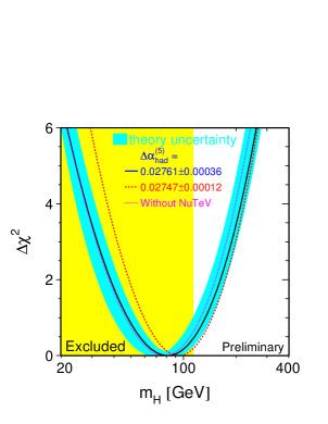
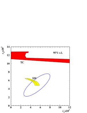
Figure 6: left: $\Delta\chi^{2}$ of the electroweak fit as a function of the Higgs mass. right: $\varepsilon$-parameters obtained from the LEP and SLD data compared to the Standard Model and to a technicolour model.

3.3 Prospects for the linear collider

A linear collider will be able to run with a luminosity of ${\cal L}\sim 5\cdot 10^{33}\rm\,cm^{-2}s^{-1}$ at energies close to the Z-pole [12]. With this luminosity it is possible to collect $10^{9}$ Z-decays in about 70 days of running. A similar luminosity should be possible close to the WW-threshold. In addition both beams have to be polarised with polarisations of ${\cal P}_{\rm{e}^{-}}=\pm 80\%$ and ${\cal P}_{\rm{e}^{+}}=\pm(40-60)\%$. This corresponds to an effective polarisation of ${\cal P}_{\rm{eff}}=\frac{{\cal P}_{\rm{e}^{+}}+{\cal P}_{\rm{e}^{-}}}{1+{\cal P}_{\rm{e}^{+}}{\cal P}_{\rm{e}^{-}}}\approx 91-95\%$. Additionally, the polarisation should be switchable randomly from train to train.

The parameters extracted from the Z-lineshape are already today largely systematics limited. For that reason only a modest improvement can be expected. Expressed in the minimally correlated observables $m_{\mathrm{Z}},\,\Gamma_{\mathrm{Z}},\,\sigma_{0}^{\rm{had}}=\frac{12\pi}{m_{\mathrm{Z}}^{2}}\frac{\Gamma_{e}\Gamma_{\mathrm{had}}}{\Gamma_{Z}^{2}},\,R_{\ell}=\frac{\Gamma_{\mathrm{had}}}{\Gamma_{l}}$ the precision of all scan observables is about 0.1%, apart from $m_{\mathrm{Z}}$ which is known to $2\cdot 10^{-5}$. At a linear collider it will probably not be possible to get an absolute calibration of the beam energy to the same level as it was possible at LEP. So $m_{\mathrm{Z}}$ will serve as calibration of the energy scale and thus cannot be improved.

However a relative calibration of the energy scale to $10^{-5}$ seems realistic, so that $\Delta\Gamma_{\mathrm{Z}}=1{\,\mathrm{Me\kern-1.00006ptV}}$ is within reach. With the much better detector planned in the linear collider designs [13] and the higher statistics to perform cross checks the systematics on the event selection should get improved by a factor of three relative to the best LEP experiment. This leads to a relative precision of $\Delta R_{\ell}/R_{\ell}=0.3\cdot 10^{-3}$. For the $\sigma_{0}^{\rm{had}}$ measurement the absolute luminosity is needed. The experimental systematics on this measurement might also decrease by a factor of three. However if the theoretical uncertainty of the small angle Bhabha cross section stays at its present value, the improvement in $\sigma_{0}^{\rm{had}}$ will be only 30% leading to $\Delta\sigma_{0}^{\rm{had}}/\sigma_{0}^{\rm{had}}=0.6\cdot 10^{-3}$. To achieve these precisions the beam-spread and the beamstrahlung need to be understood to a few percent. This task looks difficult but possible, however further studies are needed before a definite statement can be made.

The possible improvements in $\alpha_{s}(m_{\mathrm{Z}}^{2}),\,\Delta\rho_{\ell}$ and the number of light neutrino species ($N_{\nu}$), which can be seen as a general parameter for extra contributions to the invisible Z width are summarised in table 2. Typical improvements are a factor of two to three.

	LEP [2]	LC
$\alpha_{s}(m_{\mathrm{Z}}^{2})$	$0.1181\pm 0.0027$	$\pm 0.0009$
$\Delta\rho_{\ell}$	$(0.50\pm 0.10)\cdot 10^{-2}$	$\pm 0.05\cdot 10^{-2}$
$N_{\nu}$	$2.984\pm 0.008$	$\pm 0.004$

Table 2: Possible improvements in the physics quantities derived from the Z-lineshape after high luminosity Z-running at TESLA. For $\alpha_{s}$ and $\Delta\rho,N_{\nu}=3$ is assumed.

Large improvements are expected for the asymmetries which in general have low systematic errors, especially when polarised beams are involved. From the gain in statistics and effective polarisation relative to SLD [14] a factor of 50 smaller statistical error can be expected. For $A_{\rm{LR}}$ this corresponds to a relative error of $2\cdot 10^{-4}$. At present the relative error due to polarimetry is $0.5\%$ and it cannot be expected that a polarimeter at a linear collider will be much better than the one at SLD. The error decreases immediately by a factor of three when positron polarisation is available with the assumed value due to the error propagation from the single beam polarisations to the effective polarisation, but this is still by far not enough. However, the required precision can be obtained with the so called Blondel scheme[15].

In general the cross section $\mathrm{e}^{+}\mathrm{e}^{-}\rightarrow\rm{Z}\rightarrow\mathrm{f}\overline{\mathrm{f}}$ for polarised beams can be written as

$$\sigma\,=\,\sigma_{u}\left[1-{\cal P}_{\rm{e}^{+}}{\cal P}_{\rm{e}^{-}}+\mbox{$A_{\rm{LR}}$}({\cal P}_{\rm{e}^{+}}-{\cal P}_{\rm{e}^{-}})\right].$$ (1)

Measuring all four possible helicity combinations $A_{\rm{LR}}$ can be obtained without explicit knowledge of the polarisation:

$$\mbox{$A_{\rm{LR}}$}\,=\,\sqrt{\frac{(\sigma_{++}+\sigma_{-+}-\sigma_{+-}-\sigma_{--})(-\sigma_{++}+\sigma_{-+}-\sigma_{+-}+\sigma_{--})}{(\sigma_{++}+\sigma_{-+}+\sigma_{+-}+\sigma_{--})(-\sigma_{++}+\sigma_{-+}+\sigma_{+-}-\sigma_{--})}}\,,$$ (2)

where in $\sigma_{ij}$ $i$ denotes the sign of the positron- and $j$ the sign of the electron-polarisation. From an error analysis it turns out that only 10% of the luminosity needs to be spent on the small cross sections so that little luminosity is lost for other measurements and the statistical error increases only slightly due to the Blondel scheme.

In eq. (2) it is assumed that the absolute values of the polarisation for the positive and negative helicity states are equal. To verify this, or to get the relevant corrections, polarimeters like the one used at SLD are still needed. However the absolute calibration of the polarimeter analysing power, which is the dominant error in the polarimetry, drops out in the measurement. One possible source of uncertainty in this difference measurement could be a difference in luminosity of the electron-laser interaction for the two laser polarisations. This can be overcome by using two polarimeter channels with different analysing power.

The statistical error on $A_{\rm{LR}}$ with $10^{9}$ Z-decays will be $\Delta\mbox{$A_{\rm{LR}}$}=3\cdot 10^{-5}$. The variation of $A_{\rm{LR}}$ with the centre of mass energy is about ${\rm d}\mbox{$A_{\rm{LR}}$}/{\rm d}\sqrt{s}=2\cdot 10^{-2}/{\,\mathrm{Ge\kern-1.00006ptV}}$, so the beam energy relative to the Z-mass needs to be controlled to a precision of about 1 MeV. The amount of beamstrahlung expected in the high luminosity Z running changes $A_{\rm{LR}}$ by $\Delta\mbox{$A_{\rm{LR}}$}\,=\,9\cdot 10^{-4}$. It thus needs to be known to a precision of a few percent. If, however, the beamstrahlung in the Z-scan to calibrate the beam energy is the same as in the peak running it gets absorbed into an apparent shift of the calibration constants and basically no beamstrahl corrections for $A_{\rm{LR}}$ are needed.

It will be thus assumed that the linear collider can measure $A_{\rm{LR}}$ with a final precision of $10^{-4}$ corresponding to $\Delta\sin^{2}\!\theta_{\rm{eff}}^{\ell}=0.000013$

$\cal A_{\rm b}$ can be measured from the left-right-forward-backward asymmetry with similar methods as the ones used by LEP and SLD [16]. If the lepton and the jetcharge methods from LEP are taken as a reference a statistical error of $\Delta\mbox{$\cal A_{\rm b}$}\sim 5\cdot 10^{-4}$ is possible for both methods. Not to be completely dominated by light quark background the excellent b-tagging capabilities of the LC-detector need to be exploited. For the jetcharge analysis a b-tagging with $99\%$ purity is needed, which should be feasible with an efficiency of $75\%$. For the lepton-method a charm rejection of a factor of 50 is needed, which can be reached with $85\%$ efficiency.

For the lepton analysis the dominating error is then the statistical error from $\mathrm{b}\overline{\mathrm{b}}$-mixing ($\Delta\mbox{$\cal A_{\rm b}$}(\rm{mix})\approx 9\cdot 10^{-4}$). This error is of purely statistical nature and cannot be reduced. For the jetcharge method light quark background and hemisphere correlations will both contribute to the systematic uncertainty with $\Delta\mbox{$\cal A_{\rm b}$}\sim 10^{-3}$, so that, combining the two methods, a total error of $\Delta\mbox{$\cal A_{\rm b}$}=10^{-3}$ seems within reach.

Another Z-observable where significant progress can be achieved is $R_{\mathrm{b}}^{0}=\Gamma_{\mathrm{b}\overline{\mathrm{b}}}/\Gamma_{\mathrm{had}}$ which can be obtained with very small corrections from the cross section ratio $R_{\mathrm{b}}=\sigma_{\mathrm{b}\overline{\mathrm{b}}}/\sigma_{\rm{had}}$. At LEP this quantity is mainly limited by the understanding of the charm background, the background from gluon splitting into $\mathrm{b}\overline{\mathrm{b}}$ and hemisphere correlations due to QCD effects. These correlations arise from the energy dependence of the b-tag, because a gluon, emitted at a large angle, takes energy from both jets. With the LC-detector the charm background can be suppressed by a factor of four relative to the LEP analyses, simultaneously reducing the statistical error by a factor of 20. The better b-tagging and increased statistics should also allow for a improvement in the measurement of the gluon splitting. The energy dependence in the b-tag comes from the large multiple scattering contribution to the impact parameter resolution in the LEP detectors. At the LC detector the losses are mainly due to the cut on the invariant mass of the reconstructed particles at the secondary vertex. Since the invariant mass is a Lorenz-invariant quantity the energy dependence and thus the hemisphere correlations should be much smaller. For $R_{\mathrm{b}}$ a total improvement by about a factor of five can be expected.

The W-mass is presently known with a precision of 34 MeV. However LHC should be able to improve its precision to about 15 MeV[17]. The linear collider in principle has two possibilities to measure the mass of the W, with a scan of the W-pair-production threshold or reconstructing Ws at higher energy similar to LEP. The phase space suppression close to threshold is $\propto\beta$ for the neutrino t-channel exchange while it is $\propto\beta^{3}$ for the s-channel photon and Z-exchange. For that reason mainly the well known $\rm{We}\nu$-coupling enters in the prediction of the threshold cross section and the sensitivity to anomalous triple gauge couplings is very small. t-channel neutrino exchange is only present for left-handed electrons and right-handed positrons. With 100% beam polarisation for both beams the cross section can thus be enhanced by a factor of four for the right helicity combination and already with one beam being polarised switched off completely. The left-right asymmetry for the background is much smaller, so that polarisation can be used to enhance the signal/background ratio for one polarisation state and basically switch off the signal to measure the background for the opposite one.

A possible W-threshold scan has been simulated for TESLA spending $100\,\rm{fb}^{-1}$ close to $\sqrt{s}=161{\,\mathrm{Ge\kern-1.00006ptV}}$ corresponding to one year of running [18]. Efficiencies and backgrounds have been assumed to be the same as at LEP. With a total error of $0.25\%$ on the luminosity and on the selection efficiencies $m_{\mathrm{W}}$ can be measured with a total precision of $6{\,\mathrm{Me\kern-1.00006ptV}}$. If the efficiencies are left free in the fit, the error increases to only $7{\,\mathrm{Me\kern-1.00006ptV}}$ independent on the luminosity error. The achievable errors at the scan points are compared with the sensitivity to the W-mass in figure 7.

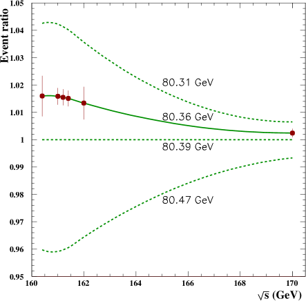
Figure 7: Sensitivity of the W-pair threshold scan to the W-mass. The vertical axis shows the ratio of the cross section to the predicted cross section for $m_{\mathrm{W}}=80.39{\,\mathrm{Ge\kern-1.00006ptV}}$. The error bars represent the expected errors for the scan described in the text.

With mass-reconstruction techniques using W-pair- and single-W-production at higher energies also a statistical error of a few MeV can be reached without dedicated luminosity. However it is not clear yet, if the systematics can be brought under control.

3.4 Interpretation of the precision measurements

To interpret the precision measurements one has to compare them to the model predictions at the loop level. In the theoretical prediction the uncertainties in all input parameters enter in the uncertainty of the prediction. The important parameters are:

• the running of $\alpha$ to the Z-mass. $\alpha(s)$ can be expressed as $\alpha(s)^{-1}=\left(1-\Delta\alpha_{\rm{lep}}(s)-\Delta\alpha_{\rm{had}}^{(5)}(s)-\Delta\alpha_{\rm{top}}(s)\right)\cdot\alpha^{-1}$. $\Delta\alpha_{\rm{lep}}(s)$ represents the leptonic loops which can be calculated reliably, while the hadronic loops, represented by $\Delta\alpha_{\rm{had}}^{(5)}(s)$ cause a large uncertainty. In principle they can be calculated from the cross section $\mathrm{e}^{+}\mathrm{e}^{-}\rightarrow\rm{hadrons}$ for energies up to the Z-mass using the optical theorem. However this leads to large uncertainties and everybody agrees to use perturbative QCD starting at some energy. However the energy from which on QCD can be used is under debate at the moment [19]. If data are used until well above the resonance region one obtains from the low energy data $\Delta\alpha_{\rm{had}}^{(5)}(m_{\mathrm{Z}}^{2})=(279.0\pm 4.0)\cdot 10^{-4}$  [20, 21] corresponding to an uncertainty in the Standard Model prediction of $\sin^{2}\!\theta_{\rm{eff}}^{\ell}$ of 0.00014 and 7 MeV in $m_{\mathrm{W}}$. However, the sensitivity to the details of the resonance region can be reduced significantly, if the low energy data is used to fit the coefficients of a QCD operator product expansion instead of integrating the total cross section. If the hadronic cross section is known to 1% up to the $\Upsilon$-resonances the uncertainties are $\Delta\sin^{2}\!\theta_{\rm{eff}}^{\ell}=0.000017$ and $\Delta m_{\mathrm{W}}=1{\,\mathrm{Me\kern-1.00006ptV}}$ [21].

• A top mass error of 1 GeV contributes an uncertainty of 0.000032 to the $\sin^{2}\!\theta_{\rm{eff}}^{\ell}$ prediction and 6 MeV to $m_{\mathrm{W}}$. At TESLA it should be possible to measure $m_{\mathrm{t}}$ to $\sim 100{\,\mathrm{Me\kern-1.00006ptV}}$, so that the top contribution to both observables will be negligible.

• A Z-mass error of 2 MeV results in a 0.000014 uncertainty of the $\sin^{2}\!\theta_{\rm{eff}}^{\ell}$ prediction, about the same size as the experimental error and the uncertainty from $\alpha(m_{\mathrm{Z}})$. For $m_{\mathrm{W}}$ the direct uncertainty is 2.5 MeV. However, the linear collider calibrates for all methods the W-mass with the Z-mass, so that the relevant observable is $m_{\mathrm{W}}/m_{\mathrm{Z}}$. In this case the error is smaller by a factor of three.

A 10% change in the Higgs mass will modify $\sin^{2}\!\theta_{\rm{eff}}^{\ell}$ by $0.000031$ and $m_{\mathrm{W}}$ by 6 MeV. When the Higgs is found by the time the measurements are done its mass will be known to better than 1% and thus not contribute to the uncertainty in the prediction. If the Higgs will not be found the data can be used to predict its mass to 5% accuracy. As an illustration figure 8 compares the Higgs mass fit of the LEP electroweak working group with the projected one after the LC precision measurements.

Figure 8: $\Delta\chi^{2}$ as a function of the Higgs mass for the electroweak precision data now and after the linear collider Z-factory running.

The precision measurements can also be used to constrain extensions of the Standard Model. As an example from the MSSM figure 9 [22] shows the area in $m_{\rm{A}}-\tan\beta$ that can be obtained from these data after certain assumptions on other SUSY-parameters, mainly affecting the stop-sector.

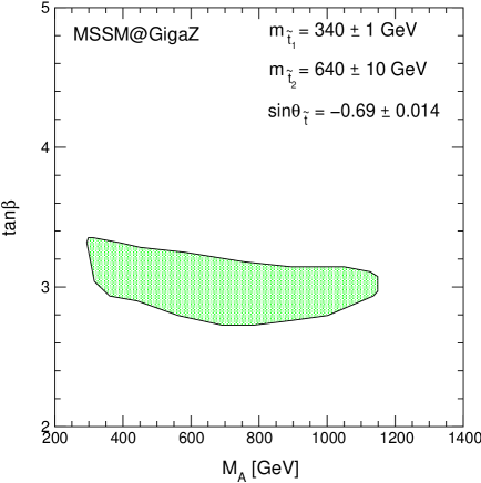
Figure 9: The region in the $m_{\rm{A}}-\tan\beta$ plane, allowed by $1\,\sigma$ errors by the measurements of $m_{\mathrm{W}}$ and $\sin^{2}\!\theta_{\rm{eff}}^{\ell}$: $m_{\mathrm{W}}=80.40{\,\mathrm{Ge\kern-1.00006ptV}}$, $\sin^{2}\!\theta_{\rm{eff}}^{\ell}=0.23138$, and by an LC measurement of $m_{\mathrm{H}}$: $m_{\mathrm{H}}=110{\,\mathrm{Ge\kern-1.00006ptV}}$. The other SUSY parameters including their uncertainties are given by $A_{\rm{b}}=-640\pm 60{\,\mathrm{Ge\kern-1.00006ptV}}$, $\mu=316\pm 1{\,\mathrm{Ge\kern-1.00006ptV}}$, $M_{2}=152\pm 2{\,\mathrm{Ge\kern-1.00006ptV}}$ and $m_{\tilde{g}}=496\pm 10{\,\mathrm{Ge\kern-1.00006ptV}}$.

Figure 10 shows the precision data in the $\varepsilon_{1}-\varepsilon_{3}$ plane for the present data and the LC-expectation with and without $m_{\mathrm{W}}$. The data are compared to the SM expectation with $m_{\mathrm{t}}=174{\,\mathrm{Ge\kern-1.00006ptV}}$ and $100{\,\mathrm{Ge\kern-1.00006ptV}}<m_{\mathrm{H}}<1{\,\mathrm{Te\kern-1.00006ptV}}$. Within the Standard Model the Higgs is already now significantly constrained because its trajectory is almost orthogonal to the long axis of the ellipse. Within many extensions of the SM, however, it is easy to generate an arbitrary $\varepsilon_{1}$ so that it is possible for basically any $m_{\mathrm{H}}$ to bring the prediction back into the ellipse. With the precision of the linear collider, especially including $m_{\mathrm{W}}$, the Higgs mass will be tightly constrained without any ambiguity from $\varepsilon_{1}$.

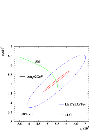
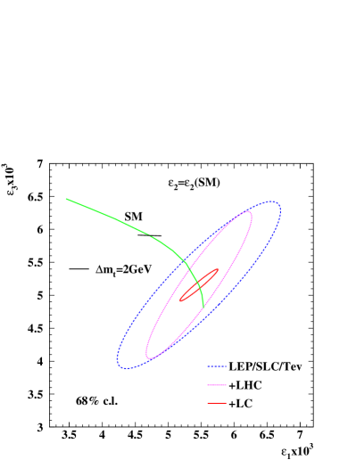
Figure 10: Sensitivity $\varepsilon_{1}-\varepsilon_{3}$ for the present data and the expectation at a linear collider. In the left plot $\varepsilon_{2}$ has been left free in the fit, equivalent to ignoring $m_{\mathrm{W}}$ in the $\varepsilon_{1}-\varepsilon_{3}$ fit. In the right plot $\varepsilon_{2}$ has been fixed to its SM-value. The line marked “SM” shows the SM prediction with $m_{\mathrm{t}}=174{\,\mathrm{Ge\kern-1.00006ptV}}$ and varying $m_{\mathrm{H}}$ from 70 GeV (lower end) to 1 TeV (upper end). The effect of an uncertainty in $m_{\mathrm{t}}$ of $2{\,\mathrm{Ge\kern-1.00006ptV}}$ is indicated. $\Delta m_{\mathrm{t}}=100{\,\mathrm{Me\kern-1.00006ptV}}$, expected from TESLA is inside the SM line width. For better comparability all central values gave been assumed to be on the SM prediction for $m_{\mathrm{H}}=100{\,\mathrm{Ge\kern-1.00006ptV}}$.

As an example of an application of the model independent analysis, figure 11 shows in the S-T plane the predictions from the 2-Higgs-Doublet Model (2HDM) for cases, where a light Higgs exists but cannot be seen, compared to the present data and the expectations from a linear collider [23]. Only a linear collider can distinguish between the Standard Model with a light Higgs and the 2HDM. One can also see, that for these sort of analyses the good precision in the W-mass is needed.

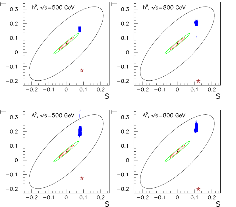
Figure 11: Prediction for S and T from the 2 Higgs doublet model with a light Higgs for the cases where no Higgs is found compared to the current electroweak data and the projection for Giga-Z. The star denotes the Standard Model prediction if the Higgs mass is $\sqrt{s}-100{\,\mathrm{Ge\kern-1.00006ptV}}$.

In summary, the properties of gauge bosons, namely the mass of the W and the fermion couplings of the Z will be highly sensitive to loop corrections. They will thus tightly constrain the SM, in case no new physics is found until then or help to measure the parameters of the new theory, if new phenomena are seen.

4 Measurements of the CKM matrix

The CKM matrix connects the weak eigenstates of down type quarks $(D_{1}^{\prime})$ to their mass eigenstates $(D_{i})$ [1]:

$$D_{i}^{\prime}\,=\,\sum_{j}V_{ij}D_{j}$$

The matrix has to be unitary to avoid flavour changing neutral currents on tree level, which have not been seen experimentally. For three flavours it can be parameterised by three angles and one complex phase, introducing CP violation. The coupling of an up-type quark $U_{i}$ and a down-type quark $D_{j}$ to the W-boson, normalised to the leptonic coupling of the W can thus be written as

$$g(U_{i},D_{j},W)=V_{ij}g(\ell,\nu,W).$$

Traditionally the CKM matrix elements are measured in weak meson decays. The absolute values of the elements can be measured from corresponding decay rates. Normally large event samples are available so that statistical errors are very small. However the hadronic matrix elements for the weak transitions are quite uncertain and the errors from this source are totally dominant. The phases of the elements only show up in interference patterns and are much harder to measure. A linear collider can contribute in three ways to the measurement of the CKM matrix elements:

• The elements $V_{{\rm t}i}$ can be accessed in top decays. This is discussed in chapter 3.

• The CP violating phases can be studied in B-decays in the Giga-Z running. The methods are essentially the same as at the $\mathrm{e}^{+}\mathrm{e}^{-}$ B-factories and the B-physics experiments at hadron machines, namely BTeV and LHCb and the expected precision is typically in between the lepton- and the hadron machines. A detailed discussion can be found in [24, 25, 26].

• The decay width of a W into a quark pair depends on the corresponding matrix element:

  $$\Gamma(W^{+}\rightarrow U_{i}\overline{D_{j}})=|V_{ij}|^{2}\Gamma(W^{+}\rightarrow\ell\overline{\nu})(1+{\cal C}_{\rm{QCD}}),$$

  where ${\cal C}_{\rm{QCD}}$ parameterises QCD corrections. This method will be described in some detail in the following [27].

The experimental problem in the measurement of the CKM matrix elements from W decays is the tagging of the quark flavours. For b- and c-quarks there exist well understood methods, tagging the decays of long lived b- and c-flavoured hadrons with the microvertex detector. Already at LEP and SLD these algorithms have been used successfully in many analyses and they are essential in Higgs physics at a linear collider. For light quarks no high efficiency, high purity methods exist. However it is known that the leading hadron in a jet often contains the primary quark so that it can be used for flavour tagging. The Z decay widths to b- and c-quarks and to the sum of all quarks are known with very good precision from LEP and SLD and they agree well with the Standard Model prediction. It is thus reasonable to assume that also the partial width to u-, d- and s-quarks agree with the prediction to the same precision. The tagging purities and efficiencies for all quarks in Z-decays using the microvertex methods for b- and c-quarks and leading hadrons for light quarks can thus be measured accurately in Z-running at the linear collider. Fragmentation properties depend only logarithmically on the energy scale. The extrapolation from the Z-mass scale to the W-mass scale can thus be done safely using the usual parton shower fragmentation models. Typically the efficiencies are 2% larger for the Ws. The only complication comes from the fact that, due to isospin invariance, the probability for a primary u- or d-quark to end up in a charged pion is about the same, making the fit to the Z-data unstable. However, because of charge conservation the W always has to decay in one up- and one down-type (anti-)quark. If, as an example, one quark from a W is tagged as charm the other one can be a down-quark, but not an up-quark. So the problem can be solved if the Z- and the W-data are fitted simultaneously with the tagging efficiencies and the W-branching ratios as free parameters, without introducing additional model dependence. Table 3 shows the obtainable efficiencies for light quarks using $\pi^{\pm},\,K^{\pm},\,K^{0}_{s},\,p$ and $\Lambda$.

	d	u	s
$\pi^{\pm}$	0.209	0.209	0.130
K±	0.056	0.074	0.122
p	0.015	0.025	0.020
K${}^{0}_{S}$	0.007	0.006	0.019
$\Lambda$	0.003	0.003	0.008

Table 3: Light quark tagging efficiencies of leading hadrons with $x_{p}>0.2$

For the analysis of the CKM-matrix all events containing W bosons can be used. Especially attractive, however, are single W events. The W in these events has on average a very small momentum so that the typical jet energies are close to those in Z-pole events. So in these events the extrapolation of the detector efficiencies, which vary strongly with energy, especially for the dE/dx measurement, is very small. Table 4 shows the sensitivity of a linear collider with $1500\,\rm{fb}^{-1}$ integrated luminosity compared to present and expected accuracy.

	current uncertainty	projected other	LC
$|V_{\mathrm{ud}}|$	$\pm$ 0.0008		$\pm$0.0028
$|V_{\mathrm{us}}|$	$\pm$0.0023		$\pm$0.0124
$|V_{\mathrm{ub}}|$	$\sim\pm$0.008	$\pm$0.0004	$\pm$0.011
$|V_{\mathrm{cd}}|$	$\pm$0.0016		$\pm$0.0072
$|V_{\mathrm{cs}}|$	$\pm$0.01		$\pm$0.0017
$|V_{\mathrm{cb}}|$	$\pm$0.0019	$\pm$0.0012	$\pm$0.0011

Table 4: Current [1] and projected [24] uncertainty of the CKM matrix elements compared to the LC measurement from W-decays.

A large gain can be obtained in $V_{\rm cs}$. However, if the unitarity of the CKM matrix is imposed, the present error in this element shrinks by more than one order of magnitude. Also in $V_{\rm cb}$ some progress is possible. This element is important for the interpretation of the CP-violation results in B-decays. If it is determined in B-decays the error is totally dominated by the theoretical uncertainty on the hadronic matrix elements, while in the determination from W-decays the error is statistical. The independent cross check is thus highly desirable.

5 Interactions amongst Gauge Bosons

The Standard Model predicts trilinear interactions between WWZ and WW$\gamma$, however there should be no interactions between neutral gauge bosons.

Single W production and W-pair production are sensitive to the triple gauge-boson couplings (TGC). In W-pair production the cross sections for neutrino t-channel exchange and $\gamma$,Z-s-channel exchange would rise individually with energy violating unitarity at some point. As demonstrated in figure 12 this rise is cancelled by the interference term, so that the resulting cross section shows the usual $1/s$ behaviour. For this reason W-pair production is extremely sensitive to the TGCs. To preserve the gauge cancellations, however, any anomalous coupling has to vanish for $\sqrt{s}\rightarrow\infty$. For the linear collider studies using W-pairs in principle this is not a problem, since the couplings are measured at a well defined scale. In the hadron collider studies the running of the couplings with the energy is often parameterised by a form factor $x^{\prime}=\frac{x}{\left(1+s/\Lambda^{2}\right)^{n}}$ with $n>0.5$ or $n>1$ depending on the type of coupling [17]. $\Lambda$ can be interpreted as the scale where the new physics, responsible for the anomalous couplings sets in, so that the effective parameterisation becomes meaningless above this scale.

Figure 12: W-pair production cross section for the different production processes separately, the interference and for the sum of all

Contrary to W-pair production the effective scale of single W production is always much lower than the centre of mass energy. The flux functions for radiating a W or a photon off the initial state electrons, peak at low energy so that the produced W is on average almost at rest.

In models where the gauge interactions remain weak they can be parameterised with a linear Lagrangian. Keeping terms with dimension up to six the most general Lagrangian for WWV (V=Z,$\gamma$) is

$$i{\cal L}_{eff}^{WWV} = g_{WWV}\cdot[$$

$$g_{1}^{V}V^{\mu}\left(W^{-}_{\mu\nu}W^{+\nu}-W^{+}_{\mu\nu}W^{-\nu}\right)+$$

$$\kappa_{V}W^{+}_{\mu}W^{-}_{\nu}V^{\mu\nu}+$$

$$\frac{\lambda_{V}}{m_{W}^{2}}V^{\mu\nu}W_{\nu}^{+\rho}W^{-}_{\rho\mu}+$$

$$ig_{5}^{V}\epsilon_{\mu\nu\rho\sigma}\left(\left(\partial^{\rho}W^{-\mu}\right)W^{+\nu}-W^{-\mu}\left(\partial^{\rho}W^{+\nu}\right)\right)V^{\sigma}+$$

$$ig_{4}^{V}W^{-}_{\mu}W^{+}_{\nu}\left(\partial^{\mu}V^{\nu}+\partial^{\nu}V^{\mu}\right)-$$

$$\frac{\tilde{\kappa}_{V}}{2}W^{-}_{\mu}W^{+}_{\nu}\epsilon^{\mu\nu\rho\sigma}V_{\rho\sigma}-$$

$$\frac{\tilde{\lambda}_{V}}{2m_{W}^{2}}W^{-}_{\rho\mu}W^{+\mu}_{\ \ \ \ \nu}\epsilon^{\nu\rho\alpha\beta}V_{\alpha\beta}]$$

with $V=\gamma,\,Z,\ g_{WW\gamma}=e,\ g_{WWZ}=e\cot\theta_{W}$ and $V_{\mu\nu}=\partial_{\mu}V_{\nu}-\partial_{\nu}V_{\mu}$.

Electromagnetic gauge invariance requires $g_{1}^{\gamma}(q^{2}=0)=1$ and $g_{5}^{\gamma}(q^{2}=0)=0$. In the Standard Model one has $g_{1}^{V}=\kappa_{V}=1$. All other couplings are equal to zero.

In term of these parameters the magnetic dipole moment of the W is given by $\mu_{W}=\frac{e}{2m_{W}}(1+\kappa_{\gamma}+\lambda_{\gamma})$ and the electric quadrupole-moment by $q_{W}=-\frac{e}{m_{W}^{2}}(\kappa_{\gamma}-\lambda_{\gamma})$.

From the terms in the effective Lagrangian the ones multiplied by $g_{1},\,\kappa$ and $\lambda$ are C- and P-conserving, the one proportional to $g_{5}$ violates C and P, however is CP-conserving and the ones with $g_{4},\,\tilde{\kappa}$ and $\tilde{\lambda}$ are CP-violating.

It is expected that deviations from the Standard Model should show up first in the C,P conserving couplings. At an $\mathrm{e}^{+}\mathrm{e}^{-}$-collider the process that is by far most sensitive to triple gauge couplings is W-pair production. However, if no beam polarisation is available, it is not possible to separate WW$\gamma$ and WWZ couplings with this process. If one requires that the anomalous couplings are C- and P-symmetric, preserve $SU(2)\times U(1)$ symmetry without adding operators of higher dimension and are not excluded by the LEP1 precision data one is left with the three couplings [28]:

$$\Delta g_{1}^{Z}$$

$$\Delta\kappa_{\gamma} = -\frac{\cos^{2}\theta_{W}}{\sin^{2}\theta_{W}}\left(\Delta\kappa_{Z}-\Delta g_{1}^{Z}\right)$$ (3)

$$\lambda_{\gamma} = \lambda_{Z}$$

Since the initial state couplings $\mathrm{e}^{+}\mathrm{e}^{-}\gamma$ and $\mathrm{e}^{+}\mathrm{e}^{-}\rm{Z}$ depend differently on the beam polarisation, polarised beams can be used to separate WW$\gamma$ and WWZ couplings, as demonstrated in figure 13. With enough statistics it is thus possible to measure the five C,P-conserving couplings simultaneously. The C,P-violating couplings can be separated easily by constructing C,P-odd observables.

Figure 13: Ratio of the differential cross section for W-pair production to the Standard Model prediction (a) and left-right asymmetry for this process (b) as a function of the W-production angle for anomalous $\kappa_{\gamma}$ or $\kappa_{Z}$.

If the triple gauge couplings are modified by 1-loop corrections one expects deviations of the order $g^{2}/16\pi^{2}\approx 2.7\cdot 10^{-3}$. As an example figure 14 [29] shows the expected effects on $\kappa_{\gamma}$ from loop corrections in the MSSM.

Figure 14: Expected effects on $\kappa_{\gamma}$ from MSSM loop corrections

5.1 Experimental procedures

In $\mathrm{e}^{+}\mathrm{e}^{-}\rightarrow\mathrm{W}^{+}\mathrm{W}^{-}$ anomalous gauge couplings show up in a modification of the differential cross section with respect to the scattering angle, where the modification depends on the W polarisation state. The W-polarisation is accessible from the decay angles of the W-decay products, so that in total five observables per event are available (see figure 15):

• the W production angle $\Theta$;

• the decay angles $\theta^{*}$ of the fermions with respect to the W flight direction in the W rest frame, sensitive to the longitudinal polarisation;

• the decay angles $\phi^{*}$ of the fermions in the W-beam plane, sensitive to transverse polarisations.

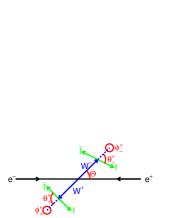
Figure 15: Observables available in a W-pair event

About 46% of the W-pairs decay into four quarks, 43% into two quarks a charged lepton and a neutrino and 11% into two charged leptons and two neutrinos. Neglecting initial state radiation and beamstrahlung the Ws are exactly back to back. In this approximation the axis of the W production in the mixed decays is measured from the decay products of the hadronically decaying W and the sign ambiguity is resolved by the charge of the lepton. For the leptonically decaying W both decay angles can be measured uniquely. For the hadronically decaying W the quark and the antiquark cannot be distinguished in general, so that the ambiguity $(\theta^{*},\phi^{*})\rightarrow(\pi-\theta^{*},\phi^{*}+\pi)$ remains. If the leptonically decaying W decays into $\tau\nu_{\tau}$ the resolution is worse, due to the additional neutrinos, but the measurement is still possible. For the fully hadronic W-pairs, even if the jet-pairing is done correctly, the decay angle ambiguities remain for both Ws and in addition the $\rm{W}^{+}$ and the $\rm{W}^{-}$ cannot be separated, so that these events are only of very limited use. The ambiguities can be solved partly by jetcharge techniques or c-tagging with some c-charge determination, but these methods have only a limited efficiency. If both W-bosons decay leptonically the full information can be reconstructed with a twofold ambiguity, if for the lepton-neutrino pairs the W mass is imposed. This works, however, only if no $\tau$ is involved, which is in about half of the events.

To analyse the data a binned analysis in a five-dimensional space is quite impractical. To circumvent this problem several methods are in use instead [28]:

Unbinned maximum likelihood fit:

In general an unbinned maximum likelihood fit is the statistically most powerful method. However it turns out that it is very difficult to apply corrections for detector effects, backgrounds etc., so that this fit has not been used for gauge coupling analyses on real data up to now.

Optimal observable methods:

If the differential cross section $d\sigma(q_{1},...q_{m})/d\Omega\ (\Omega=(\theta_{1},...\theta_{n}))$ is linear in the $m$ parameters, $q_{j}$, to be determined, i.e. the differential cross section can be written as

$$\frac{d\sigma}{d\Omega}=S_{0}(\Omega)+\sum_{j}S_{1,j}(\Omega)q_{j}$$

one can construct an optimal observable ${\cal O}_{j}(\Omega)=S_{1,j}(\Omega)/S_{0}(\Omega)$ for which it can be shown that the $q_{j}$ can be extracted in a statistically optimal way from the $\langle{\cal O}_{j}\rangle$ [30, 31]. If instead the distributions of the ${\cal O}_{j}(\Omega)$ are fitted, effects due to non linearity are accounted for automatically and for detector effects one can correct in the usual way. The ${\cal O}_{j}(\Omega)$ is just no longer exactly optimal, but when the non-linearity and detector corrections are small this is usually negligible. For $m<n$ one can thus reduce the number of parameters without a loss in statistical precision.

Spin density matrix:

The full information of the W pair cross section can be expressed as the product of the differential cross section $\partial\sigma/\partial\cos\Theta$ and the spin density matrix

$$\rho_{\tau_{-}\tau^{\prime}_{-}\tau_{+}\tau^{\prime}_{+}}(\cos\Theta)=\frac{\mathcal{F}_{\tau_{-}\tau_{+}}^{(\lambda)}\left(\mathcal{F}_{\tau^{\prime}_{-}\tau^{\prime}_{+}}^{(\lambda)}\right)^{\ast}}{\sum_{\tau_{+}\tau_{-}}\left|\mathcal{F}_{\tau_{-}\tau_{+}}^{(\lambda)}\right|^{2}},$$ (4)

where $\mathcal{F}_{\tau_{-}\tau_{+}}^{(\lambda)}$ is the amplitude for $\rm W^{-}\rm W^{+}$-pairs with W polarisations $\tau_{-}$ and $\tau_{+}$, respectively, and an initial electron polarisations of $\lambda$. In total this system has 81 density matrix elements where one is given by the normalisation

$$\sum_{\tau_{+}\tau_{-}}\rho_{\tau_{-}\tau_{-}\tau_{+}\tau_{+}}=1.$$

This number reduces to 35 elements in a CP conserving theory, as is described in [32]. Only little information is lost if the spin density matrix for single Ws is used in the analysis, neglecting spin correlations:

$$\rho_{\tau_{-}\tau_{-}^{\prime}}(\cos\Theta)=\sum_{\tau_{+}}\rho_{\tau_{-}\tau^{\prime}_{-}\tau_{+}\tau_{+}}.$$

$\rho_{\tau\tau^{\prime}}$ is hermitian, thus having 6 independent matrix elements. The diagonal elements, which are real, can be interpreted as the probability to find a W with helicity $\tau$. The imaginary parts of the off-diagonal elements vanish if CP is conserved.

Experimentally $\rho_{\tau\tau^{\prime}}$ can be obtained from

$$\rho_{\tau\tau^{\prime}}\frac{\partial\sigma}{\partial\cos\Theta}=\int\frac{\partial^{3}\sigma}{\partial\cos\Theta\partial\cos\theta^{*}\partial\phi^{*}}\Lambda_{\tau\tau^{\prime}}(\theta^{*},\phi^{*})d\cos\theta^{*}d\phi^{*}$$

The $\Lambda_{\tau\tau^{\prime}}$ are projection operators for the different helicity states, for example $\Lambda_{00}=2-5\cos^{2}\theta^{*}$. In this way the initial 5-dimensional parameter space can be reduced to 6 one-dimensional distributions.

5.2 Results at LEP and the Tevatron

Triple gauge couplings have already been measured at LEP2 and at the Tevatron. At LEP2 the measurements use the same processes as a linear collider will use. Since there one is closer to threshold the scales for W-pair and single W production are not so much different. However the single W production cross section is much smaller, so that also at LEP the dominant information comes from pair production. In $\mathrm{p}\bar{\mathrm{p}}$-collisions the most sensitive process is W$\gamma$-pair production, where the high $p_{t}$ photon is radiated off a W. Also WZ- and WW-pairs are analysed, however with a lower sensitivity than the W$\gamma$-pairs. $\mathrm{p}\bar{\mathrm{p}}$-collisions are thus mainly sensitive to WW$\gamma$ couplings. In general all measurements agree well with the Standard Model prediction with a precision of a few percent, so that in no realistic model a deviation is expected. As an example figure 16 shows the results of the three parameter fit in the $(\Delta g_{1}^{Z},-\Delta\kappa_{\gamma})$ and $(\Delta g_{1}^{Z}-\lambda_{\gamma})$ plane[2].

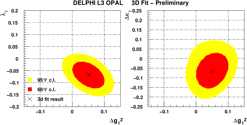
Figure 16: Result of the 3-parameter fit to the triple gauge couplings at DELPHI, L3 and OPAL.

5.3 Expectation from the linear collider

For the linear collider studies the spin density matrix formalism has been used which produces close to optimal results [33]. Fits have been performed for several numbers of free parameters with and without beam polarisation. As already said the symmetries of the couplings manifest themselves in the spin density matrix elements that are non-zero, so that the sets of couplings with different symmetries are basically measured without correlations between the sets. Table 5 shows the results of the different single parameter fits including the C or P violating couplings for $500\rm{fb}^{-1}$ at $\sqrt{s}=500{\,\mathrm{Ge\kern-1.00006ptV}}$ and $1000\rm{fb}^{-1}$ at $\sqrt{s}=800{\,\mathrm{Ge\kern-1.00006ptV}}$. For both cases an electron polarisation of $\pm 80\%$ and a positron polarisation of $\pm 60\%$ is assumed. Figure 17 shows the results of the five-parameter fit for $\sqrt{s}=800{\,\mathrm{Ge\kern-1.00006ptV}}$. Only the combinations with large correlations are shown.

coupling	$\sqrt{s}=500{\,\mathrm{Ge\kern-1.00006ptV}}$	$\sqrt{s}=800{\,\mathrm{Ge\kern-1.00006ptV}}$
C,P-conserving, $SU(2)\times U(1)$ relations:
$\Delta g^{\mathrm{Z}}_{1}$	$2.8$	$1.8$
$\Delta\kappa_{\gamma}$	$3.1$	$1.9$
$\lambda_{\gamma}$	$4.3$	$2.6$
C,P-conserving, no relations:
$\Delta g^{\mathrm{Z}}_{1}$	$15.5\phantom{0}$	$12.6\phantom{0}$
$\Delta\kappa_{\gamma}$	$3.3$	$1.9$
$\lambda_{\gamma}$	$5.9$	$3.3$
$\Delta\kappa_{\mathrm{Z}}$	$3.2$	$1.9$
$\lambda_{Z}$	$6.7$	$3.0$
not C or P conserving:
$g^{Z}_{5}$	$16.5\phantom{0}$	$14.4\phantom{0}$
$g^{Z}_{4}$	$45.9\phantom{0}$	$18.3\phantom{0}$
$\tilde{\kappa}_{Z}$	$39.0\phantom{0}$	$14.3\phantom{0}$
$\tilde{\lambda}_{Z}$	$7.5$	$3.0$

Table 5: Expected uncertainties of the single parameter fits to the different triple gauge couplings. For $\sqrt{s}=500{\,\mathrm{Ge\kern-1.00006ptV}}\ {\cal L}=500\rm{fb}^{-1}$ and for $\sqrt{s}=800{\,\mathrm{Ge\kern-1.00006ptV}}\ {\cal L}=1000\rm{fb}^{-1}$ has been assumed. For both energies ${\cal P}_{\rm{e}^{-}}=80\%$ and ${\cal P}_{\rm{e}^{+}}=60\%$ has been used.

Figure 17: $1\sigma$ and $95\%$ c.l. (2D) contours for $\Delta g^{\mathrm{Z}}_{1}$-$\Delta\kappa_{\mathrm{Z}}$, $\Delta g^{\mathrm{Z}}_{1}$-$\lambda_{Z}$, $\Delta\kappa_{\gamma}$-$\Delta\kappa_{\mathrm{Z}}$and $\lambda_{\gamma}$-$\lambda_{Z}$in the 5-parameter fit ($\sqrt{s}=800{\,\mathrm{Ge\kern-1.00006ptV}},\,{\cal L}=1000\rm{fb}^{-1},\,{\cal P}_{\rm{e}^{-}}=0.8,\,{\cal P}_{\rm{e}^{+}}=0.6$). For the combinations not shown the correlations are small.

Due to the large boost the resolution of the W-production angle is much better than at LEP. For the same reason the resolution in the decay angles is somewhat worse, however only sin and cos functions have to be distinguished here, so that the resolution is largely sufficient. In total the corrections due to detector effects are almost negligible and all experimental systematics are small. The radiative corrections however need to be known to significantly better than 1%. The beam polarisations can be measured from an extension of the Blondel scheme. The large forward peak of the cross section is dominated by neutrino t-channel exchange, so that its left-right asymmetry is very close to one, independent of the triple couplings. This region can be used to measure the electron polarisation directly from data, even if no positron polarisation is available.

Without beam polarisation only the fits without separating WW$\gamma$ and WWZ couplings are possible. For these fits the errors increase by about a factor of two.

The precision of $\kappa_{\gamma}$ for $\sqrt{s}=500{\,\mathrm{Ge\kern-1.00006ptV}}$ for example is $0.12\cdot(g^{2}/16\pi^{2})$. If this is compared to the expected loop corrections from the MSSM, shown in figure 14 one sees, that the gauge couplings can probe extensions of the Standard Model with sensitivities similar to the Z-fermion couplings.

Figure 18 compares the expected errors on $\kappa_{\gamma}$ and $\lambda_{\gamma}$ at the linear collider with those from other machines. Especially for $\kappa_{\gamma}$ the precision is much better than at the LHC. Since the dimension of the corresponding operator is lower for $\kappa$ than for $\lambda$ the suppression due to the high scale of new physics should be smaller. This parameter should thus be more sensitive to new effects for example from strong electroweak symmetry breaking.

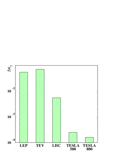
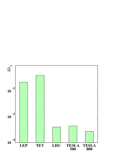
Figure 18: Comparison of $\Delta\kappa_{\gamma}$ and $\Delta\lambda_{\gamma}$ at different machines. For LHC and TESLA three years of running are assumed (LHC: $300\rm{fb}^{-1}$, TESLA $\sqrt{s}=500{\,\mathrm{Ge\kern-1.00006ptV}}$: $900\rm{fb}^{-1}$, TESLA $\sqrt{s}=800{\,\mathrm{Ge\kern-1.00006ptV}}$: $1500\rm{fb}^{-1}$).

Also the possibility to search for the neutral triple gauge couplings Z$\gamma\gamma$ and ZZ$\gamma$ has been studied [34]. However the possible limits are about an order of magnitude worse than predictions from loop effects in the Standard Model and expectations from the LHC. For this reason they will not be discussed further.

6 Strong electroweak symmetry breaking

If no Higgs boson exists electroweak interactions become strong at high energy and WW scattering violates unitarity at $\sqrt{s_{\rm{WW}}}=1.2{\,\mathrm{Te\kern-1.00006ptV}}$. The latest at this energy new physics has thus to set in, but with precision measurements it should be visible already at lower energies.

Strong electroweak symmetry breaking has already been discussed in detail in chapter 5[35], so only the features relevant to gauge boson physics will be repeated here. Without a Higgs the longitudinal degrees of freedom of the W and the Z become the Goldstone bosons of a strongly interacting theory and the low energy equivalence theorem (LET) [36, 37] relates longitudinal vector boson scattering to pion scattering at low energy. Concrete models typically predict resonances like the $\rho$ or the $\omega$ in QCD. However, as shown in figure 6 an exact copy of QCD is already excluded by the LEP/SLD precision data.

In a similar way as the $\rho$-resonance shows up in $\mathrm{e}^{+}\mathrm{e}^{-}\rightarrow\pi^{+}\pi^{-}$ also W-pair production should be sensitive to the strongly interacting scenario. In a model dependent analysis the amplitude for the production of two longitudinal Ws has been multiplied by a QCD like form factor assuming a resonance mass and width [38]. The LET is then the asymptotic value for high resonance masses. Figure 19 shows the expected sensitivity with $\sqrt{s}=800{\,\mathrm{Ge\kern-1.00006ptV}}$ and ${\cal L}=500\rm{fb}^{-1}$. Within the assumed model the LET and the SM model can clearly be distinguished and one is sensitive to resonance masses up to around $3{\,\mathrm{Te\kern-1.00006ptV}}$.

Figure 19: Sensitivity to a $\rho$ like resonance in W-pair production at $\sqrt{s}=800{\,\mathrm{Ge\kern-1.00006ptV}}$ and ${\cal L}=500\,\rm{fb}^{-1}$.

To analyse the data in a model independent way effects from strong electroweak symmetry breaking can be parameterised in an effective Lagrangian. From LEP1/SLD it is known that the $\rho$-parameter is approximately one and the small deviations can fully be described by Standard Model loop corrections, mainly from the top quark. It is therefore reasonable to keep only terms that conserve the custodial $SU(2)_{c}$ symmetry. Under this assumption the effective Lagrangian for the triple gauge couplings, keeping only terms of the lowest dimension, reads:

$$L_{TGC} = \frac{\alpha_{1}}{16\pi^{2}}\frac{gg^{\prime}}{2}B_{\mu\nu}\mathop{\mathrm{tr}}\Bigl{(}\sigma_{3}W^{\mu\nu}\Bigr{)}+$$

$$\frac{\alpha_{2}}{16\pi^{2}}\mathrm{i}g^{\prime}B_{\mu\nu}\mathop{\mathrm{tr}}\Bigl{(}\sigma_{3}V^{\mu}V^{\nu}\Bigr{)}+$$

$$\frac{\alpha_{3}}{16\pi^{2}}2\mathrm{i}g\mathop{\mathrm{tr}}\Bigl{(}W_{\mu\nu}V^{\mu}V^{\nu}\Bigr{)}$$

with $V_{\mu}=-\mathrm{i}g\frac{\sigma^{i}}{2}W^{i}_{\mu}+\mathrm{i}g^{\prime}\frac{\sigma^{3}}{2}B_{\mu}$. From a naive dimensional analysis one expects

$$\frac{\alpha_{i}}{16\pi^{2}}=\left(\frac{v}{\Lambda^{*}_{i}}\right)^{2}$$

with $v=246{\,\mathrm{Ge\kern-1.00006ptV}}$ and $\Lambda^{*}_{i}$ being the scale of the new physics. From unitarity arguments one needs $\Lambda^{*}\sim 3{\,\mathrm{Te\kern-1.00006ptV}}$ so that the $\alpha_{i}$ should be of ${\cal O}(1)$. The $\alpha_{i}$ can be expressed in terms of $g_{1}^{Z},\,\kappa_{\gamma},\kappa_{Z}$ as:

$$g_{1}^{Z} = 1+\frac{e^{2}}{\cos^{2}\theta_{W}(\cos^{2}\theta_{W}\!-\!\sin^{2}\theta_{W})}\frac{\alpha_{1}}{16\pi^{2}}+\frac{e^{2}}{\sin^{2}\theta_{W}\cos^{2}\theta_{W}}\frac{\alpha_{3}}{16\pi^{2}}$$

$$\kappa_{\gamma} = 1-\frac{e^{2}}{\sin^{2}\theta_{W}}\frac{\alpha_{1}}{16\pi^{2}}+\frac{e^{2}}{\sin^{2}\theta_{W}}\frac{\alpha_{2}}{16\pi^{2}}+\frac{e^{2}}{\sin^{2}\theta_{W}}\frac{\alpha_{3}}{16\pi^{2}}$$ (5)

$$\kappa_{Z} = 1+\frac{2e^{2}}{\cos^{2}\theta_{W}\!-\!\sin^{2}\theta_{W}}\frac{\alpha_{1}}{16\pi^{2}}-\frac{e^{2}}{\cos^{2}\theta_{W}}\frac{\alpha_{2}}{16\pi^{2}}+\frac{e^{2}}{\sin^{2}\theta_{W}}\frac{\alpha_{3}}{16\pi^{2}}$$

Unfortunately eq. 5 is singular in the blind direction

$$(\alpha_{1},\;\alpha_{2},\;\alpha_{3})_{{\rm blind}}\propto(\cos^{2}\theta_{W}-\sin^{2}\theta_{W},\;\cos^{2}\theta_{W},\;-\sin^{2}\theta_{W})$$

so that not all the $\alpha_{i}$ can be extracted from triple gauge couplings. However, $\alpha_{1}$ can also be constrained from the Z-pole data. Figure 20 shows the expected errors in the $(\alpha_{1},\alpha_{2},\alpha_{3})$ space for $\sqrt{s}=800{\,\mathrm{Ge\kern-1.00006ptV}},\,{\cal L}=100\,\rm{fb}^{-1},{\cal P}_{\rm{e}^{-}}=80\%$ and ${\cal P}_{\rm{e}^{+}}=60\%$ and from the Z-pole expectation at Giga-Z. Also the errors in $(\alpha_{2},\alpha_{3})$ for $\alpha_{1}=0$ and for the combination of the high- and low-energy data are shown. The errors translate into mass scale limits of $\Lambda^{*}_{i}\approx 10{\,\mathrm{Te\kern-1.00006ptV}}$ which are well above the unitarity limit of $3{\,\mathrm{Te\kern-1.00006ptV}}$.

Figure 20: Sensitivity to the effective couplings $\alpha_{1,2,3}$ from the measurement of the triple gauge couplings at a linear collider and from the Z-pole precision data. For the Z-pole constraint the outer region is without and the inner region with the accurate $m_{\mathrm{W}}$ measurement. In the lower right plot the $\alpha_{2}-\alpha_{3}$ plane with $\alpha_{1}=0$ or with the Z-pole constraint is shown.

In the description of the quartic couplings with an effective Lagrangian there are two operators that conserve $SU(2)_{c}$ and that do not contribute already to the triple couplings:

$$L_{QGC} = \frac{\alpha_{4}}{16\pi^{2}}\mathop{\mathrm{tr}}\Bigl{(}V_{\mu}V_{\nu}\Bigr{)}\mathop{\mathrm{tr}}\Bigl{(}V^{\mu}V^{\nu}\Bigr{)}+$$

$$\frac{\alpha_{5}}{16\pi^{2}}\mathop{\mathrm{tr}}\Bigl{(}V_{\mu}V^{\mu}\Bigr{)}\mathop{\mathrm{tr}}\Bigl{(}V_{\nu}V^{\nu}\Bigr{)}$$

Experimentally the quartic couplings are measured through processes as sketched im figure 1. Since the electron coupling to the W is about a factor of two larger than the one to the Z, the sensitive processes have two neutrinos in the final state. This means that the gauge bosons in the final state have to be fully reconstructed so that decay modes involving neutrinos cannot be used.

In principle there are three processes sensitive to $\alpha_{4}$ and $\alpha_{5}$:

$$\mathrm{e}^{+}\mathrm{e}^{-} \rightarrow \nu\nu\mathrm{W}^{+}\mathrm{W}^{-}$$

$$\mathrm{e}^{+}\mathrm{e}^{-} \rightarrow \nu\nu\rm{ZZ}$$

$$\rm{e}^{-}\rm{e}^{-} \rightarrow \nu\nu\rm{W}^{-}\rm{W}^{-}$$

The sensitivity for the three processes is similar with different dependence on the two couplings. However, since the luminosity for $\rm{e}^{-}\rm{e}^{-}$ is about an order of magnitude less than for $\mathrm{e}^{+}\mathrm{e}^{-}$ the sensitivity per unit of running time in this channel is significantly smaller. A large potential background to these processes is $\mathrm{e}^{+}\mathrm{e}^{-}\rightarrow\mathrm{e}^{+}\mathrm{e}^{-}\mathrm{W}^{+}\mathrm{W}^{-}$ proceeding via intermediate photons. To reject this process it is important that electrons can be vetoed in the detector down to the lowest possible angles. If the electrons escape in the beampipe the total transverse momentum of the two-W system has to be very small. The $\mathrm{e}^{+}\mathrm{e}^{-}\rightarrow\mathrm{e}^{+}\mathrm{e}^{-}\mathrm{W}^{+}\mathrm{W}^{-}$ events can then be rejected by a cut on the total transverse momentum. Unfortunately such a cut suppresses also the longitudinal W-pairs more than the transverse ones. Another important background process is $\mathrm{e}^{+}\mathrm{e}^{-}\rightarrow{\rm e}\nu{\rm WZ}$. This background is in principle smaller than $\mathrm{e}^{+}\mathrm{e}^{-}\rightarrow\mathrm{e}^{+}\mathrm{e}^{-}\mathrm{W}^{+}\mathrm{W}^{-}$, but because of the missing neutrino the transverse momentum cut doesn’t work. The process can only be separated from the signal if the energy flow resolution of the detector for hadronic jets is good enough to separate Ws and Zs. Another possibility to enhance the signal to background ratio is beam polarisation. Ws couple only to left-handed electrons and right-handed positrons while the electron-photon coupling is polarisation independent.

In a possible analysis signal events are first separated from the background and then analysed in terms of the quartic couplings. Variables sensitive to these couplings are:

• the VV (V=W,Z) centre of mass energy;

• the V production angle in the VV rest frame, to select hard VV-scattering;

• the V decay angles to select longitudinal Vs.

Figure 21 shows the sensitivity of the linear collider at $\sqrt{s}=800{\,\mathrm{Ge\kern-1.00006ptV}}$ for $\mathrm{e}^{+}\mathrm{e}^{-}\rightarrow\nu\nu\mathrm{W}^{+}\mathrm{W}^{-}$ and $\mathrm{e}^{+}\mathrm{e}^{-}\rightarrow\nu\nu\rm{ZZ}$ [39]. Due to the different dependence on the two parameters the combination of the two processes greatly reduces the error. The reach in $\Lambda^{*}$ is $\Lambda_{4}^{*}\approx 1.8{\,\mathrm{Te\kern-1.00006ptV}}$ and $\Lambda_{5}^{*}\approx 2.5{\,\mathrm{Te\kern-1.00006ptV}}$ for the two parameter fit increasing to $\Lambda_{4}^{*}\approx 2.9{\,\mathrm{Te\kern-1.00006ptV}}$ and $\Lambda_{5}^{*}\approx 4.9{\,\mathrm{Te\kern-1.00006ptV}}$ for one-parameter fits, just reaching the interesting region of $3{\,\mathrm{Te\kern-1.00006ptV}}$. The sensitivity increases strongly with the centre of mass energy. A factor of two in energy reduces the errors on $\alpha_{4,5}$ by almost an order of magnitude.

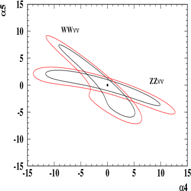
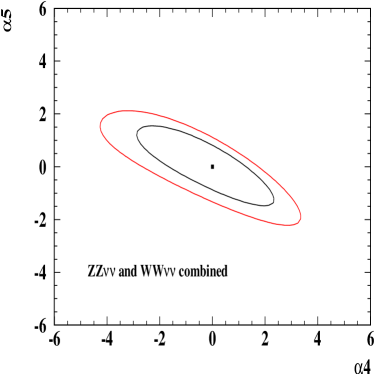
Figure 21: Sensitivity to $\alpha_{4}$ and $\alpha_{5}$ at $\sqrt{s}=800{\,\mathrm{Ge\kern-1.00006ptV}}$ from $\mathrm{e}^{+}\mathrm{e}^{-}\rightarrow\nu\nu\mathrm{W}^{+}\mathrm{W}^{-}$ and $\mathrm{e}^{+}\mathrm{e}^{-}\rightarrow\nu\nu\rm{ZZ}$. The inner and outer contours represent 68% and 90% c.l. (${\cal L}=1000\rm{fb}^{-1},\,{\cal P}_{\rm{e}^{-}}=0.8,\,{\cal P}_{\rm{e}^{+}}=0.4$).

The LHC can see resonances coupling to W-pairs up to masses of about 2 TeV [17]. If these resonances are vector-like a linear collider can easily measure their couplings in W-pair production (see e.g. fig. 19). If they are scalar or tensor particles some information on their couplings can be obtained from the measurement of $\alpha_{4}$ and $\alpha_{5}$. However if the electroweak symmetry is really broken in a strongly interacting scenario finally a linear collider with few TeV centre of mass energy will be needed.

7 Conclusions

With a linear collider our knowledge of the gauge boson properties can be increased largely in many respects. Running on the Z-pole and the W-threshold allows significant progress in the precision of the observables that are most sensitive to electroweak loop corrections: the fermionic couplings of the Z and the mass of the W. These measurements test the consistency of the then-Standard Model on the $10^{-4}$ level or allow to estimate still unknown parameters for example in Supersymmetry. Also some progress in the measurement of the CKM matrix in W-decays is possible, helping in the understanding of CP-violation.

The most important progress, however, can be reached in the measurement of interactions amongst gauge bosons. The gauge interactions are a necessary feature of a non Abelian gauge group and the structure of triple gauge couplings can be checked with a precision of few$\times 10^{-4}$. If a light Higgs exists a completely new class of precision observables sensitive to loop corrections is accessible. The gauge coupling measurements, however, are especially interesting if no light Higgs exists. With the triple boson couplings one is sensitive to new physics that has to be present at the TeV scale to avoid violations of unitarity at these energies. In addition one can measure for the first time the scattering of gauge bosons. Since this process is the one that violates unitarity the earliest it is the most obvious place to look for strong electroweak symmetry breaking effects. The disadvantage of this process is that the effective WW centre of mass energy is significantly lower than the $\mathrm{e}^{+}\mathrm{e}^{-}$ energy, but at $\sqrt{s}=800{\,\mathrm{Ge\kern-1.00006ptV}}$ one should already be able to see effects from new physics if no light Higgs exists, although with smaller sensitivity than with the triple boson couplings. At higher energies this process will become ideal to see new resonances.

In summary, gauge boson physics is an essential part of the linear collider physics program. In a scenario with a light Higgs it will be indispensable to consolidate the model and to change its status from a working hypotheses to a physics theory. If no Higgs is seen the measurement of three and four boson interactions will open up a window to the physics of electroweak symmetry breaking which might not be directly visible at any next generation collider.

References

- [1] Particle Data Group, K. Hagiwara et al, Phys. Rev. D66 (2002) 010001.
- [2] The LEP collaborations, A Combination of Preliminary Electroweak Measurements and Constraints on the Standard Model, CERN-EP/2002-091, hep-ex/0212036.
- [3] J. A. Aguilar-Saavedra et al., TESLA Technical Design Report Part III: Physics at an Linear Collider, DESY-01-011C.
- [4] T. Abe et al., Linear collider physics resource book for Snowmass 2001, hep-ex/0106055 (part 1), hep-ex/0106056 (part 2), hep-ex/0106057 (part 3), and hep-ex/0106058 (part 4).
- [5] ACFA Linear Collider Working Group Collaboration, K. Abe et al., Particle physics experiments at JLC, hep-ph/0109166.
- [6] A. Pukhov et al., CompHEP - a package for evaluation of Feynman diagrams and integration over multi-particle phase space. User’s manual for version 33., hep-ph/9908288; E.Boos and M.Dubinin, Single W-boson Production at Linear Colliders, hep-ph/9909214.
- [7] S. Jadach et al., Phys. Rev. D61 (2000) 113010;.
- [8] A. Denner et al., Phys. Lett. B475 (2000) 127; EPJdirect Vol. 2 C4 (2000) 1; Nucl. Phys. B587 (2000) 67.
- [9] M. Grünewald et al., Four Fermion Production in Electron Positron Collisions, report of the Four-fermion working group of the LEP2 Monte Carlo workshops, CERN, 1999/2000, hep-ph/0005309.
- [10] G. Altarelli et al., Phys. Lett. B349 (1995) 145.
- [11] M.E. Peskin, T. Takeuchi, Phys. Rev. D46 (1992), 381.
-
[12]
N. Walker TESLA luminosity at low centre of mass, talk presented at the
DESY/ECFA workshop Frascati, 8 - 10 November, 1998
http://wwwsis.lnf.infn.it/ecfadesy/index.htm.. - [13] G. Alexander et al., TESLA: The superconducting electron positron linear collider with an integrated X-ray laser laboratory. Technical design report. Part IV: A detector for TESLA, DESY-01-011D.
- [14] P. C. Rowson, D. Su, and S. Willocq, Ann. Rev. Nucl. Part. Sci. 51 (2001) 345–412.
- [15] A. Blondel, Phys. Lett. B202 (1988), 145.
- [16] K. Mönig, Rep. on Prog. in Phys. 61 (1998) 8, 999.
- [17] S. Haywood et al. Electroweak Physics, CERN-2000-004, 117.
- [18] G. Wilson, Precision Measurement of the W Mass with a Polarised Threshold Scan at a Linear Collider, LC-PHSM-2001-009.
- [19] J. Erler, Determinations of : Comparison and prospects, hep-ph/0111005.
- [20] S. Eidelmann and F. Jegerlehner, Zeit. Phys. C67 (1995), 585.
- [21] F. Jegerlehner, The effective fine structure constant at TESLA energies, hep-ph/0105283.
- [22] J. Erler et al., Phys. Lett. B486 (2000) 125.
- [23] J. Gunion, Do Precision Electroweak Constraints Guarantee collider Discovery of at least one Higgs Boson of a Type II two Higgs Doublet Model? talk given at LCWS2000, FNAL, October 24-28, 2000, hep-ph/0012199; P. Chankowski et al., hep-ph/0009271.
- [24] P.F Harrison, H.R. Quinn (eds.) The BaBar Physics Book, SLAC-R-504.
- [25] P. Ball et al., B Decays, CERN-2000-004, 305.
- [26] R. Hawkings, K. Mönig, EPJdirect C8 (1999) 1.
- [27] J. Letts, P. Mättig, Direct Determination of the CKM Matrix from Decays of W Bosons and Top Quarks at High Energy Colliders, LC-PHSM-2001-008.
- [28] G. Gounaris et al., Triple Gauge Boson Couplings CERN-96-01, Vol. 1, 525.
- [29] A. Arhrib et al. Radiative Contributions to TGC in the MSSM hep-ph/9603268.
- [30] D. Atwood and A. Soni, Phys. Rev. D45 (1992) 223.
- [31] M. Diehl, O. Nachtmann, Zeit. Phys. C62 (1994) 397.
- [32] M. Bilenky et al. Nucl. Phys. B409 (1993) 22.
- [33] W. Menges, A Study of Charged Current Triple Gauge Couplings at TESLA, LC-PHSM-2001-022.
- [34] J. Alcaraz, Neutral Gauge Boson Pair Production at Linear Colliders, Proceedings of the Worldwide Study on Physics and Experiments with Future Linear -colliders, Sitges, April 1999, Vol. 1, 431.
- [35] W. Killian, Dynamical Symmetry Breaking, to appear in Linear Collider Physics in the New Millennium, edited by K. Fujii, D. Miller and A. Soni, World Scientific, hep-ph/0303015.
- [36] M. Chanowitz and M. Gaillard, Nucl. Phys. B261 (1985) 379.
- [37] H. Veltman, Phys. Rev. D43 (1991) 2236.
- [38] T. L. Barklow, Strong symmetry breaking at e+ e- linear colliders, in Proc. of the APS/DPF/DPB Summer Study on the Future of Particle Physics (Snowmass 2001) ed. R. Davidson and C. Quigg, hep-ph/0112286.
- [39] R. Chierici, S. Rosati, M. Kobel. Strong electroweak symmetry breaking signals in WW scattering at TESLA, LC-PHSM-2000-038.