Abstract

The effect of the non-extensive form of statistical mechanics proposed by Tsallis on the formation of a quark-gluon plasma (QGP) has been recently investigated in ref. [1]. The results show that for small deviations ($\approx 10\%$) from Boltzmann-Gibbs (BG) statistics in the QGP phase, the critical temperature for the formation of a QGP does not change substantially for a large variation of the chemical potential. In the present effort we use the extensive $\kappa$-deformed statistical mechanics constructed by Kaniadakis to represent the constituents of the QGP and compare the results with ref. [1].

Substantial theoretical research has been carried out to study the phase transition between hadronic matter and the QGP. When calculating the QGP signatures in relativistic nuclear collisions, the distribution functions of quarks and gluons are traditionally described by BG statistics. In the past few years the non-extensive form of statistical mechanics proposed by Tsallis [2] has found applications in astrophysical self-gravitating systems [3], solar neutrinos [4], high energy nuclear collisions [5], cosmic microwave back ground radiation [6], high temperature superconductivity [7, 8] and many others. In these cases a small deviation of the Tsallis parameter, q, from 1 (BG statistics) reduces the discrepancies between experimental data and theoretical models. Recently Hagedorn’s [9] statistical theory of the momentum spectra produced in heavy ion collisions has been generalized using Tsallis statistics to provide a good description of $e^{+}e^{-}$ annihilation experiments [10, 11]. Furthermore, Walton and Rafelski [12] studied a Fokker-Planck equation describing charmed quarks in a thermal quark-gluon plasma and showed that Tsallis statistics were relevant. These results suggest that perhaps BG statistics may not be adequate in the quark-gluon phase.

It has been demonstrated [13, 14] that the non-extensive statistics can be considered as the natural generalization of the extensive BG statistics in the presence of long-range interactions, long-range microscopic memory, or fractal space-time constraints. It was suggested in [5] that the extreme conditions of high density and temperature in ultra relativistic heavy ion collisions can lead to memory effects and long-range color interactions. For this reason, the effect of the non-extensive form of statistical mechanics proposed by Tsallis on the formation of a QGP has been recently investigated in [1]. The results show that for small deviations ($\approx 10\%$) from BG statistics in the QGP phase, the critical temperature, $T_{c}$, for the formation of a QGP does not change substantially for a large variation of the chemical potential, $\mu$. This suggests that the critical temperature is to a large extent independent of the total number of baryons participating in the heavy ion collision responsible for the formation of the QGP.

Starting from the one parameter deformation of the exponential function $\exp_{\{\kappa\}}(x)=(\sqrt{1+\kappa^{2}x^{2}}+\kappa x)^{\frac{1}{\kappa}}$, a generalized statistical mechanics has been recently constructed by Kaniadakis [15], which reduces to the ordinary BG statistical mechanics as the deformation parameter, $\kappa$, approaches to zero. The difference between Tsallis and Kaniadakis statistics is the following: Tsallis statistics is non-extensive and reduces to BG statistics (extensive) as the Tsallis parameter, $q$, tends to one. On the other hand, Kaniadakis statistics is extensive and tends to BG statistics as the deformation parameter, $\kappa$, tends to zero. In the present effort we use the extensive $\kappa$-deformed statistical mechanics constructed by Kaniadakis to represent the constituents of the QGP and compare the results with [1].

For a particle system in the velocity space, the entropic density in $\kappa$-deformed statistics is given by [15]

$$\sigma_{\kappa}(\bar{n})=-\int d\bar{n}\>\ln_{\{\kappa\}}(\alpha\,\bar{n})\>,$$ (1)

where $\alpha$ is a real positive constant and $\kappa$ is the deformation parameter ($-1<\kappa<1$). As $\kappa\rightarrow 0$, the above entropic density reduces to the standard Boltzmann-Gibbs-Shannon (BGS) entropic density if $\alpha$ is set to be one. The entropy of the system, which is given by $S_{\kappa}=\int_{\Re}d^{n}v\,\sigma_{\kappa}(\bar{n})$, assumes the form

$$S_{\kappa}=-\frac{1}{2\>\kappa}\int_{\Re}d^{n}v\left(\frac{\alpha^{\kappa}}{1+\kappa}\,\bar{n}^{1+\kappa}-\frac{\alpha^{-\kappa}}{1-\kappa}\,\bar{n}^{1-\kappa}\right)$$ (2)

and reduces to the standard BGS entropy $S_{0}=-\int_{\Re}d^{n}v\>[\ln(\alpha\,\bar{n})-1]\>\bar{n}$ as the deformation parameter approaches to zero. This $\kappa$-entropy is linked to the Tsallis entropy $S_{q}^{(T)}$ through the following relationship [15]:

$$S_{\kappa}=\frac{1}{2}\frac{\alpha^{\kappa}}{1+\kappa}\,S_{1+\kappa}^{(T)}+\frac{1}{2}\frac{\alpha^{-\kappa}}{1-\kappa}\,S_{1-\kappa}^{(T)}+const.$$ (3)

For $\alpha$=1, the stationary statistical distribution corresponding to the entropy $S_{\kappa}$ can be obtained by maximizing the functional

$$\delta\>[S_{\kappa}+\int_{\Re}d^{n}v\>(\beta\,\mu\,\bar{n}-\beta\,\epsilon\,\bar{n})]=0.$$ (4)

In doing so, one obtains

$$\bar{n}=\exp_{\{\kappa\}}\beta(\mu-\epsilon)\>,$$ (5)

which reduces to the standard classical distribution as $\kappa\rightarrow 0$.

The entropic density for quantum statistics is given by [15]

$$\sigma_{\kappa}(\bar{n})=-\int d\bar{n}\>\ln_{\{\kappa\}}\left(\frac{\bar{n}}{1+\eta\,\bar{n}}\right)\,,$$ (6)

where $\eta$ is a real number. After maximization of the constrained entropy or, equivalently, after obtaining the stationary solution of the proper evolution equation associated to (6), one arrives to the following distribution [15]:

$$\bar{n}=\frac{1}{\exp_{\{\kappa\}}\beta(\epsilon-\mu)-\eta}\>,$$ (7)

where $\eta=1$ for $\kappa$-deformed Bose-Einstein distribution and $\eta=-1$ for $\kappa$-deformed Fermi-Dirac distribution.

If we use $\kappa$-deformed statistics to describe the entropic measure of the whole system, the distribution function can not , in general, be reduced to a finite, closed, analytical expression. For this reason, we use the $\kappa$-deformed statistics to describe the entropies of the individual particles, rather than of the system as a whole. The single particle distribution functions of quarks, antiquarks and gluons are given by

$$\bar{n}_{Q(\bar{Q})}=\left\{\sqrt{1+\kappa^{2}\,T^{-2}\,(k\mp\mu_{Q})^{2}}+\kappa\,T^{-1}\,(k\mp\mu_{Q})+1\right\}^{-1}$$ (8)

and

$$\bar{n}_{G}=\left\{\sqrt{1+\kappa^{2}\,T^{-2}\,k^{2}}+\kappa\,T^{-1}\,k-1\right\}^{-1}$$ (9)

respectively. In the limit $\kappa\rightarrow 0$ one recovers the corresponding BG quantum distributions for quarks, antiquarks and gluons (see (15) and (16) in [1]).

The expression for the pressure is given by

$$P_{QGP}=\frac{d_{Q}\,T}{2\,\pi^{2}}\int_{0}^{\infty}dk\,k^{2}\left(\frac{f_{Q}^{\kappa}-f_{Q}^{-\kappa}}{2\,\kappa}+\frac{f_{\bar{Q}}^{\kappa}-f_{\bar{Q}}^{-\kappa}}{2\,\kappa}\right)-$$

$$\frac{d_{G}\,T}{2\,\pi^{2}}\int_{0}^{\infty}dk\,k^{2}\,\left(\frac{f_{G}^{\kappa}-f_{G}^{-\kappa}}{2\,\kappa}\right)-B\,,$$ (10)

where

$$f_{Q(\bar{Q})}=1+\left[\sqrt{1+\kappa^{2}\,T^{-2}(k\mp\mu_{Q})^{2}}+\kappa\,T^{-1}(k\mp\mu_{Q})\right]^{-\frac{1}{\kappa}}\,,$$ (11)

$$f_{G}=1-\left[\sqrt{1+\kappa^{2}\,T^{-2}\,k^{2}}+\kappa\,T^{-1}\,k\right]^{-\frac{1}{\kappa}}$$ (12)

and B is the bag constant which is taken to be (210 MeV)⁴. Equation (10) reduces to (13) in [1] as $\kappa\rightarrow 0$.

The hadron phase is taken to contain only interacting nucleons and antinucleons and an ideal gas of massless pions. Since hadron-hadron interactions are of short-range, the BG statistics is successful in describing particle production ratios seen in relativistic heavy ion collisions below the phase transition. The interactions between nucleons is treated by means of a mean field approximation as in [1].

Assuming a first order phase transition between hadronic matter and QGP, one matches an equation of state (EOS) for the hadronic system and the QGP via Gibbs conditions for phase equilibrium:

$$P_{H}=P_{QGP},\hskip 28.45274ptT_{H}=T_{QGP},\hskip 28.45274pt\mu_{H}=\mu_{QGP}$$ (13)

With these conditions the pertinent regions of temperature, $T$, and baryon chemical potential, $\mu$, are shown in figure (1) for $\kappa$= 0, 0.23 and 0.29. For $\kappa$=0.23 (see fig. 2), we obtain essentially the same phase diagram as in the case of Tsallis statistics with $q$=1.1. Since both Tsallis and $\kappa$-deformed statistics are fractal in nature, we observe a similar flattening of the $T(\mu$) curves. This can be interpreted as follows: the formation of a QGP occurs at a critical temperature which is almost independent of the total number of baryons participating in heavy ion collision. The resulting insensitivity of the critical temperature to the total number of baryons presents a clear experimental signature for the existence of fractal statistics for the constituents of the QGP.

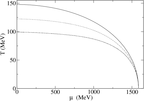
Figure 1: Phase transition curves between the hadronic matter and QGP for $\kappa$=0 (solid line), $\kappa$=0.23 (dotted line) and $\kappa$=0.29 (dashed line).

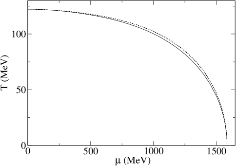
Figure 2: Phase transition curves between the hadronic matter and QGP for $\kappa$=0.23 (dashed line) and $q$=1.1 (solid line).

References

- [1] A.M. Teweldeberhan, H.G. Miller and R. Tegen, to be published in IJMPE.
- [2] C. Tsallis, J. Stat. Phys. 52 (1988) 479.
- [3] A.R. Plastino and A. Plastino, Phys. Lett. A 193 (1994) 251.
-
[4]
G. Kaniadakis, A. Lavagno and P. Quarati, Phys. Lett. B 369
(1996) 308,
G. Kaniadakis, A. Lavagno, M. Lissia and P. Quarati, Physica A 261 (1998) 359. - [5] W.M. Alberico, A. Lavagno and P. Quarati, Eur. Phys. J. C 12 (2000) 499 and Nucl. Phys. A 680 (2000) 94.
- [6] C. Tsallis, F.C.S. Barreto and E.D. Loh, Phys. Rev. E 52 (1995) 1447.
- [7] H. Uys, H.G. Miller and F.C. Khanna, Phys. Lett. A 289 (2001) 264.
- [8] Lizardo H.C.M. Nunes and E.V.L. de Mello, Physica A 305 (2002) 340.
- [9] R. Hagedorn, Nuovo Cimento, Suppl. 3 (1965) 147.
- [10] I. Bediaga, E. M. F. Curado and J. Miranda hep-th/9905 255
- [11] C. Beck, Physica A 286 (2000) 164.
- [12] D. B. Walton and J. Rafelski Phys. Rev Lett. 84 (2000) 31.
- [13] C. Tsallis, Phys. World 10 (1997) 42.
- [14] E.M.F Curado and C. Tsallis, J. Phys. A 24 (1991) L69.
- [15] G. Kaniadakis, Physica A 296 (2001) 405 and Phys. Rev. E 66 (2002) 056125.