Transition Form Factors between Pseudoscalar and Vector Mesons in Light-Front Dynamics

Abstract

We study the transition form factors between pseudoscalar and vector mesons using a covariant fermion field theory model in $(3+1)$ dimensions. Performing the light-front calculation in the $q^{+}=0$ frame in parallel with the manifestly covariant calculation, we note that the suspected nonvanishing zero-mode contribution to the light-front current $J^{+}$ does not exist in our analysis of transition form factors. We also perform the light-front calculation in a purely longitudinal $q^{+}>0$ frame and confirm that the form factors obtained directly from the timelike region are identical to the ones obtained by the analytic continuation from the spacelike region. Our results for the $B\rightarrow D^{*}l\nu_{l}$ decay process satisfy the constraints on the heavy-to-heavy semileptonic decays imposed by the flavor independence in the heavy quark limit.

I Introduction

In a recent analysis of spin-one form factors in light-front dynamics, we BCJ have shown that the zero-mode ZM complication can exist even in the matrix element of the plus current $J^{+}$. Using a simple but exactly solvable model of the spin-one system with the polarization vectors obtained from the light-front gauge ($\epsilon^{+}_{h=\pm 1}=0$), we found that the zero-mode contribution does not vanish in the helicity zero-to-zero amplitude. Neglecting the zero-mode contribution results in the violation of angular conditions BJ . There have been several recipes GK ; BH ; CCKP in spin-one systems to extract the invariant form factors from the matrix elements of the currents. Without taking into account the zero-mode contribution, however, these different receipes do not generate identical results in the physical form factors even if $J^{+}$ is used.

This indicates that the off-diagonal elements in the Fock-state expansion of the current matrix cannot be neglected for the helicity zero-to-zero amplitude even in reference frames where the plus component of the momentum transfer, $q^{+}$, vanishes. Since the factorization theorem in perturbative QCD (PQCD) relies essentially on the helicity zero-to-zero matrix element diagonal in the Fock-state expansion, the zero-mode contribution would complicate in principle the PQCD analysis of the spin-one (and higher spin) systems. Fortunately, our numerical computation indicates that the zero-mode contribution diminishes significantly in the high momentum transfer region where the PQCD analysis is applicable. Although the quantitative results that we found from our model calculation may differ in other models depending on the details of the dynamics in each model, the basic structure of our calculation is common to any other model calculations including the more phenomenological and realistic ones. Thus, we may expect the essential findings from our model calculation to be supported further by others. However, it doesn’t preclude the possibility that the zero-mode contribution may behave differently in different processes. Thus, it appears important to analyze a different process involving a spin-one system within the same model.

In this work, we analyze the transition form factors between pseudoscalar and vector mesons Jaus90 ; Jaus96 ; MS ; KT ; OXT ; CCH ; Jaus ; Jaus02 . These form factors can be measured in the semileptonic meson decay processes such as $B\to D^{*}l\nu_{l}$ and $B\to\rho l\nu_{l}$ produced from $B$-factories JC . The physical region of momentum transfer squared, $q^{2}$, for these processes (or form factors) is given by $4m_{l}^{2}\leq q^{2}\leq(M_{1}-M_{2})^{2}$, where $M_{1}$ and $M_{2}$ are the masses of the initial and final state mesons, respectively. This belongs to the timelike region, while the elastic spin-one meson form factors (i.e., $G_{E},G_{M},G_{Q}$) of for example the deuteron in the electron deuteron elastic scattering experiment can only be measured in the spacelike region, $q^{2}\leq 0$. Not long ago, the same transition form factors have been analyzed by Jaus Jaus using a light-like four-vector called $\omega$ $(\omega^{2}=0)$ and the admixture of a spurious $\omega$-dependent contribution was reported in the axial-vector form factor $A_{1}(q^{2})$ in the conventional light-front formulas. The removal of the $\omega$-dependence in the physical form factor amounts to the inclusion of the zero-mode contribution that we present in this work. However, the covariant formulation presented in our work should be intrinsically distinguished from the formulation involving $\omega$, since our formulation involves neither $\omega$ nor any unphysical form factor.

This paper is organized as follows. In Section II, we present the manifestly covariant calculation of the transition form factors between pseudoscalar and vector mesons using an exactly solvable Bethe-Salpeter(BS) model of ($3+1$)-dimensional fermion field theory. In Section III, we apply the light-front dynamics to calculate the same physical form factors. We separate the full amplitudes into the valence and nonvalence contributions and compare the results in the $q^{+}=0$ frame and the purely longitudinal $q^{+}>0$ frame. In the $q^{+}=0$ frame, we check whether the suspected zero-mode contribution exists or not within our analysis. In Section IV, we present the numerical results for the transition form factors making taxonomical decompositions of the full results into valence and nonvalence contributions. Conclusions follow in Section V. In Appendix A, we summarize the kinematics of the typical reference frames such as Drell-Yan-West (DWY), Breit (BRT), and target-rest frame (TRF) in the transition form factor analysis. In Appendix B, we present the manifestly covariant results of the electromagnetic form factors and decay constants of the pseudoscalar and vector mesons that are made of two unequal-mass constituents. These results are used in fixing the model parameters of our numerical analysis. In Appendices C and D, we present the more detailed formulae used in the discussion of subsections III.4 and III.5, respectively.

II Manifestly Covariant Computation

The Lorentz-invariant transition form factors $g$, $f$, $a_{+}$, and $a_{-}$ between a pseudoscalar meson with four-momentum $P_{1}$ and a vector meson with four-momentum $P_{2}$ and helicity $h$ are defined AW by the matrix elements of the electroweak current $J^{\mu}_{V-A}=V^{\mu}-A^{\mu}$ from the initial state $|P_{1};00\rangle$ to the final state $|P_{2};1h\rangle$:

$$\langle P_{2};1h|J^{\mu}_{V-A}|P_{1};00\rangle$$

$$\hskip 14.22636pt=ig(q^{2})\varepsilon^{\mu\nu\alpha\beta}\epsilon^{*}_{\nu}P_{\alpha}q_{\beta}-f(q^{2})\epsilon^{*\mu}$$

$$\hskip 14.22636pt-a_{+}(q^{2})(\epsilon^{*}\cdot P)P^{\mu}-a_{-}(q^{2})(\epsilon^{*}\cdot P)q^{\mu},{}$$ (1)

where the momentum transfer $q^{\mu}$ is given by $q^{\mu}=P_{1}^{\mu}-P_{2}^{\mu}$, $P=P_{1}+P_{2}$, and the polarization vector $\epsilon^{*}=\epsilon^{*}(P_{2},h)$ of the final state vector meson satisfies the Lorentz condition $\epsilon^{*}(P_{2},h)\cdot P_{2}=0$. While the form factor $g(q^{2})$ is associated with the vector current $V^{\mu}$, the rest of the form factors $f(q^{2})$, $a_{+}(q^{2})$, and $a_{-}(q^{2})$ are coming from the axial-vector current $A^{\mu}$. Thus, these transition form factors defined in Eq. (1) are often given by the following convention BSW ,

$$V(q^{2}) = (M_{1}+M_{2})g(q^{2}),$$

$$A_{1}(q^{2}) = {f(q^{2})\over{M_{1}+M_{2}}},$$

$$A_{2}(q^{2}) = -(M_{1}+M_{2})a_{+}(q^{2}),$$

$$A_{0}(q^{2}) = \frac{1}{2M_{2}}\biggl{[}f(q^{2})+(M_{1}^{2}-M_{2}^{2})a_{+}(q^{2})$$ (2)

$$+ q^{2}a_{-}(q^{2})\biggr{]},{}$$

where $M_{1}$ and $M_{2}$ are the initial and final meson masses, respectively.

The solvable model, based on the covariant Bethe-Salpeter(BS) model of ($3+1$)-dimensional fermion field theory, enables us to derive the transition form factors between pseudoscalar and vector mesons explicitly. The matrix element $\langle P_{2};1h|J^{\mu}_{V-A}|P_{1};00\rangle$ in this model is given by

$$\langle P_{2};1h|J^{\mu}_{V-A}|P_{1};00\rangle$$

$$=ig_{1}g_{2}\Lambda^{2}_{1}\Lambda^{2}_{2}\int\frac{d^{4}k}{(2\pi)^{4}}\frac{S^{\mu\nu}\epsilon^{*}_{\nu}(P_{2},h)}{D_{\Lambda_{1}}D_{m_{1}}D_{m}D_{m_{2}}D_{\Lambda_{2}}},{}$$ (3)

where $g_{1}$ and $g_{2}$ are the normalization factors which can be fixed by requiring both charge form factors of pseudoscalar and vector mesons to be unity at zero momentum transfer, respectively. To regularize the covariant fermion triangle-loop in ($3+1$) dimensions, we replace the point gauge-boson vertex $\gamma^{\mu}(1-\gamma_{5})$ by a non-local (smeared) gauge-boson vertex $\frac{{\Lambda_{1}}^{2}}{D_{\Lambda_{1}}}\gamma^{\mu}(1-\gamma_{5})\frac{{\Lambda_{2}}^{2}}{D_{\Lambda_{2}}}$, where $D_{\Lambda_{1}}=(P_{1}-k)^{2}-{\Lambda_{1}}^{2}+i\varepsilon$ and $D_{\Lambda_{2}}=(P_{2}-k)^{2}-{\Lambda_{2}}^{2}+i\varepsilon$, and thus the factor $({\Lambda_{1}}{\Lambda_{2}})^{2}$ appears in the normalization factor. $\Lambda_{1}$ and $\Lambda_{2}$ play the role of momentum cut-offs similar to the Pauli-Villars regularization BCJ1 . The rest of the denominators in Eq. (3), i.e., $D_{m_{1}}D_{m}D_{m_{2}}$, are coming from the intermediate fermion propagators in the triangle loop diagram and are given by

$$D_{m_{1}} = (P_{1}-k)^{2}-{m_{1}}^{2}+i\varepsilon,$$

$$D_{m} = k^{2}-m^{2}+i\varepsilon,$$

$$D_{m_{2}} = (P_{2}-k)^{2}-{m_{2}}^{2}+i\varepsilon.{}$$ (4)

Furthermore, the trace term in Eq. (3), $S^{\mu\nu}$, is given by

$$S^{\mu\nu}={\rm Tr}[(\not\!p_{2}+m_{2})\gamma^{\mu}(1-\gamma_{5})(\not\!p_{1}+m_{1})\gamma_{5}(-\not\!k+m)\Gamma^{\nu}],{}$$ (5)

where $m_{1}$, $m$, and $m_{2}$ are the masses of the constituents carrying the intermediate four-momenta $p_{1}=P_{1}-k$, $k$, and $p_{2}=P_{2}-k$, respectively. For the vector meson vertex, we shall use $\Gamma^{\mu}=\gamma^{\mu}$ in this section. While some modification of this simple vertex will be considered in Section III.5, our essential findings are not altered by that modification.

Using the familiar trace theorems, we find for $S^{\mu\nu}$:

$$S^{\mu\nu}= 4i\varepsilon^{\mu\nu\alpha\beta}[k_{\alpha}{P_{1}}_{\beta}(m-m_{2})+k_{\alpha}{P_{2}}_{\beta}(m_{1}-m)$$

$$+ {P_{1}}_{\alpha}{P_{2}}_{\beta}m]$$

$$+ 4g^{\mu\nu}[m_{1}k\cdot(k-P_{2})+m_{2}k\cdot(k-P_{1})$$

$$- m(k-P_{1})\cdot(k-P_{2})-{m_{1}}{m_{2}}m]$$

$$+ 4[2k^{\mu}k^{\nu}(m-m_{1})+k^{\mu}{P_{1}}^{\nu}(m_{2}-m)$$

$$+ k^{\mu}{P_{2}}^{\nu}(m_{1}-m)-k^{\nu}{P_{1}}^{\mu}(m_{2}+m)$$

$$+ k^{\nu}{P_{2}}^{\mu}(m_{1}-m)+({P_{1}}^{\mu}{P_{2}}^{\nu}+{P_{1}}^{\nu}{P_{2}}^{\mu})m],$$

where one should note that the ${P_{2}}^{\nu}$ terms will drop out once the polarization vector ${\epsilon}^{*}_{\nu}(P_{2},h)$ is multiplied into $S^{\mu\nu}$. We have checked our result with the one obtained by Jaus (see Eq. (4.10) of Ref. Jaus ) and found full agreement between the two results.

We then decompose the product of five denominators given in Eq. (3) into a sum of terms with three denominators only: i.e.,

$$\frac{1}{D_{\Lambda_{1}}D_{m_{1}}D_{m}D_{m_{2}}D_{\Lambda_{2}}} = \frac{1}{({\Lambda_{1}}^{2}-{m_{1}}^{2})({\Lambda_{2}}^{2}-{m_{2}}^{2})}\frac{1}{D_{m}}$$

$$\times \biggl{(}\frac{1}{D_{\Lambda_{1}}}-\frac{1}{D_{m_{1}}}\biggr{)}\biggl{(}\frac{1}{D_{\Lambda_{2}}}-\frac{1}{D_{m_{2}}}\biggr{)}.{}$$

Our treatment of the non-local smeared gauge-boson vertex remedies BCJ1 the conceptual difficulty associated with the asymmetry appearing if the fermion-loop were regulated by smearing the $q\bar{q}$ bound-state vertex. As discussed in our previous work BCJ1 ; BCJ , the two methods lead to different results for the calculation of the decay constants although they give the same result for the form factors. For example, our result BCJ doesn’t yield a zero-mode contribution to the vector meson decay constant while the asymmetric smearing of the hadronic vertex leads to the contamination from the zero-mode Jaus .

Once we reduce the five propagators into a sum of terms containing three propagators using Eq. (II), we use the Feynman parametrization for the three propagators, e.g.,

$$\frac{1}{D_{m_{1}}D_{m}D_{m_{2}}}$$

$$= \int^{1}_{0}dx\int^{1-x}_{0}dy\frac{2}{[D_{m}+(D_{m_{1}}-D_{m})x+(D_{m_{2}}-D_{m})y]^{3}}.$$

We then make a Wick rotation of Eq. (3) in $D$-dimensions to regularize the integral, since otherwise one looses the logarithmically divergent terms in Eq. (3). Following the above procedure, we finally obtain the Lorentz-invariant transition form factors as follows:

$$g(q^{2}) = -\frac{{\cal N}}{8\pi^{2}}\int^{1}_{0}dx\int^{1-x}_{0}dy[m_{1}x+m_{2}y+m(1-x-y)]C,$$

$$f(q^{2}) = \frac{{\cal N}}{8\pi^{2}}\int^{1}_{0}dx\int^{1-x}_{0}dy\biggl{\{}2(m_{1}-m+2m_{2})\ln\biggl{(}\frac{C_{\Lambda_{1}m_{2}}C_{m_{1}\Lambda_{2}}}{C_{\Lambda_{1}\Lambda_{2}}C_{m_{1}m_{2}}}\biggr{)}$$

$$+ \biggl{[}2(m_{1}+m_{2}-m)\{(x+y)(xM_{1}^{2}+yM_{2}^{2})-xyq^{2}\}-m_{1}\{2yM_{2}^{2}+x(M_{1}^{2}+M_{2}^{2}-q^{2})\}$$

$$- m_{2}\{2xM_{1}^{2}+y(M_{1}^{2}+M_{2}^{2}-q^{2})\}+m\{2xM_{1}^{2}+2yM_{2}^{2}+(x+y-1)(M_{1}^{2}+M_{2}^{2}-q^{2})\}-2m_{1}m_{2}m\biggr{]}C\biggr{\}},$$

$$a_{+}(q^{2}) = \frac{{\cal N}}{8\pi^{2}}\int^{1}_{0}dx\int^{1-x}_{0}dy[(x+y)\{2x(m-m_{1})+m_{2}-m\}+x(m_{1}-m_{2}-2m)+m]C,$$

$$a_{-}(q^{2}) = \frac{{\cal N}}{8\pi^{2}}\int^{1}_{0}dx\int^{1-x}_{0}dy[(x-y)\{2x(m-m_{1})+m_{2}-m\}-x(m_{1}+m_{2})-m]C,{}$$ (9)

where ${\cal N}=g_{1}g_{2}\Lambda^{2}_{1}\Lambda^{2}_{2}/({\Lambda_{1}}^{2}-{m_{1}}^{2})({\Lambda_{2}}^{2}-{m_{2}}^{2})$ and $C=(1/C_{\Lambda_{1}\Lambda_{2}}-1/C_{\Lambda_{1}m_{2}}-1/C_{m_{1}\Lambda_{2}}+1/C_{m_{1}m_{2}})$ with

$$C_{\Lambda_{1}\Lambda_{2}} = (1-x-y)(xM_{1}^{2}+yM_{2}^{2})+xyq^{2}$$

$$-(x\Lambda_{1}^{2}+y\Lambda_{2}^{2})-(1-x-y)m^{2},$$

$$C_{\Lambda_{1}m_{2}} = (1-x-y)(xM_{1}^{2}+yM_{2}^{2})+xyq^{2}$$

$$-(x\Lambda_{1}^{2}+ym_{2}^{2})-(1-x-y)m^{2},$$

$$C_{m_{1}\Lambda_{2}} = (1-x-y)(xM_{1}^{2}+yM_{2}^{2})+xyq^{2}$$

$$-(xm_{1}^{2}+y\Lambda_{2}^{2})-(1-x-y)m^{2},$$

$$C_{m_{1}m_{2}} = (1-x-y)(xM_{1}^{2}+yM_{2}^{2})+xyq^{2}$$ (10)

$$-(xm_{1}^{2}+ym_{2}^{2})-(1-x-y)m^{2}.{}$$

Note that the logarithmic term in $f(q^{2})$ is obtained from the dimensional regularization with the Wick rotation.

III Light-front calculation

It is native to the light-front analysis that a judicious choice of the current component is important for an effective computation of matrix elements. For the present work, we shall use only the plus-component of the current matrix element $\langle P_{2};1h|J^{\mu}_{V-A}|P_{1};00\rangle$ in the calculation of the transition form factors.

As we did in Ref. BCJ , the LF calculation for the trace term in Eq. (5) with plus current ($\mu=+$) can be separated into the on-shell propagating part $S^{+}_{\rm on}$ and the instantaneous part $S^{+}_{\rm inst}$ via

$${}\not\!p+m = (\not\!p_{\rm on}+m)+\frac{1}{2}\gamma^{+}(p^{-}-p^{-}_{\rm on})$$ (11)

as

$${}S^{+}_{h} = S^{+\nu}\epsilon^{*}_{\nu}(P_{2},h)=S^{+(h)}_{\rm on}+S^{+(h)}_{\rm inst},$$ (12)

where

$${}S^{+(h)}_{\rm on\;V-A} = -4i\varepsilon^{+\mu\nu\alpha}[m_{1}(p_{2\rm on})_{\mu}(k_{\rm on})_{\nu}-m_{2}(p_{1\rm on})_{\mu}(k_{\rm on})_{\nu}$$ (13)

$$\;\hskip 34.14322pt-m(p_{1\rm on})_{\mu}(p_{2\rm on})_{\nu}]\epsilon^{*}_{\alpha}$$

$$+4m_{1}[(k_{\rm on}\cdot\epsilon^{*})p^{+}_{2\rm on}+(p_{2\rm on}\cdot\epsilon^{*})k^{+}_{\rm on}$$

$$\;\hskip 34.14322pt-(p_{2\rm on}\cdot k_{\rm on})\epsilon^{*+}]$$

$$-4m_{2}[(k_{\rm on}\cdot\epsilon^{*})p^{+}_{1\rm on}-(p_{1\rm on}\cdot\epsilon^{*})k^{+}_{\rm on}$$

$$\;\hskip 34.14322pt+(p_{1\rm on}\cdot k_{\rm on})\epsilon^{*+}]$$

$$+4m[(p_{2\rm on}\cdot\epsilon^{*})p^{+}_{1\rm on}+(p_{1\rm on}\cdot\epsilon^{*})p^{+}_{2\rm on}$$

$$\;\hskip 34.14322pt-(p_{1\rm on}\cdot p_{2\rm on})\epsilon^{*+}]$$

$$-4m_{1}m_{2}m\epsilon^{*+},$$

and

$${}S^{+(h)}_{\rm inst\;V-A} = -4(k^{-}-k^{-}_{\rm on})m_{2}p^{+}_{1\rm on}\epsilon^{*+},$$ (14)

with $p_{1}=P_{1}-k$, $p_{2}=P_{2}-k$. The subscript (on) denotes the on-mass shell ($p^{2}=m^{2}$) quark momentum, i.e., $p^{-}=p^{-}_{\rm on}=(m^{2}+{\bf p}^{2}_{\perp})/p^{+}$. Note that the first term of $S^{+}_{\rm on}$ corresponds to the vector current matrix element and the rest to the axial-vector current matrix element. The instantaneous contribution $S^{+}_{\rm inst}$ comes only from the axial-vector current, i.e., $S^{+(h)}_{\rm inst\;V-A}=-S^{+(h)}_{\rm inst\;A}$.

The polarization vectors used in this analysis are given by

$${}\epsilon^{\mu}(\pm 1) = [\epsilon^{+},\epsilon^{-},\epsilon_{\perp}]=\biggl{[}0,\frac{2}{P^{+}_{2}}{\bf\epsilon}_{\perp}(\pm)\cdot{\bf P_{2\perp}},{\bf\epsilon}_{\perp}(\pm 1)\biggr{]},$$

$${\bf\epsilon}_{\perp}(\pm 1) = \mp\frac{(1,\pm i)}{\sqrt{2}},$$

$$\epsilon^{\mu}(0) = \frac{1}{M_{2}}\biggl{[}P^{+}_{2},\frac{{\bf P}^{2}_{2\perp}-M^{2}_{2}}{P^{+}_{2}},{\bf P}_{2\perp}\biggr{]}.$$ (15)

The traces in Eqs. (13) and (14) are then obtained as

$${}S^{+(h=1)}_{\rm on\;V} = \frac{2P^{+}_{1}}{\sqrt{2}}\varepsilon^{+-xy}\biggl{\{}q^{L}{\cal A}_{P}+k^{L}\;[\;(m-m_{2})(1-x)$$

$$+(m_{1}-m)(\alpha-x)+(m_{1}-m_{2})x\;]\biggr{\}},$$

$$S^{+(h=1)}_{\rm on\;A} = -\frac{4P^{+}_{1}}{\sqrt{2}}\biggl{\{}\frac{(\alpha-2x)}{\alpha}q^{L}{\cal A}_{P}$$

$$+k^{L}\;[\;(\alpha-2x)(m_{1}-m)-(m_{2}+m)\;]\biggr{\}},$$

$$S^{+(h=1)}_{\rm inst\;V} = S^{+(h=1)}_{\rm inst\;A}=0,$$ (16)

for the transverse polarization vector ($h=1$) and

$${}S^{+(h=0)}_{\rm on\;A} = \frac{4P^{+}_{1}}{x^{\prime}M_{2}}\biggl{\{}{\cal A}_{P}[\;x^{\prime}(1-x^{\prime})M^{2}_{2}+m_{2}m+x^{\prime 2}{\bf q}^{2}_{\perp}\;]$$

$$+{\bf k}^{2}_{\perp}(xm_{1}+m_{2}-xm)$$

$$+x^{\prime}{\bf k}_{\perp}\cdot{\bf q}_{\perp}[\;2x(m_{1}-m)+m_{2}+m\;]\biggr{\}},$$

$$S^{+(h=0)}_{\rm inst\;A} = \frac{4\alpha(P^{+}_{1})^{2}}{M_{2}}(1-x)m_{2}(k^{-}-k^{-}_{\rm on}),$$

for the longitudinal one ($h=0$), where

$$\alpha = P^{+}_{2}/P^{+}_{1}=1-q^{+}/P^{+}_{1},\;x=k^{+}/P^{+}_{1},\;x^{\prime}=x/\alpha,$$

$$q^{L} = q_{x}-iq_{y},\;k^{L}=k_{x}-ik_{y},$$

$${\cal A}_{P} = xm_{1}+(1-x)m.$$ (18)

Here, we used the ${\bf P}_{1\perp}=0$ frame. The (timelike) momentum transfer $q^{2}=(P_{1}-P_{2})^{2}$ is in general given by

$${}q^{2} = q^{+}q^{-}-{\bf q}^{2}_{\perp}=(1-\alpha)\biggl{(}M^{2}_{1}-\frac{M^{2}_{2}}{\alpha}\biggr{)}-\frac{{\bf q}^{2}_{\perp}}{\alpha}.$$ (19)

Defining the matrix element $\langle P_{2};1h|J^{+}_{V-A}|P_{1};00\rangle\equiv\langle J^{+}_{V-A}\rangle^{h}$ of the plus component of the V–A current in Eq. (3) as

$${}\langle J^{+}_{V-A}\rangle^{h}=ig_{1}g_{2}\Lambda^{2}_{1}\Lambda^{2}_{2}\int\frac{d^{4}k}{(2\pi)^{4}}\frac{(S^{+(h)}_{\rm on}+S^{+(h)}_{\rm inst})_{V-A}}{D_{\Lambda_{1}}D_{m_{1}}D_{m}D_{m_{2}}D_{\Lambda_{2}}},$$ (20)

one obtains the relations between the current matrix elements and the weak form factors as follows

$${}\langle J^{+}_{V}\rangle^{h=1} = -\frac{P^{+}_{1}}{\sqrt{2}}\varepsilon^{+-xy}q^{L}g(q^{2}),$$

$$\langle J^{+}_{V}\rangle^{h=0} = 0,$$ (21)

for the vector current and

$${}\langle J^{+}_{A}\rangle^{h=1} = \frac{P^{+}_{1}q^{L}}{\alpha\sqrt{2}}\biggl{[}(1+\alpha)a_{+}(q^{2})+(1-\alpha)a_{-}(q^{2})\biggr{]},$$

$$\langle J^{+}_{A}\rangle^{h=0} = \frac{\alpha P^{+}_{1}}{M_{2}}f(q^{2})+\frac{\alpha P^{+}_{1}}{2M_{2}}\biggl{(}M^{2}_{1}-\frac{M^{2}_{2}}{\alpha^{2}}+\frac{{\bf q}^{2}_{\perp}}{\alpha^{2}}\biggr{)}$$ (22)

$$\times \biggl{[}(1+\alpha)a_{+}(q^{2})+(1-\alpha)a_{-}(q^{2})\biggr{]},$$

for the axial-vector current.

III.1 Methods of extracting weak form factors

The extraction of weak form factors can be done in various ways. Among them, there are two popular ways of extracting the form factors, i.e., (1) the form factors are obtained in the spacelike region using the $q^{+}=0$ frame and then analytically continued to the timelike region by changing ${\bf q}_{\perp}$ to $i{\bf q}_{\perp}$, (2) the form factors are obtained by a direct timelike analysis using a $q^{+}>0$ frame. In this work, we shall analyze the form factors in both ways.

In the $q^{+}=0$ frame (i.e., $\alpha=1$) with the transverse polarization modes, one could extract the form factors $g(q^{2})$ and $a_{+}(q^{2})$ without including the zero-mode contributions as one can see from Eqs. (III) and (III). One could in principle obtain the form factor $f(q^{2})$ in the $q^{+}=0$ frame and the longitudinal polarization mode. In this case, it is important to check whether the zero-mode contribution exists or not by investigating the instantaneous part of the trace given by Eq. (III). In particular, as we discussed in Section I, the admixture of spurious $\omega$-dependent contributions was reported Jaus indicating a possible zero-mode contribution to the axial form factor $A_{1}(q^{2})$ which is essentially identical to $f(q^{2})$ modulo some constant factor (see Eq. (2)). As we shall show in Subsections III.4 and III.5, however, we find that the zero-mode contribution to the form factor $f(q^{2})$ does not exist in our analysis.

Using only the plus current $J_{V-A}^{+}$ in the $q^{+}=0$ frame, it is not possible to extract the form factor $a_{-}(q^{2})$. On the other hand, if one chooses a $q^{+}>0$ frame, specifically a purely longitudinal momentum frame where the momentum transfer is given by

$${}q^{2} = q^{+}q^{-}=(1-\alpha)\biggl{(}M^{2}_{1}-\frac{M^{2}_{2}}{\alpha}\biggr{)},$$ (23)

one can extract all four form factors by using only the plus-current. We compute them all in this purely longitudinal momentum frame including the nonvalence contributions for the matrix elements. This frame corresponds to the case $\theta=0$ or $\pi$ in the TRF and BRT frames summarized in Appendix A.

For this particular choice of the purely longitudinal frame, there are two solutions of $\alpha$ for a given $q^{2}$, i.e.,

$${}\alpha_{\pm}=\frac{M_{2}}{M_{1}}\biggl{[}\frac{M^{2}_{1}+M^{2}_{2}-q^{2}}{2M_{1}M_{2}}\pm\sqrt{\biggl{(}\frac{M^{2}_{1}+M^{2}_{2}-q^{2}}{2M_{1}M_{2}}\biggr{)}^{2}-1}\biggr{]},$$ (24)

where the $+(-)$ sign in Eq. (24) corresponds to the daugther meson recoiling in the positive(negative) $z$-direction relative to the parent meson. At zero recoil ($q^{2}=q^{2}_{\rm max}$) and maximum recoil ($q^{2}=0$), $\alpha_{\pm}$ are given by

$${}\alpha_{+}(q^{2}_{\rm max}) = \alpha_{-}(q^{2}_{\rm max})=\frac{M_{2}}{M_{1}},$$

$$\alpha_{+}(0) = 1,\;\;\alpha_{-}(0)=\biggl{(}\frac{M_{2}}{M_{1}}\biggr{)}^{2}.$$ (25)

The form factors are of course independent of the recoil directions ($\alpha_{\pm}$) if the nonvalence contributions are added to the valence ones. As one can see from Eqs. (III) and (III), however, one should be careful in setting ${\bf q}_{\perp}=0$ to get the results in this frame. One cannot simply set ${\bf q}_{\perp}=0$ from the start, but may set it to zero only after the form factors are extracted.

While the form factor $g(q^{2})$ in the $q^{+}>0$ frame can be obtained directly from Eq. (III), the form factor $f(q^{2})$ can be obtained only after $a_{\pm}(q^{2})$ are calculated.

To illustrate this, we define

$${}\langle J^{+}_{A}\rangle^{h=1}|_{\alpha=\alpha_{\pm}} \equiv \frac{P^{+}_{1}q^{L}}{\sqrt{2}}I^{+}_{A}(\alpha_{\pm}),$$ (26)

and obtain from Eq. (III)

$${}a_{+}(q^{2}) = \frac{\alpha_{+}(1-\alpha_{-})I^{+}_{A}(\alpha_{+})-\alpha_{-}(1-\alpha_{+})I^{+}_{A}(\alpha_{-})}{2(\alpha_{+}-\alpha_{-})},$$

$$a_{-}(q^{2}) = -\frac{\alpha_{+}(1+\alpha_{-})I^{+}_{A}(\alpha_{+})-\alpha_{-}(1+\alpha_{+})I^{+}_{A}(\alpha_{-})}{2(\alpha_{+}-\alpha_{-})},$$

and

$${}f(q^{2}) = \frac{M_{2}}{\alpha P^{+}_{1}}\langle J^{+}_{A}\rangle^{h=0}-\frac{1}{2}\biggl{(}M^{2}_{1}-\frac{M^{2}_{2}}{\alpha^{2}}\biggr{)}$$ (28)

$$\times\biggl{[}(1+\alpha)a_{+}(q^{2})+(1-\alpha)a_{-}(q^{2})\biggr{]}.$$

III.2 Valence contribution to $\langle J^{+}_{V-A}\rangle^{h}$

In the valence region $0<k^{+}<P^{+}_{2}$, the pole $k^{-}=k^{-}_{\rm on}=(m^{2}+{\bf k}^{2}_{\perp}-i\varepsilon)/k^{+}$ (i.e., the spectator quark) is located in the lower half of the complex $k^{-}$-plane. Thus, the Cauchy integration formula for the $k^{-}$-integral in Eq. (20) gives

$${}\langle J^{+}_{V-A}\rangle^{h}_{\rm val} = \frac{g_{1}g_{2}\Lambda^{2}_{1}\Lambda^{2}_{2}}{2(2\pi)^{3}}\int^{\alpha}_{0}\frac{dx}{x(1-x)^{2}(1-x^{\prime})^{2}}\int d^{2}{\bf k}_{\perp}\frac{S^{+(h)}_{\rm on\;V-A}}{(M^{2}_{1}-M^{2}_{0})(M^{2}_{1}-M^{2}_{\Lambda_{1}})(M^{2}_{2}-M^{\prime 2}_{0})(M^{2}_{2}-M^{\prime 2}_{\Lambda_{2}})},$$ (29)

where

$${}M^{2}_{0} = \frac{{\bf k}^{2}_{\perp}+m^{2}_{1}}{1-x}+\frac{{\bf k}^{2}_{\perp}+m^{2}}{x},$$

$$M^{\prime 2}_{0} = \frac{{\bf k^{\prime}}^{2}_{\perp}+m^{2}_{2}}{1-x^{\prime}}+\frac{{\bf k^{\prime}}^{2}_{\perp}+m^{2}}{x^{\prime}},$$ (30)

and $M^{2}_{\Lambda_{1}}=M^{2}_{0}(m_{1}\to\Lambda_{1})$, $M^{\prime 2}_{\Lambda_{2}}=M^{\prime 2}_{0}(m_{2}\to\Lambda_{2})$ with ${\bf k^{\prime}}_{\perp}={\bf k}_{\perp}+x^{\prime}{\bf q}_{\perp}$. Note that there is no instantaneous contribution in the valence region. From Eqs. (III) and (III), we obtain the valence contribution to $g(q^{2})$ as follows

$${}g(q^{2})_{\rm val} = -\frac{g_{1}g_{2}\Lambda^{2}_{1}\Lambda^{2}_{2}}{\alpha(2\pi)^{3}}\int^{\alpha}_{0}\frac{dx}{x(1-x)^{2}(1-x^{\prime})^{2}}\int d^{2}{\bf k}_{\perp}\frac{1}{(M^{2}_{1}-M^{2}_{0})(M^{2}_{1}-M^{2}_{\Lambda_{1}})(M^{2}_{2}-M^{\prime 2}_{0})(M^{2}_{2}-M^{\prime 2}_{\Lambda_{2}})}$$ (31)

$$\times\biggl{\{}{\cal A}_{P}+\frac{{\bf k}_{\perp}\cdot{\bf q}_{\perp}}{{\bf q}^{2}_{\perp}}\;[\;(m-m_{2})(1-x)+(m_{1}-m)(\alpha-x)+(m_{1}-m_{2})x\;]\biggr{\}}.$$

While Eq. (31) accounts only for the valence contribution in the $q^{+}>0$ frame, it is the exact solution in the $q^{+}=0$ (i.e., $\alpha=1$) frame due to the absence of the zero-mode contribution. Here, we should note the discrepancy between Ref. Jaus90 and Refs. OXT ; CCH for the calculation of the $g(q^{2})$ form factor. For the simple vector meson vertex of $\Gamma^{\mu}=\gamma^{\mu}$, our result is the same as Ref. Jaus90 but different from Refs. OXT ; CCH . The authors of Refs. OXT ; CCH claimed to compute the “$+$” component of the vector current (see for instance Eq. (2.75) in  CCH ). However, they indeed used the “$-$” component of the current instead of the “$+$” one. In their computation they used the coefficient of $\epsilon_{+-xy}$ which corresponds to $\gamma^{-}$ for the electroweak current vertex rather than the coefficient of $\epsilon_{-+xy}$(or equivalently $\epsilon^{+-xy}$) that corresponds to the plus current. This difference in choosing the component of the current caused the discrepancy between the results of Ref. Jaus90 and Refs. OXT ; CCH . It is well known BCJ1 that the minus current contains zero-mode contributions.

In the $q^{+}=0$ frame, the valence contribution to $a_{+}(q^{2})$ is the exact solution, again due to the absence of the zero-mode contribution. The result is obtained from Eqs. (III) and (III) as

$${}a_{+}(q^{2})|_{q^{+}=0} = -\frac{g_{1}g_{2}\Lambda^{2}_{1}\Lambda^{2}_{2}}{(2\pi)^{3}}\int^{1}_{0}\frac{dx}{x(1-x)^{4}}\int d^{2}{\bf k}_{\perp}\frac{1}{(M^{2}_{1}-M^{2}_{0})(M^{2}_{1}-M^{2}_{\Lambda_{1}})(M^{2}_{2}-M^{\prime 2}_{0})(M^{2}_{2}-M^{\prime 2}_{\Lambda_{2}})}$$ (32)

$$\times\biggl{\{}(1-2x){\cal A}_{P}+\frac{{\bf k}_{\perp}\cdot{\bf q}_{\perp}}{{\bf q}^{2}_{\perp}}\;[\;(1-2x)m_{1}-m_{2}-2(1-x)m\;]\biggr{\}}.$$

As we have shown in the present subsection, III.2, the two form factors $g(q^{2})$ and $a_{+}(q^{2})$ can be computed in the $q^{+}=0$ frame. The form factor $f(q^{2})$ can also be computed in the same frame, as we discussed in the last subsection III.1. The lack of a zero-mode contribution to $f(q^{2})$ is discussed in the subsections III.4 and III.5. Before we discuss this point, we first complete the presentation of the matrix element, i.e.,

$${}\langle J^{+}_{V-A}\rangle^{h} = \langle J^{+}_{V-A}\rangle^{h}_{\rm val}+\langle J^{+}_{V-A}\rangle^{h}_{\rm nv},$$ (33)

by computing the nonvalence contribution $\langle J^{+}_{V-A}\rangle^{h}_{\rm nv}$ in the next subsection, III.3 for an arbitrary $q^{+}$(or $\alpha$) value. The nonvalence contribution is necessary to compute the form factors in the purely longitudinal $q^{+}>0$ frame. It is confirmed in our numerical results (Section IV) that the values of the calculated form factors in the $q^{+}=0$ frame are identical to those in the purely longitudinal $q^{+}>0$ frame, as they should be when the nonvalence contribution is added to the valence one. In the purely longitudinal $q^{+}>0$ frame, we shall use Eqs. (III.1) and (28) to obtain the form factors $a_{\pm}(q^{2})$ and $f(q^{2})$, while the form factor $g(q^{2})$ can be obtained directly from Eq. (III).

III.3 Nonvalence contribution to $\langle J^{+}_{V-A}\rangle^{h}$

In the nonvalence region $P^{+}_{2}<k^{+}<P^{+}_{1}$, the poles are at $k^{-}=k^{-}_{m_{1}}\equiv P^{-}_{1}+[m^{2}_{1}+({\bf k}_{\perp}-{\bf P}_{1\perp})^{2}-i\varepsilon]/(k^{+}-P^{+}_{1})$ (from the struck quark propagator) and $k^{-}=k^{-}_{\Lambda_{1}}\equiv P^{-}_{1}+[\Lambda^{2}_{1}+({\bf k}_{\perp}-{\bf P}_{1\perp})^{2}-i\varepsilon]/(k^{+}-P^{+}_{1})$ (from the smeared quark-photon vertex), and are located in the upper half of the complex $k^{-}$-plane.

When we do the Cauchy integration over $k^{-}$ to obtain the LF time-ordered diagrams, we use Eq. (II) to avoid the complexity of treating double $k^{-}$-poles and obtain

$${}\langle J^{+}_{V-A}\rangle^{h}_{\rm nv} = \frac{{\cal N}}{2(2\pi)^{3}}\int^{1}_{\alpha}\frac{dx}{xx^{\prime\prime}(x-\alpha)}\int d^{2}{\bf k}_{\perp}\biggl{\{}\frac{S^{+(h)}_{\rm on}+S^{+(h)}_{\rm inst}(k^{-}=k^{-}_{\Lambda_{1}})}{(M^{2}_{1}-M^{2}_{\Lambda_{1}})(q^{2}-M^{2}_{\Lambda_{1}\Lambda_{2}})}-\frac{S^{+(h)}_{\rm on}+S^{+(h)}_{\rm inst}(k^{-}=k^{-}_{\Lambda_{1}})}{(M^{2}_{1}-M^{2}_{\Lambda_{1}})(q^{2}-M^{2}_{\Lambda_{1}m_{2}})}$$ (34)

$$+\frac{S^{+(h)}_{\rm on}+S^{+(h)}_{\rm inst}(k^{-}=k^{-}_{m_{1}})}{(M^{2}_{1}-M^{2}_{0})(q^{2}-M^{2}_{m_{1}m_{2}})}-\frac{S^{+(h)}_{\rm on}+S^{+(h)}_{\rm inst}(k^{-}=k^{-}_{m_{1}})}{(M^{2}_{1}-M^{2}_{0})(q^{2}-M^{2}_{m_{1}\Lambda_{2}})}\biggr{\}},$$

where $M^{2}_{\Lambda_{1}}$ is defined just below Eq. (III.2) and

$${}M^{2}_{\Lambda_{1}\Lambda_{2}} = \frac{{\bf k^{\prime\prime}}^{2}_{\perp}+\Lambda^{2}_{1}}{x^{\prime\prime}}+\frac{{\bf k^{\prime\prime}}^{2}_{\perp}+\Lambda^{2}_{2}}{1-x^{\prime\prime}},$$

$$M^{2}_{\Lambda_{1}m_{2}} = \frac{{\bf k^{\prime\prime}}^{2}_{\perp}+\Lambda^{2}_{1}}{x^{\prime\prime}}+\frac{{\bf k^{\prime\prime}}^{2}_{\perp}+m^{2}_{2}}{1-x^{\prime\prime}},$$

$$M^{2}_{m_{1}m_{2}} = \frac{{\bf k^{\prime\prime}}^{2}_{\perp}+m^{2}_{1}}{x^{\prime\prime}}+\frac{{\bf k^{\prime\prime}}^{2}_{\perp}+m^{2}_{2}}{1-x^{\prime\prime}},$$

$$M^{2}_{m_{1}\Lambda_{2}} = \frac{{\bf k^{\prime\prime}}^{2}_{\perp}+m^{2}_{1}}{x^{\prime\prime}}+\frac{{\bf k^{\prime\prime}}^{2}_{\perp}+\Lambda^{2}_{2}}{1-x^{\prime\prime}},$$ (35)

with the variables defined by

$${}x^{\prime\prime} = \frac{1-x}{1-\alpha},\;\;{\bf k^{\prime\prime}}_{\perp}={\bf k}_{\perp}+x^{\prime\prime}{\bf q}_{\perp}.$$ (36)

Note that the instantaneous contribution $S^{+(h)}_{\rm inst}(k^{-})$ in Eq. (34) exists only for the longitudinal polarization vector case ($h=0$). The total current matrix element is then given by Eq. (33).

III.4 Is the form factor $f(q^{2})$ immune to the zero-mode in the $q^{+}=0$ frame?

Using the plus component of the axial-current given by Eq. (III), the form factor $f(q^{2})$ is obtained from the mixture of the longitudinal polarization vector (i.e., $\langle J^{+}_{A}\rangle^{h=0}$) and the transverse one (i.e., $\langle J^{+}_{A}\rangle^{h=1}$).

Especially, in the $q^{+}=0$ frame (i.e., the $\alpha\to 1$ limit), the form factor $f(q^{2})$ is given by

$${}f(q^{2})=-(M^{2}_{1}-M^{2}_{2}+{\bf q}^{2}_{\perp})a_{+}(q^{2})+\frac{M_{2}}{P^{+}_{1}}\langle J^{+}_{A}\rangle^{h=0},$$ (37)

where $a_{+}(q^{2})$ is given by Eq (32) and the valuence contribution to $\langle J^{+}_{A}\rangle^{h=0}$ in the $q^{+}=0$ frame is given by

$$\langle J^{+}_{A}\rangle^{h=0}_{\rm val} = \frac{2P^{+}_{1}g_{1}g_{2}\Lambda_{1}\Lambda_{2}}{(2\pi)^{3}M_{2}}\int^{1}_{0}\frac{dx}{x(1-x)^{4}}\int d^{2}{\bf k}_{\perp}\frac{1}{(M^{2}_{1}-M^{2}_{0})(M^{2}_{1}-M^{2}_{\Lambda_{1}})(M^{2}_{2}-M^{\prime 2}_{0})(M^{2}_{2}-M^{\prime 2}_{\Lambda_{2}})}$$ (38)

$$\;\times\biggl{\{}{\cal A}_{p}[(1-x)M^{2}_{2}+\frac{m_{2}m}{x}+x{\bf q}^{2}_{\perp}]+{\bf k}^{2}_{\perp}(m_{1}+\frac{m_{2}}{x}-m)+{\bf k}_{\perp}\cdot{\bf q}_{\perp}[2x(m_{1}-m)+m_{2}+m]\biggr{\}}.$$

The zero-mode contribution is obtained from the $\alpha\to 1$ limit of $\langle J^{+}_{A}\rangle^{h}_{nv}$ in Eq. (34). As the only possible source for the zero-mode is the factor $k^{-}-k^{-}_{on}$ appearing in Eq. (14), only the instantaneous parts of the trace terms could be the origin of a zero-mode contribution. Since $S^{+(h=1)}_{\rm inst\;A}=0$, the form factor $a_{+}(q^{2})$ is immune to the zero-mode. Thus, we only need to check the zero-mode contribution to the matrix element of $\langle J^{+}_{A}\rangle^{h=0}$ using Eq. (34).

The zero-mode contribution(if it exists) to $\langle J^{+}_{A}\rangle^{h=0}$ in Eq. (34) is proportional to

$${}I^{\rm zm}_{A} \sim \lim_{\alpha\to 1}\int^{1}_{\alpha}\frac{dxd^{2}{\bf k}_{\perp}}{xx^{\prime\prime}(x-\alpha)}\frac{S^{+(h=0)}_{\rm inst}(k^{-}=k^{-}_{\Lambda_{1}})}{(M^{2}_{1}-M^{2}_{\Lambda_{1}})(q^{2}-M^{2}_{\Lambda_{1}\Lambda_{2}})}$$ (39)

$$+\cdots,$$

where ($\cdots$) represent the other three instantaneous terms in Eq. (34) and $S^{+(h=0)}_{\rm inst}(k^{-})$ is given by Eq. (III).

Showing only the longitudinal momentum fraction factors relevant to the zero-mode, one can easily find that Eq. (39) becomes

$${}I^{\rm zm}_{A} \sim \lim_{\alpha\to 1}\int^{1}_{\alpha}dx\frac{(1-x)}{(1-\alpha)}\biggl{(}\frac{1}{x}\biggr{)}\biggl{[}\cdots\biggr{]}$$ (40)

$$= \lim_{\alpha\to 1}\int^{1}_{0}dz\frac{(1-\alpha)(1-z)}{\alpha+(1-\alpha)z}\biggl{[}\cdots\biggr{]},$$

where the variable change $x=\alpha+(1-\alpha)z$ was made and the terms in $\biggl{[}\cdots\biggr{]}$ are regular in the $\alpha\rightarrow 1$ limit. Thus, $I^{\rm zm}_{A}$ vanishes in the $\alpha\to 1$ limit. Note that the factor $1/x$ in Eq. (40) comes from $S^{+(h=0)}_{\rm inst}$ and $(1-x)/(1-\alpha)$ from the energy denomenator combined with the prefactor in Eq. (39).

Therefore, we conclude that the form factor $f(q^{2})$ is immune to the zero-mode contrary to the discussion made by Jaus Jaus ; Jaus02 , where a zero-mode contamination in the form factor $f(q^{2})$ was claimed. As we discussed in Section I, our manifestly covariant formulation should be distinguished from the formulation involving a light-like four-vector $\omega(\omega^{2}=0)$. This is one of the main observations in our present work.

For the readers who are interested in checking our numerical results for the form factors in the $q^{+}=0$ frame, we present in Appendix C the exact LF valence expressions (equivalent to the covariant result) for the form factor $f(q^{2})$ as well as $g(q^{2})$ and $a_{+}(q^{2})$ that are obtained by the Feynman parametrization in the $q^{+}=0$ frame.

In the following subsection, III.5, we check if the absence of the zero-mode in $f(q^{2})$ is still valid in the case of the vector meson vertex used frequently in the light-front quark model (LFQM) calculations.

III.5 Vector meson vertex in LFQM

A vector meson vertex frequently used in LFQM calculations Jaus90 ; Jaus96 ; CCH ; Jaus ; Jaus02 ; HC is given by

$${}\Gamma^{\mu}=\gamma^{\mu}-\frac{(p_{2}-k)^{\mu}}{M^{\prime}_{0}+m_{2}+m}.$$ (41)

This vertex is denoted by $\Gamma^{\mu}_{\rm LFQM}$ in the remainder of this paper. We check in this subsection whether substitution of this form of $\Gamma^{\mu}$ in Eq. (5) instead of the simple vertex $\Gamma^{\mu}=\gamma^{\mu}$ would affect our finding in the previous subsection, i.e., the absence of a zero-mode in $f(q^{2})$.

Denoting the trace for the second term in Eq. (41) by $T^{+}_{h}$(see $S^{+}_{h}$ in Eq. (12) for the first term), we obtain

$$T^{+}_{h}=T^{+(h)}_{V}-T^{+(h)}_{A}$$

$$=-4\frac{(p_{2}-k)\cdot\epsilon^{*}(h)}{M^{\prime}_{0}+m_{2}+m}\biggl{[}i\epsilon^{+\mu\nu\sigma}(p_{1\rm on})_{\mu}(p_{2\rm on})_{\nu}(k_{\rm on})_{\sigma}$$

$$+(p_{2\rm on}\cdot k_{\rm on}-m_{2}m)p^{+}_{1}+(p_{1\rm on}\cdot k_{\rm on}+m_{1}m)p^{+}_{2}$$

$$-(p_{1\rm on}\cdot p_{2\rm on}+m_{1}m_{2})k^{+}+(k^{-}-k^{-}_{\rm on})p^{+}_{1\rm on}p^{+}_{2\rm on}\biggr{]},$$

for the plus current matrix element. Note that the first term (i.e., the term including $\epsilon^{+\mu\nu\sigma}$) in Eq. (LABEL:RV:2) corresponds to the vector current and the rest to the axial-vector current contribution. We use Eq. (11) to obtain the last term, $(k^{-}-k^{-}_{\rm on})p^{+}_{1\rm on}p^{+}_{2\rm on}$, which vanishes in the valence diagram. We do not separate the on-shell propagating part from the instantaneous one in $T^{+}_{h}$ as we did in $S^{+}_{h}$ due to the complication of the form arising from the $(p_{2}-k)$-term in Eq. (LABEL:RV:2).

The total trace $({\cal T}^{+}_{h})_{\rm LFQM}$ for the vertex $\Gamma^{+}_{\rm LFQM}$ is then given by

$$({\cal T}^{+}_{h})_{\rm LFQM}=S^{+}_{h}-T^{+}_{h}.$$ (43)

The complete expressions for the form factors with the vertex $\Gamma^{\mu}_{\rm LFQM}$ are presented in Appendix D.

Because the only suspected term for the zero-mode contribution is $T^{+(h=0)}_{A}$ in Eq. (LABEL:RV:2), we shall discuss whether this term gives a nonvanishing zero-mode contribution to the weak form factor $f(q^{2})$ in the $q^{+}=0$ limit.

To investigate the zero-mode contribution from $T^{+(h=0)}_{A}$, we use the same argument discussed in the previous subsection, but replacing $S^{+(h=0)}_{\rm inst}(k^{-}=k^{-}_{\Lambda_{1}}\,{\rm or}\,k^{-}_{m_{1}})$ with $T^{+(h=0)}_{A}(k^{-}=k^{-}_{\Lambda_{1}}\,{\rm or}\,k^{-}_{m_{1}})\equiv[T^{+(h=0)}_{A}]_{\rm zm}$. The explicit form of $[T^{+(h=0)}_{A}]_{\rm zm}$ is given by Eq. (90) in Appendix D.

Showing again only the longitudinal momentum fraction factors relevant to the zero-mode from Eq. (90) in Appendix D, we find the nonvanishing term in the limit of $\alpha\to 1$ (or equivalently $x\to 1$) as

$${}[T^{+(h=0)}_{A}]_{\rm zm}\sim\sqrt{\frac{1}{1-x}}\biggl{[}\cdots\biggr{]},$$ (44)

where the factor $\biggl{[}\cdots\biggr{]}$ corresponds to the regular part. Equation (44) holds both for the $k^{-}=k^{-}_{m_{1}}$ and $k^{-}_{\Lambda_{1}}$ cases. However, it is very interesting to note that even though $[T^{+(h=0)}_{A}]_{\rm zm}$ in Eq. (44) itself shows singular behavior as $x\to 1$, the net result of the zero-mode contribution is given by

$$I^{\rm zm}_{A} \sim \lim_{\alpha\to 1}\int^{1}_{\alpha}dx\frac{(1-x)}{(1-\alpha)}\sqrt{\frac{1}{1-x}}\biggl{[}\cdots\biggr{]}$$ (45)

$$= \lim_{\alpha\to 1}\int^{1}_{0}dz\frac{(1-\alpha)(1-z)}{\sqrt{(1-\alpha)(1-z)}}\biggl{[}\cdots\biggr{]}$$

where the factor $\biggl{[}\cdots\biggr{]}$ again corresponds to the regular part. Thus, $I^{\rm zm}_{A}$ vanishes as $\alpha\to 1$ and our conclusion for the vanishing zero-mode contribution to the form factor $f(q^{2})$ in the $q^{+}=0$ frame holds even in the vector meson LF vertex $\Gamma^{\mu}_{\rm LFQM}$, which is frequently used for the more realistic LFQM analysis.

IV Numerical Results

In this section, we present the numerical results for the transition form factors and verify that all of the four form factors ($g(q^{2}),a_{\pm}(q^{2}),f(q^{2})$) obtained in the LF formulation are in complete agreement with the manifestly covariant results presented in Section II. We also confirm that the numerical results of $g(q^{2})$, $a_{+}(q^{2})$, and $f(q^{2})$ obtained in the $q^{+}=0$ frame are identical to those obtained in the purely longitudinal $q^{+}>0$ frame, as they should be. We do not aim at finding the best-fit parameters to describe the experimental data in this work. As we mentioned earlier, however, our model calculations have a generic structure and the essential findings from our calculations are expected to apply to the more realistic models, although the quantitative results would differ from each other depending on the details of the dynamics in each model.

The used model parameters for $B$, $D^{*}$, and $\rho$ mesons are $M_{B}=5.28$ GeV, $M_{D^{*}}=2.01$ GeV, $M_{\rho}=0.771$ GeV, $m_{b}=4.9$ GeV, $m_{c}=1.6$ GeV, $\Lambda_{b}=10$ GeV, $\Lambda_{c}=5$ GeV, $g_{B}=5.20$, and $g_{D}^{*}=3.23$, as well as $m_{u}=m_{d}=0.43$ GeV, $\Lambda_{u}=1.5$ GeV, and $g_{\rho}=5.13$.

These parameters are fixed from the nomalization conditions of the pseudoscalar and vector meson elastic form factors at $q^{2}=0$. The manifestly covariant results for these form factors and also the decay constants are summarized in Appendix B. The decay constants (see Eqs. (68) and (B.4)) of $B$ and $D^{*}$ obtained from the above fixed parameters are $f_{\rho}=274$ MeV, $f_{D^{*}}=216$ MeV and $f_{B}=150$ MeV, which are within the range used in Refs. CCH ; Jaus ; BMNS ; Bernard ; CJBK .

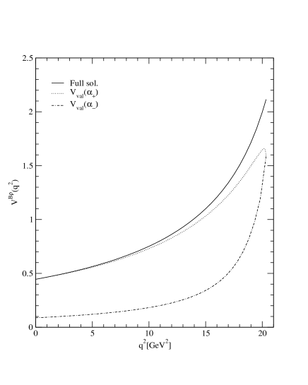
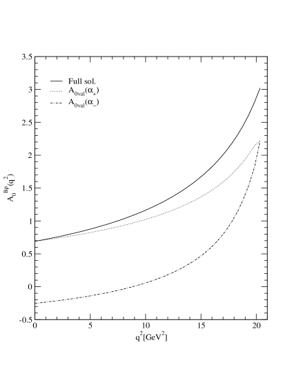
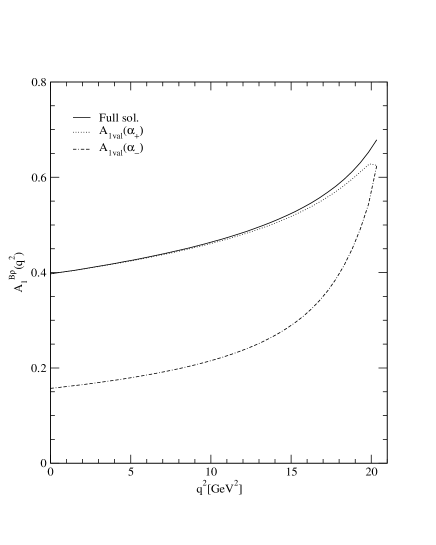
Figure 1: Weak form factors for the $B\to\rho$ transition obtained from the purely longitudinal frame. The solid, dotted, and dot-dashed lines represent the full (val + nv) solution, the valence contribution with $\alpha_{+}$-dependence, and the valence contribution with $\alpha_{-}$-dependence, respectively. The full solution is exactly identical to the covariant one.

In Fig. 1, we present the weak form factors defined in Eq. (2) for the $B\to\rho$ (heavy-to-light) transition. Since the weak form factors $V,A_{1}$, and $A_{2}$ do not involve $a_{-}$, we computed these form factors both in the $q^{+}=0$ DYW frame and in the purely longitudinal $q^{+}>0$ frame. The full results depicted by the solid lines are in complete agreement regardless of the choice of frames, as they should be. In the $q^{+}>0$ frame, we can separate the full result into the valence contribution and the nonvalence contribution. To show this, we present the valence contribution computed in the two recoil directions given by Eqs. (24) and (III.1), i.e., $\alpha_{+}$(dotted line) and $\alpha_{-}$(dot-dashed line). Note that $a_{+}$ and $a_{-}$ are obtained using both $\alpha_{+}$ and $\alpha_{-}$ solutions as shown in Eq.(III.1) and thus $A_{2}(q^{2})$ in Fig.1 doesn’t have any distinction in the valence contributions between $A_{2val}(\alpha_{+})$ and $A_{2val}(\alpha_{-})$. Of course, the nonvalence contributions are obtained by subtracting the valence contributions from the full results. We have also confirmed the agreement of the full results (solid lines) and the manifestly covariant results presented in Section II.

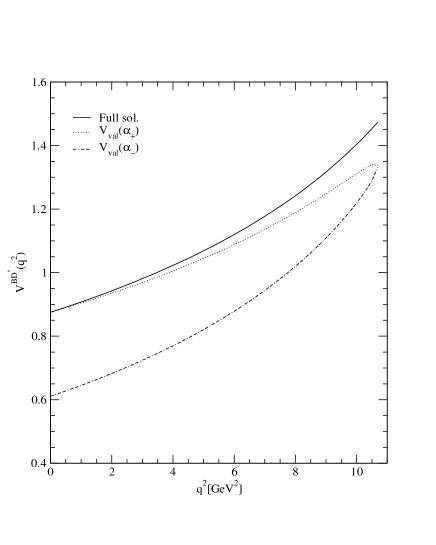
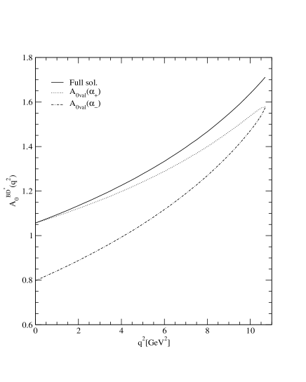
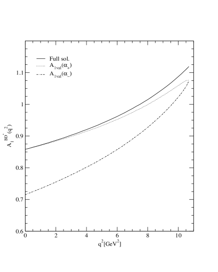
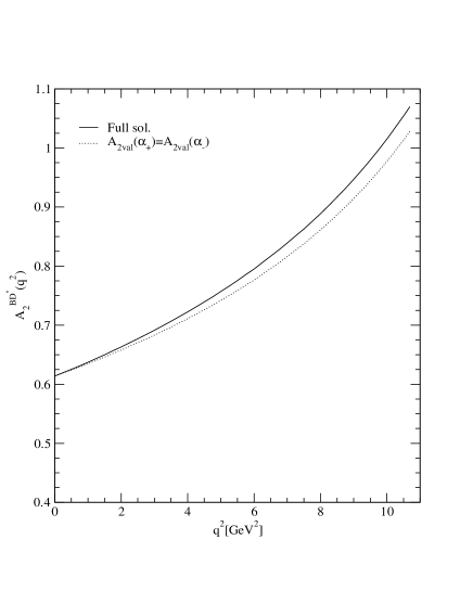
Figure 2: Weak form factors for the $B\to D^{*}$ transition obtained from the purely longitudinal frame. The solid, dotted, and dot-dashed lines represent the full (val + nv) solution, the valence contribution with $\alpha_{+}$-dependence, and the valence contribution with $\alpha_{-}$-dependence, respectively. The full solution is exactly the same as the covariant one.

In Fig. 2, we present the same for the $B\to D^{*}$ (heavy-to-heavy) transition. The general features are similar to the case of the heavy-to-light meson decay shown in Fig. 1. However, one can see that the nonvalence contributions are significantly reduced in the heavy-to-heavy case. Experimentally, two form-factor ratios for $B\to D^{*}$ decays defined by Neu ; CLEO

$$R_{1}(q^{2}) = \biggl{[}1-\frac{q^{2}}{(M_{B}+M_{D^{*}})^{2}}\biggr{]}\frac{V(q^{2})}{A_{1}(q^{2})},$$

$$R_{2}(q^{2}) = \biggl{[}1-\frac{q^{2}}{(M_{B}+M_{D^{*}})^{2}}\biggr{]}\frac{A_{2}(q^{2})}{A_{1}(q^{2})},$$ (46)

have been measured by CLEO CLEO as $R_{1}(q^{2}_{\rm max})=1.24\pm 0.26\pm 0.12$ and $R_{2}(q^{2}_{\rm max})=0.72\pm 0.18\pm 0.07$. We obtain $R_{1}(q^{2}_{\rm max})=1.05$ and $R_{2}(q^{2}_{\rm max})=0.76$, which are compatible with the these data and other theoretical predictions: $R_{1}(q^{2}_{\rm max})=1.35$ and $R_{2}(q^{2}_{\rm max})=0.79$ in Ref. Neu , $R_{1}(q^{2}_{\rm max})=1.27$ and $R_{2}(q^{2}_{\rm max})=1.01$ in Ref. ISGW2 , and $R_{1}(q^{2}_{\rm max})=1.24$ and $R_{2}(q^{2}_{\rm max})=0.91$ in Ref. AW .

The form factor $a_{-}(q^{2})$ was also constrained by the flavor independence in Ref. AW as

$$a_{+}(q^{2}_{\rm max})-a_{-}(q^{2}_{\rm max}) = -\frac{1}{\sqrt{M_{D^{*}}M_{B}}}.$$ (47)

Our value, $a_{+}-a_{-}\sim-0.36$ at $q^{2}_{\rm max}$, is consistent with Eq. (47) which yields $a_{+}-a_{-}\sim-0.31$. The form factor $a_{+}(q^{2})$ was further constrained by the flavor independence in the heavy quark limit AW and given by

$$a_{+}(q^{2}_{\rm max}) = -\frac{1}{\sqrt{4M_{D^{*}}M_{B}}}\biggl{[}1+\frac{M_{D^{*}}}{M_{B}}\biggl{(}1-\frac{M_{D^{*}}}{m_{c}}\biggr{)}\biggr{]}.$$

This yields the value $a_{+}(q^{2}_{\rm max})\sim-0.14$, which is very close to our value $a_{+}\sim-0.15$.

Table 1: The calculated $B\to\rho$ transition form factors at $q^{2}=0$.

Ref.	V	$A_{0}$	$A_{1}$	$A_{2}$
This work	0.45	0.69	0.39	0.30
LCSRBall	$0.6(2)$	–	$0.5(1)$	$0.4(2)$
LATDeb	$0.35^{+0.06}_{-0.05}$	$0.30^{+0.06}_{-0.04}$	$0.27^{+0.05}_{-0.04}$	$0.26^{+0.05}_{-0.03}$
QMJaus96	0.35	–	0.26	0.24

Table 2: The calculated $B\to D^{*}$ transition form factors at $q^{2}=0$.

Ref.	V	$A_{0}$	$A_{1}$	$A_{2}$
This work	0.89	1.07	0.87	0.62
QMJaus96	0.81	-	0.69	0.64
QMMS	0.76	0.69	0.66	0.62

Our results for the $B\to\rho$ and $B\to D^{*}$ transition form factors at $q^{2}=0$ are also compared with other theoretical results in Tables 1 and 2, respectively.

In the following subsection, we present the frame dependence of the individual valence and nonvalence contributions using the typical frames summarized in Appendix A.

IV.1 Frame dependence

We show the frame dependence of the form factors $g$ and $f$ for $B\to D^{*}$. In Figs. 3 and 4 we plotted these form factors in the Breit frame for three different orientations of the momentum transfer. The general trend we see is that the contribution to the form factor from the nonvalence diagram becomes smaller as the angle $\theta$ increases. For $\theta=\pi$, note that $q^{+}=0$ at $q^{2}=0$. Thus, the suppression of the nonvalence contribution for larger angles, close to $\theta=\pi$, is natural especially in the region near $q^{2}=0$. We found little difference between the results calculated in the Breit frame with the ones calculated in the target-rest frame, so we do not plot the latter ones.

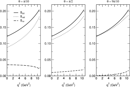
Figure 3: Breit frame $g$ form factor for $B\to D^{*}$.

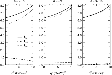
Figure 4: Breit frame $f$ form factor for $B\to D^{*}$.

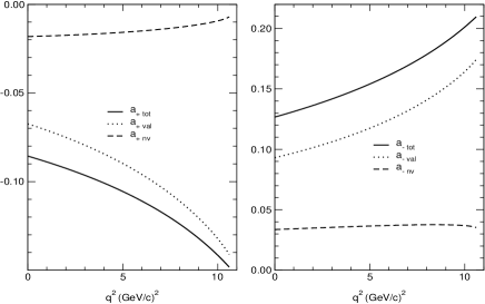
Figure 5: Breit frame $a_{\pm}$ form factors for $B\to D^{*}$.

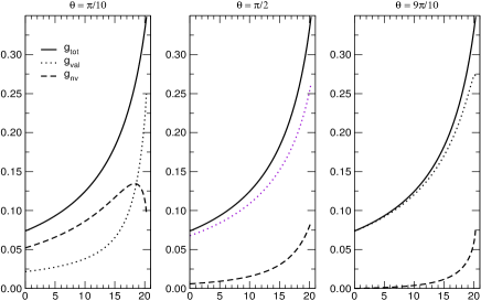
Figure 6: Breit frame $g$ form factor for $B\to\rho$.

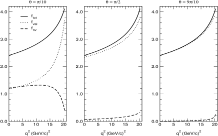
Figure 7: Breit frame $f$ form factor for $B\to\rho$.

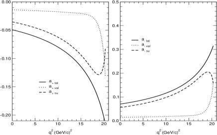
Figure 8: Breit frame $a_{\pm}$ form factors for $B\to\rho$.

We show the form factors $a_{\pm}$ in the Breit frame for $B\to D^{*}$ in Fig. 5. As explained before, we can only extract these form factors if we combine the calculations for two values of the polar angle $\theta$, i.e., two values for $\alpha$. Therefore, we do not plot the results for different values of $\theta$. In Fig.5, the used values of the polar angle are $\theta=\pi/10$ and $9\pi/10$.

The results for the heavy-to-light decay $B\to\rho$ are given in Figs. 6-8. The qualitative difference between the heavy-to-heavy and the heavy-to-light decay mentioned before is clearly seen in these figures too. The nonvalence parts become more prominent for the heavy-to-light case. In both cases the nonvalence contributions to $g$ and $f$ are suppressed for increasing polar angle $\theta$.

V Conclusion

In this work, we analyzed the transition form factors between pseudoscalar and vector mesons using both the manifestly covariant calculation and the light-front calculation for $\langle J_{V-A}^{+}\rangle$. In LFD, we presented three results: one from the DYW ($q^{+}=0$) frame, the other from the purely longitudinal $q^{+}>0$ frame, and finally results obtained in the Breit frame. In the DYW ($q^{+}=0$) frame, the transition form factors $f$,$g$, and $a_{+}$ are obtained by analytic continuation from the spacelike region. The form factor $a_{-}$ cannot be obtained in this frame unless other components of the current besides $\langle J_{V-A}^{+}\rangle$ are calculated. In the purely longitudinal $q^{+}>0$ frame, all four form factors ($f$, $g$, and $a_{\pm}$) are found from $\langle J_{V-A}^{+}\rangle$ but the nonvalence contributions should be computed in addition to the valence ones. We confirmed that all four form factors obtained in LFD are identical to the result of the manifestly covariant calculation and the DYW results for $f$, $g$, and $a_{+}$ are identical to those obtained in the purely longitudinal $q^{+}>0$ frame.

In our analysis, we do not find any zero-mode contribution to the transition form factor $f(q^{2})$ (or equivalently the axial-vector form factor $A_{1}(q^{2})$). The absence of a zero-mode is not affected by the modification of the vector meson vertex from $\Gamma^{\mu}=\gamma^{\mu}$ to $\Gamma^{\mu}_{\rm LFQM}$.

For the numerical computation, we fixed the model parameters using the normalization constraints in the elastic form factors and the available experimental data of decay constants of the pseudoscalar ($B$) and vector ($D^{*},\rho$) mesons. Comparing the results of heavy-to-light ($B\to\rho$) and heavy-to-heavy ($B\to D^{*}$) transition form factors, we find that the nonvalence contributions are significantly reduced in the heavy-to-heavy results. Our results for the $B\to D^{*}l\nu_{l}$ decay process satisfy the constraints imposed by the flavor independence on the heavy-to-heavy semileptonic decays AW .

Appendix A Kinematics

In this appendix we discuss in some detail the different reference systems we used. In our previous publicationBCJ , we used the target-rest frame (TRF), the Breit frame (BRT), and the Drell-Yan-West frame (DYW). In the present case, where the momentum transfer is timelike, the TRF is still straightforward to define, but the other frames are not. That is why we give the detailed formulas here. We write the momenta in the LFD form: $P=(P^{+},P_{x},P_{y},P^{-})$ with $P^{2}=P^{+}P^{-}-\vec{P}^{\,2}_{\bot}$.

A.1 Target-rest frame

The momentum of the inital pseudoscalar meson with mass $M_{1}$ is

$$P_{1}=\left(M_{1},0,0,M_{1}\right).{}$$ (49)

If $M_{2}$ is the mass of the vector meson, $m^{2}_{l}$ is the invariant mass square of the lepton pair in the final state, and $q$ is the four-momentum transfer, the kinematical range of $q^{2}$ is

$$m^{2}_{l}\leq q^{2}\leq(M_{1}-M_{2})^{2}.{}$$ (50)

Four-momentum conservation allows us to determine the kinematical range of the three-momentum transfer.

We write for $q$

$$q=(q^{+},\vec{q}_{\bot},q^{-}){}$$ (51)

and write

$$\vec{q}_{\bot}=Q\sin\theta\hat{n}=Q(\sin\theta\,\cos\phi,\sin\theta\,\sin\phi).{}$$ (52)

We define the quantity $M^{2}_{q}$ as follows

$$M^{2}_{q}=M^{2}_{1}-M^{2}_{2}+q^{2}{}$$ (53)

and find for the square of the length of the three-momentum transfer

$$Q^{2}=\frac{M^{4}_{q}-4M^{2}_{1}q^{2}}{4M^{2}_{1}}.{}$$ (54)

The complete expression for $q$ is

$$q=\left(\frac{M^{2}_{q}+2M_{1}Q\cos\theta}{2M_{1}},Q\sin\theta\hat{n},\frac{M^{2}_{q}-2M_{1}Q\cos\theta}{2M_{1}}\right).{}$$ (55)

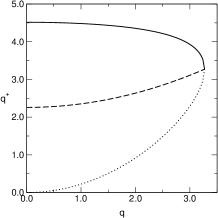
Figure 9: The quantities $q^{+}$ (top) and $\alpha=P^{+}_{2}/P^{+}_{1}$ (bottom) in the TRF for $\theta=0$ (solid), $\pi/2$ (dashed), and $\pi$ (dotted), respectively, plotted for $q=\surd q^{2}$ from 0 to $(M_{1}-M_{2})^{2}$. ($B\to D^{*}$)

The behaviour of both $q^{+}$ and $\alpha$ is smooth as can be seen in Fig. 9.

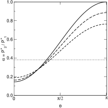
Figure 10: The quantity $\alpha=P^{+}_{2}/P^{+}_{1}$ in the TRF for $q=0$ (solid), $(M_{1}-M_{2})/2$ (long dashed), $(M_{1}-M_{2})/\surd 2$ (short dashed) and $M_{1}-M_{2}$ (dotted), respectively, plotted for $\theta$ from 0 to $\pi$. ($B\to D^{*}$)

A.2 Breit frame

The Breit frame is usually defined by the requirement that there is no energy transfer. In the case of the elastic form factors this could be achieved easily. However, for a time-like momentum $q$ the component $q^{0}$ is not allowed to vanish in the physical region. One may define a Breit-like frame in either of the two following ways.

$(i)$ Real momenta

$$P_{1}=P+q/2,\quad P_{2}=P-q/2.{}$$ (56)

For $q^{0}=0$ and $\vec{P}=0$ this choice of momenta corresponds to a particle with momentum $\vec{q}/2$ bouncing off a ‘brick wall’ and changing its momentum to $-\vec{q}/2$. This process is only possible if the particle with momentum $P_{1}$ has the same mass as the one with momentum $P_{2}$.

Our generalization drops the condition $q^{0}=0$. Then different masses, $M_{1}\neq M_{2}$, are allowed. Keeping $\vec{P}=0$ simplifies the formulas. One may relax the latter condition by a simple boost to a frame where $\vec{P}\neq 0$.

The values of $P^{0}$ and $Q=|\vec{q}|$ that correspond to the on-shell conditions $P^{2}_{1}=M^{2}_{1}$ and $P^{2}_{2}=M^{2}_{2}$ are given by

$$P^{0} = \sqrt{\frac{M^{2}_{1}+M^{2}_{2}}{2}-\frac{q^{2}}{4}},$$

$$Q = \sqrt{\frac{q^{4}-2(M^{2}_{1}+M^{2}_{2})\,q^{2}+(M^{2}_{1}-M^{2}_{2})^{2}}{2(M^{2}_{1}+M^{2}_{2})-q^{2}}}.{}$$ (57)

The LF momenta are easily obtained. As we rely on $q^{2}>0$ and real momenta, it is clear that $q^{+}>0$. We have

$$q^{+} = \sqrt{q^{2}+Q^{2}}+Q\cos\theta,$$

$$\vec{q}_{\bot} = Q\sin\theta\,\hat{n},$$

$$q^{-} = \frac{Q^{2}\sin^{2}\theta+q^{2}}{\sqrt{q^{2}+Q^{2}}+Q\cos\theta}.{}$$ (58)

Clearly, $q^{+}$ cannot vanish for real $Q$.

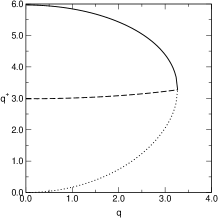
Figure 11: The quantities $q^{+}$ (upper) and $\alpha=P^{+}_{2}/P^{+}_{1}$ (lower) in the Breit frame with real momenta for $\theta=0$ (solid), $\pi/2$ (dashed), and $\pi$ (dotted), respectively, plotted for $q^{2}$ from 0 to $(M_{1}-M_{2})^{2}$. ($B\to D^{*}$)

The behaviour of both $q^{+}$ and $\alpha$ is smooth as can be seen in Fig. 11.

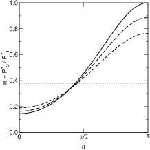
Figure 12: The quantity $\alpha=P^{+}_{2}/P^{+}_{1}$ in the Breit frame for $q=0$ (solid), $(M_{1}-M_{2})/2$ (long dashes), $(M_{1}-M_{2})/\surd 2$ (dotted) and $M_{1}-M_{2}$ (dashed), respectively, plotted for $\theta$ from 0 to $\pi$. ($B\to D^{*}$)

$(ii)$ Complex $q$
In order to avoid confusion we reserve the notation with $Q$ for the case of real momenta. In order to follow Ref. BCJ as close as possible we define

$$q=\left(q\cos\theta,i\,q\sin\theta\,\hat{n},q\cos\theta\right).{}$$ (59)

Next we determine $P$. Now we take $\vec{P}=0$, but we allow for $P^{0}\neq 0$, otherwise we shall not be able to satisfy the on-shell conditions for $P_{1}$ and $P_{2}$. Then, $P^{2}_{1}=M^{2}_{1}$ and $P^{2}_{2}=M^{2}_{2}$ give the equations

$$P^{+}+P^{-} = \frac{M^{2}_{1}-M^{2}_{2}}{q\cos\theta},$$

$$P^{+}P^{-} = \frac{M^{2}_{1}+M^{2}_{2}}{2}-\frac{q^{2}}{4}.{}$$ (60)

In the kinematically allowed domain both $P^{+}+P^{-}$ and $P^{+}P^{-}$ are positive, so both are separately positive. We find for them

$$P^{+} = \frac{M^{2}_{1}-M^{2}_{2}}{2q\cos\theta}$$

$$+\frac{1}{2}\sqrt{\frac{(M^{2}_{1}-M^{2}_{2})^{2}}{q^{2}\cos^{2}\theta}-2(M^{2}_{1}+M^{2}_{2})+q^{2}},$$

$$P^{-} = \frac{M^{2}_{1}-M^{2}_{2}}{2q\cos\theta}$$

$$-\frac{1}{2}\sqrt{\frac{(M^{2}_{1}-M^{2}_{2})^{2}}{q^{2}\cos^{2}\theta}-2(M^{2}_{1}+M^{2}_{2})+q^{2}}.$$

For this unphysical kinematics $q^{+}=0$ is allowed. The lower bound $q^{2}=0$ leads to a divergent limit for $P^{+}$, while $P^{-}$ tends to 0. Their product is of course finite for all values of $q$.

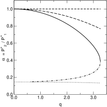
Figure 13: The quantities $q^{+}$ (upper) and $\alpha=P^{+}_{2}/P^{+}_{1}$ (lower) in the Breit frame with complex momenta for $\theta=0$ (solid), $\pi/4$ (long dashed), $\pi/2$ (short dashed), $3\pi/4$ (dotted), and $\pi$ (dot dashed), respectively, plotted for $q^{2}$ from 0 to $(M_{1}-M_{2})^{2}$. ($B\to D^{*}$)

The behaviour of $q^{+}$ is smooth (linear), but $\alpha$ has a singularity at $\theta=\pi/2$. This singularity is a branch point. For values of $\theta$ between 0 and $\pi/2$, $\alpha$ increases to 1 for all values of $q$. In the interval $[\pi/2,\pi]$ $\alpha$ increases for all $q$ from a value of $(4M^{2}_{2}-q^{2})/(4M^{2}_{1}-q^{2})$ to its value at $\theta=\pi$. This behaviour is illustrated in Fig. 14.

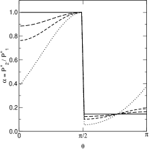
Figure 14: The quantity $\alpha=P^{+}_{2}/P^{+}_{1}$ in the Breit frame with complex momenta for $q=0$ (solid), $(M_{1}-M_{2})/2$ (long dashes), $(M_{1}-M_{2})/\surd 2$ (short dashed) and $M_{1}-M_{2}$ (dotted), respectively, plotted for $\theta$ from 0 to $\pi$. ($B\to D^{*}$)

A.3 Drell-Yan-West frame

As the DYW-frame is characterized by $q^{+}=0$, we are obliged to take $\vec{q}_{\bot}$ purely imaginary to get $q^{2}>0$. The solution of the on-shell conditions is particularly simple. Our final results are

$$q = \left(0,iq\hat{n},\frac{M^{2}_{1}-M^{2}_{2}+q^{2}}{P^{+}_{1}}\right),$$

$$P_{1} = \left(P^{+}_{1},\vec{0}_{\bot},\frac{M^{2}_{1}}{P^{+}_{1}}\right),$$

$$P_{2} = \left(P^{+}_{1},-iq\hat{n},\frac{M^{2}_{2}-q^{2}}{P^{+}_{1}}\right).{}$$ (62)

If we substitute for the arbitrary $P^{+}_{1}$ the value $M_{1}$, we obtain a quasi TRF kinematics. Needless to say that this kinematics cannot be obtained from the formulas given before for the TRF.

Appendix B Elastic form factors and decay constants of mesons with unequal quark masses

In this appendix, we summarize the manifestly covariant formulae of elastic form factors and decay constants of pseudoscalar and vector mesons with the unequal quark masses such as $B$ and $D^{*}$ mesons.

B.1 Pseudoscalar Meson Electromagnetic Form Factor

The electromagnetic form factor $F_{\rm ps}(q^{2})$ of pseudoscalar meson is defined by the matrix element given by

$$\langle P^{\prime}|J^{\mu}|P\rangle=(P^{\prime\mu}+P^{\mu})F_{\rm ps}(q^{2}),$$ (63)

where $P$ and $P^{\prime}=P+q$ are the four-momenta of initial and final states, respectively. If the meson is made of a quark and an antiquark with mass(charge) values $m_{1}(e_{1})$ and $m_{2}(e_{2})$, respectively, $F_{\rm ps}(q^{2})$ is given by

$$F_{\rm ps}(q^{2}) = \frac{g_{\rm ps}^{2}\Lambda_{1}^{4}e_{1}}{8\pi^{2}(\Lambda_{1}^{2}-m_{1}^{2})^{2}}\int_{0}^{1}dx\int_{0}^{1-x}dy\biggl{[}\{4-3(x+y)\}\ln\frac{C_{m_{2}\Lambda_{1}m_{1}}C_{m_{2}m_{1}\Lambda_{1}}}{C_{m_{2}\Lambda_{1}\Lambda_{1}}C_{m_{2}m_{1}m_{1}}}$$ (64)

$$+\{-(x+y)(x+y-1)^{2}M^{2}-(2-x-y)xyq^{2}+2(x+y-1)m_{1}m_{2}-(x+y)m_{1}^{2}\}C_{12}\biggr{]}$$

$$+(1\leftrightarrow 2),$$

where $e_{1}+e_{2}$ must be indentical to the charge of the meson,

$$C_{12}=\frac{1}{C_{m_{2}\Lambda_{1}\Lambda_{1}}}-\frac{1}{C_{m_{2}\Lambda_{1}m_{1}}}-\frac{1}{C_{m_{2}m_{1}\Lambda_{1}}}+\frac{1}{C_{m_{2}m_{1}m_{1}}}$$

(65)

and

$$C_{m_{2}\Lambda_{1}\Lambda_{1}} = (x+y)(1-x-y)M^{2}+xyq^{2}$$

$$-(x+y)\Lambda_{1}^{2}-(1-x-y)m_{2}^{2},$$

$$C_{m_{2}\Lambda_{1}m_{1}} = (x+y)(1-x-y)M^{2}+xyq^{2}$$

$$-(x\Lambda_{1}^{2}+y{m_{1}}^{2})-(1-x-y)m_{2}^{2},$$

$$C_{m_{2}m_{1}\Lambda_{1}} = (x+y)(1-x-y)M^{2}+xyq^{2}$$

$$-(x{m_{1}}^{2}+y\Lambda_{1}^{2})-(1-x-y)m_{2}^{2},$$

$$C_{m_{2}m_{1}m_{1}} = (x+y)(1-x-y)M^{2}+xyq^{2}$$ (66)

$$-(x+y){m_{1}}^{2}-(1-x-y)m_{2}^{2}.$$

B.2 Pseudoscalar Meson Decay Constant

The decay constant $f_{\rm ps}$ of a pseudoscalar meson is defined by the matrix element,

$$\langle 0|J^{\mu}_{V-A}|P\rangle=iP^{\mu}f_{\rm ps}.$$ (67)

From this definition, we find

$$f_{\rm ps} = \frac{g_{\rm ps}\Lambda_{1}^{2}\Lambda_{2}^{2}}{4\pi^{2}(\Lambda_{1}^{2}-m_{1}^{2})(\Lambda_{2}^{2}-m_{2}^{2})}\int_{0}^{1}dx$$ (68)

$$\times\{xm_{1}+(1-x)m_{2}\}\ln\frac{C_{m_{1}\Lambda_{2}}C_{\Lambda_{1}m_{2}}}{C_{\Lambda_{1}\Lambda_{2}}C_{m_{1}m_{2}}},$$

where

$$C_{m_{1}m_{2}} = x(1-x)M^{2}-xm_{1}^{2}-(1-x)m_{2}^{2},$$

$$C_{m_{1}\Lambda_{2}} = x(1-x)M^{2}-xm_{1}^{2}-(1-x)\Lambda_{2}^{2},$$

$$C_{\Lambda_{1}m_{2}} = x(1-x)M^{2}-x\Lambda_{1}^{2}-(1-x)m_{2}^{2},$$

$$C_{\Lambda_{1}\Lambda_{2}} = x(1-x)M^{2}-x\Lambda_{1}^{2}-(1-x)\Lambda_{2}^{2}.$$ (69)

B.3 Vector Meson Electromagnetic Form Factors

The electromagnetic form factors ($F_{1}(q^{2})$, $F_{2}(q^{2})$, and $F_{3}(q^{2})$) of a vector meson are defined by the matrix element between the initial state of helicity $h$ and four-momentum $P$ and the final state of $h^{\prime}$ and $P^{\prime}$:

$$\langle P^{\prime},h^{\prime}|J^{\mu}|P,h\rangle = -\epsilon^{*}_{h^{\prime}}\epsilon_{h}(P^{\prime}+P)^{\mu}F_{1}(q^{2})$$

$$+(\epsilon^{\mu}_{h}q\cdot\epsilon^{*}_{h^{\prime}}-\epsilon^{*\mu}_{h^{\prime}}q\cdot\epsilon_{h}F_{2}(q^{2})$$

$$+\frac{(\epsilon^{*}_{h^{\prime}}\cdot q)(\epsilon_{h}\cdot q)}{2M^{2}}(P^{\prime}+P)^{\mu}F_{3}(q^{2}),$$

where $\epsilon_{h}$($\epsilon^{*}_{h^{\prime}}$) is the polarization vector of the initial(final) helicity $h$($h^{\prime}$) state. If the meson is made of a quark and an antiquark with mass(charge) values $m_{1}(e_{1})$ and $m_{2}(e_{2})$, respectively, $F_{i}(q^{2})$($i=1,2,3$) are given by

$$F_{1}(q^{2}) = \frac{g_{\rm v}^{2}\Lambda_{1}^{4}e_{1}}{8\pi^{2}(\Lambda_{1}^{2}-m_{1}^{2})^{2}}\int_{0}^{1}dx\int_{0}^{1-x}dy\biggl{[}(2-x-y)\ln\frac{C_{m_{2}\Lambda_{1}m_{1}}C_{m_{2}m_{1}\Lambda_{1}}}{C_{m_{2}\Lambda_{1}\Lambda_{1}}C_{m_{2}m_{1}m_{1}}}$$ (71)

$$+\{-(x+y)(x+y-1)^{2}M^{2}-(2-x-y)xyq^{2}+2(x+y-1)m_{1}m_{2}-(x+y)m_{1}^{2}\}C_{12}\biggr{]}$$

$$+(1\leftrightarrow 2),$$

$$F_{2}(q^{2}) = -\frac{g_{\rm v}^{2}\Lambda_{1}^{4}e_{1}}{8\pi^{2}(\Lambda_{1}^{2}-m_{1}^{2})^{2}}\int_{0}^{1}dx\int_{0}^{1-x}dy\biggl{[}(2+x+y)\ln\frac{C_{m_{2}\Lambda_{1}m_{1}}C_{m_{2}m_{1}\Lambda_{1}}}{C_{m_{2}\Lambda_{1}\Lambda_{1}}C_{m_{2}m_{1}m_{1}}}$$ (72)

$$+\{(x+y)(x+y+1)(x+y-1)M^{2}-xy(x+y)q^{2}-(x+y){m_{1}}^{2}-2m_{1}m_{2}\}C_{12}\biggr{]}$$

$$+ (1\leftrightarrow 2),$$

$$F_{3}(q^{2}) = \frac{g_{\rm v}^{2}\Lambda_{1}^{4}e_{1}}{8\pi^{2}(\Lambda_{1}^{2}-m_{1}^{2})^{2}}\int_{0}^{1}dx\int_{0}^{1-x}dy\;8xy(x+y-1)M^{2}C_{12}+(1\leftrightarrow 2),$$ (73)

where $e_{1}+e_{2}$ must be equal to the charge of the meson and $C_{12}$ is identical to the one given in Eq. (65).

B.4 Vector Meson Decay Constant

The decay constant $f_{\rm v}$ of a vector meson is defined by the matrix element,

$$\langle 0|J^{\mu}_{V-A}|P,h\rangle=iMf_{\rm v}\epsilon^{\mu}(h),$$ (74)

where $\epsilon(h)$ is the polarization vector of helicity $h$ state. From this definition, we find

$$f_{\rm v} = \frac{g_{\rm v}\Lambda_{1}^{2}\Lambda_{2}^{2}}{4\pi^{2}M(\Lambda_{1}^{2}-m_{1}^{2})(\Lambda_{2}^{2}-m_{2}^{2})}\int_{0}^{1}dx$$

$$\times\biggl{[}\{m_{1}m_{2}+x(1-x)M^{2}\}\ln\frac{C_{m_{1}\Lambda_{2}}C_{\Lambda_{1}m_{2}}}{C_{\Lambda_{1}\Lambda_{2}}C_{m_{1}m_{2}}}$$

$$- C_{\Lambda_{1}\Lambda_{2}}\ln(-C_{\Lambda_{1}\Lambda_{2}})+C_{m_{1}\Lambda_{2}}\ln(-C_{m_{1}\Lambda_{2}})$$

$$+ C_{\Lambda_{1}m_{2}}\ln(-C_{\Lambda_{1}m_{2}})-C_{m_{1}m_{2}}\ln(-C_{m_{1}m_{2}})\biggr{]},$$

where $C_{m_{1}m_{2}}$, $C_{m_{1}\Lambda_{2}}$, $C_{\Lambda_{1}m_{2}}$, $C_{\Lambda_{1}\Lambda_{2}}$ are given by Eq. (B.2).

Appendix C Analytic expressions of $g(q^{2})$, $a_{+}(q^{2})$, and $f(q^{2})$ in the $q^{+}=0$ frame for $\Gamma^{+}=\gamma^{+}$

For the numerical analysis of the weak form factors in the $q^{+}=0$ frame, we use Feynman parameterization to integrate out the transverse momentum, ${\bf k}_{\perp}$.

Similar to the covariant analysis, we first separate the energy denominators as follows:

$$\frac{1}{(M^{2}_{1}-M^{2}_{0})(M^{2}_{1}-M^{2}_{\Lambda_{1}})(M^{2}_{2}-M^{\prime 2}_{0})(M^{2}_{2}-M^{\prime 2}_{\Lambda_{2}})}$$

$$=\frac{(1-x)^{2}}{(m^{2}_{1}-\Lambda^{2}_{1})(m^{2}_{2}-\Lambda^{2}_{2})}\biggl{(}\frac{1}{N_{1}}-\frac{1}{N_{1\Lambda}}\biggr{)}\biggl{(}\frac{1}{N_{2}}-\frac{1}{N_{2\Lambda}}\biggr{)}$$

where $N_{1}=M^{2}_{1}-M^{2}_{0}$, $N_{1\Lambda}=M^{2}_{1}-M^{2}_{\Lambda_{1}}$, $N_{2}=M^{2}_{2}-M^{\prime 2}_{0}$, and $N_{2\Lambda}=M^{2}_{2}-M^{\prime 2}_{\Lambda_{2}}$.

Now using Feynman parametrization

$${}\frac{1}{ab} = \int^{1}_{0}\frac{dx}{[ax+b(1-x)]^{2}}$$ (77)

we obtain from Eqs. (31), (32), and (37)

$${}g(q^{2}) = \frac{{\cal N}}{8\pi^{2}}\int^{1}_{0}xdx\int^{1}_{0}dy\biggl{[}{\cal A}_{p}-x(1-y)(m_{1}-m_{2})\biggr{]}$$ (78)

$$\times\biggl{\{}\frac{1}{a_{1}y+a_{2}(1-y)+y(1-y)x^{2}q^{2}}-(a_{2}\to a_{2\Lambda})-(a_{1}\to a_{1\Lambda})+(a_{1}\to a_{1\Lambda},a_{2}\to a_{2\Lambda})\biggr{\}},$$

$$a_{+}(q^{2}) = \frac{{\cal N}}{8\pi^{2}}\int^{1}_{0}xdx\int^{1}_{0}dy\biggl{[}(1-2x){\cal A}_{p}-x(1-y)[(1-2x)m_{1}-m_{2}-2(1-x)m]\biggr{]}$$ (79)

$$\times\biggl{\{}\frac{1}{a_{1}y+a_{2}(1-y)+y(1-y)x^{2}q^{2}}-(a_{2}\to a_{2\Lambda})-(a_{1}\to a_{1\Lambda})+(a_{1}\to a_{1\Lambda},a_{2}\to a_{2\Lambda})\biggr{\}},$$

$$f(q^{2}) = (M^{2}_{1}-M^{2}_{2}-q^{2})a_{+}(q^{2})-\frac{{\cal N}}{4\pi^{2}}\int^{1}_{0}dx\int^{1}_{0}dy\biggl{\{}C_{1}\biggl{[}\frac{1}{a_{1}y+a_{2}(1-y)+y(1-y)x^{2}q^{2}}-(a_{2}\to a_{2\Lambda})$$ (80)

$$\hskip 56.9055pt-(a_{1}\to a_{1\Lambda})+(a_{1}\to a_{1\Lambda},a_{2}\to a_{2\Lambda})\biggr{]}-C_{2}\ln\biggl{(}\frac{a_{12\Lambda}a_{1\Lambda 2}}{a_{12}a_{1\Lambda 2\Lambda}}\biggr{)}\biggr{\}}$$

where

$${}a_{1} = x(1-x)M^{2}_{1}-xm^{2}_{1}-(1-x)m^{2}$$

$$a_{2} = x(1-x)M^{2}_{2}-xm^{2}_{2}-(1-x)m^{2}$$

$$a_{1\Lambda} = a_{1}(m_{1}\to\Lambda_{1}),a_{2\Lambda}=a_{2}(m_{2}\to\Lambda_{2}),$$ (81)

$${}C_{1} = {\cal A}_{p}[x(1-x)M^{2}_{2}+m_{2}m-x^{2}q^{2}]$$

$$-x^{2}(1-y)^{2}(xm_{1}+m_{2}-xm)q^{2}$$

$$+x^{2}(1-y)[2x(m_{1}-m)+m_{2}+m]q^{2}$$

$$C_{2} = x(m_{1}-m)+m_{2},$$ (82)

and

$${}a_{12} = a_{1}y+a_{2}(1-y)+y(1-y)x^{2}q^{2}$$

$$a_{12\Lambda} = a_{1}y+a_{2\Lambda}(1-y)+y(1-y)x^{2}q^{2}$$

$$a_{1\Lambda 2} = a_{1\Lambda}y+a_{2}(1-y)+y(1-y)x^{2}q^{2}$$

$$a_{1\Lambda 2\Lambda} = a_{1\Lambda}y+a_{2\Lambda}(1-y)+y(1-y)x^{2}q^{2}$$ (83)

Appendix D Form factors $g(q^{2})$, $a_{+}(q^{2})$, and $f(q^{2})$ in the $q^{+}=0$ frame for $\Gamma^{+}_{\rm LFQM}$

In this appendix, we give the exact LF expressions for the form factors $g(q^{2}),a_{+}(q^{2})$, and $f(q^{2})$ in the $q^{+}=0$ frame for the more realistic LF vector meson vertex function given by Eq. (41). We shall write $g^{\rm LFQM}(q^{2})$, $a^{\rm LFQM}_{+}(q^{2})$, and $f^{\rm LFQM}(q^{2})$ for the vertex $\Gamma^{+}_{\rm LFQM}$ to distinguish them from those obtained for $\Gamma^{+}=\gamma^{+}$.

To obtain the form factor $g(q^{2})$, we first calculate the trace $T^{+(h=1)}_{V}$ for the vector current with transverse polarization, which is given by

$$T^{+(h=1)}_{V} = -4i\frac{(p_{2}-k)\cdot\epsilon^{*}(h=1)}{M^{\prime}_{0}+m_{2}+m}$$

$$\;\;\times\epsilon^{+\mu\nu\sigma}(p_{1\rm on})_{\mu}(p_{2\rm on})_{\nu}(k_{\rm on})_{\sigma}$$

$$= -4\sqrt{2}P^{+}_{1}\epsilon^{+-xy}\frac{{\bf k}^{2}_{\perp}q^{L}-({\bf k}_{\perp}\cdot{\bf q}_{\perp})k^{L}}{M^{\prime}_{0}+m_{2}+m},$$

where we use the identity $({\bf k}_{\perp}\times{\bf q}_{\perp})_{z}=i(k^{R}q^{L}-{\bf k}_{\perp}\cdot{\bf q}_{\perp})$. Note that $T^{+(h=1)}_{V}$ is independent of $k^{-}$ (which is due to $\epsilon^{+}(h=1)=0$) and thus free from the zero-mode contribution as in the case of $\Gamma^{+}=\gamma^{+}$.

Modifying $S^{+(h=1)}_{{\rm on}\;V}\to S^{+(h=1)}_{{\rm on}\;V}-T^{+(h=1)}_{V}$ in Eq. (III) for $\Gamma^{+}$ given by Eq. (41), we obtain the form factor $g^{\rm LFQM}(q^{2})$ in the $q^{+}=0$ frame as

$${}g^{\rm LFQM}(q^{2}) = -\frac{g_{1}g_{2}\Lambda^{2}_{1}\Lambda^{2}_{2}}{(2\pi)^{3}}\int^{1}_{0}\frac{dx}{x(1-x)^{4}}\int d^{2}{\bf k}_{\perp}\frac{1}{(M^{2}_{1}-M^{2}_{0})(M^{2}_{1}-M^{2}_{\Lambda_{1}})(M^{2}_{2}-M^{\prime 2}_{0})(M^{2}_{2}-M^{\prime 2}_{\Lambda_{2}})}$$ (85)

$$\times\biggl{\{}{\cal A}_{P}+\frac{{\bf k}_{\perp}\cdot{\bf q}_{\perp}}{{\bf q}^{2}_{\perp}}(m_{1}-m_{2})+\frac{2}{M^{\prime}_{0}+m_{2}+m}\biggl{[}{\bf k}^{2}_{\perp}-\frac{({\bf k}_{\perp}\cdot{\bf q}_{\perp})^{2}}{{\bf q}^{2}_{\perp}}\biggr{]}\biggr{\}}.$$

We note that our result for $g^{\rm LFQM}(q^{2})$ in Eq. (85) is equivalent to that obtained by Jaus Jaus (see, for example, Eq. (4.13) in Ref. Jaus ) and free from the zero-mode contribution.

Now, the trace $T^{+(h)}_{A}$ for the axial-vector current is given by

$$T^{+(h)}_{A} = 4\frac{(p_{2}-k)\cdot\epsilon^{*}(h)}{M^{\prime}_{0}+m_{2}+m}\biggl{[}(p_{2\rm on}\cdot k_{\rm on}-m_{2}m)p^{+}_{1}$$ (86)

$$+ (p_{1\rm on}\cdot k_{\rm on}+m_{1}m)p^{+}_{2}-(p_{1\rm on}\cdot p_{2\rm on}+m_{1}m_{2})k^{+}$$

$$+ (k^{-}-k^{-}_{\rm on})p^{+}_{1}p^{+}_{2}\biggr{]}.$$

The form factor $a_{+}^{\rm LFQM}(q^{2})$ in the $q^{+}=0$ frame is obtained from the axial-vector current with transverse polarization ($h=1$) (see the $\alpha\to 1$ limit in Eq. (III)). Explicitly, the trace is given by

$$T^{+(h=1)}_{A} = -\frac{4\sqrt{2}P^{+}_{1}}{x(M^{\prime}_{0}+m_{2}+m)}(xq^{L}+k^{L})$$ (87)

$$\times \biggl{\{}{\bf k}_{\perp}\cdot{\bf k^{\prime}}_{\perp}+[(1-x)m-xm_{2}]{\cal A}_{p}$$

$$\;\;+\;x(1-x)^{2}(k^{-}-k^{-}_{\rm on})P^{+}_{1}\biggr{\}}.$$

Even though $(p_{2}-k)\cdot\epsilon^{*}(h=1)$ is independent of $k^{-}$, there is a possibility to get a zero-mode contribution from the last term, i.e., the term proportional to $(k^{-}-k^{-}_{\rm on})$, in Eq. (86) or  (87). While the valence part, $[T^{+(h=1)}_{A}]_{\rm val}$, is obtained for $k^{-}=k^{-}_{\rm on}$, the zero-mode part, $[T^{+(h=1)}_{A}]_{\rm zm}$, is obtained for $k^{-}=k^{-}_{m_{1}}$ or $k^{-}=k^{-}_{\Lambda_{1}}$. However, counting only the longitudinal momentum fraction terms, one can easily find from Eq. (87) that the zero-mode part of $T^{+(h=1)}_{A}$ vanishes as $[T^{+(h=1)}_{A}]_{zm}\sim(1-x)^{3/2}$ in the $\alpha\to 1$ (or $x\to 1$) limit and the valence part as $\sim\sqrt{1-x}$ in the $x\to 1$ limit. Therefore, following the argument given in Sec. III.4, there is no zero-mode contribution to the form factor $a^{\rm LFQM}_{+}(q^{2})$. Modifying $S^{+(h=1)}_{{\rm on}\;A}\to S^{+(h=1)}_{{\rm on}\;A}-[T^{+(h=1)}_{A}]_{\rm val}$ in Eq. (III) and taking the limit of $\alpha\to 1$, we obtain

$${}a^{\rm LFQM}_{+}(q^{2}) = -\frac{g_{1}g_{2}\Lambda^{2}_{1}\Lambda^{2}_{2}}{(2\pi)^{3}}\int^{1}_{0}\frac{dx}{x(1-x)^{4}}\int d^{2}{\bf k}_{\perp}\frac{1}{(M^{2}_{1}-M^{2}_{0})(M^{2}_{1}-M^{2}_{\Lambda_{1}})(M^{2}_{2}-M^{\prime 2}_{0})(M^{2}_{2}-M^{\prime 2}_{\Lambda_{2}})}$$ (88)

$$\times\biggl{\{}(1-2x){\cal A}_{P}+\frac{{\bf k}_{\perp}\cdot{\bf q}_{\perp}}{{\bf q}^{2}_{\perp}}\;[\;(1-2x)m_{1}-m_{2}-2(1-x)m\;]$$

$$\hskip 14.22636pt-\frac{2(x{\bf q}^{2}_{\perp}+{\bf k}_{\perp}\cdot{\bf q}_{\perp})}{x{\bf q}^{2}_{\perp}(M^{\prime}_{0}+m_{2}+m)}[{\bf k}_{\perp}\cdot{\bf k^{\prime}}_{\perp}+((1-x)m-xm_{2}){\cal A}_{P}]\biggr{\}},$$

which is again equivalent to that obtained by Jaus Jaus (see, for example, his Eq. (4.14)).

Finally, we need to compute the trace in Eq. (86) with the longitudinal polarization vector ($h=0$) to obtain $f^{\rm LFQM}(q^{2})$. Here we again separate the trace term, $T^{+(h=0)}_{A}$, into the valence part, $[T^{+(h=0)}_{A}]_{\rm val}$, with $k^{-}=k^{-}_{\rm on}$ and the possible zero-mode part, $[T^{+(h=0)}_{A}]_{\rm zm}$, with $k^{-}=k^{-}_{m_{1}}$ and $k^{-}=k^{-}_{\Lambda_{1}}$. Explicitly, the valence part is given by

$$[T^{+(h=0)}_{A}]_{\rm val} = -\frac{4P^{+}_{1}}{xM_{2}(M^{\prime}_{0}+m_{2}+m)}$$

$$\times \{xM^{2}_{2}+(1-x)M^{\prime 2}_{0}\}$$

$$\times \{{\bf k}_{\perp}\cdot{\bf k^{\prime}}_{\perp}+[(1-x)m-xm_{2}]{\cal A}_{P}\},$$

while the possible zero-mode part for $k^{-}=k^{-}_{\Lambda_{1}}$ is given by

$$[T^{+(h=0)}_{A}]_{\rm zm} = \frac{4P^{+}_{1}}{xM_{2}(M^{\prime}_{0}+m_{2}+m)}$$ (90)

$$\times \{x{\tilde{M}}^{2}_{\Lambda_{1}}+xM^{2}_{2}-M^{2}_{1}-{\bf q}^{2}_{\perp}\}$$

$$\times \{{\bf k}_{\perp}\cdot{\bf k^{\prime}}_{\perp}+[(1-x)m-xm_{2}]{\cal A}_{P}$$

$$+x(1-x)^{2}(M^{2}_{1}-M^{2}_{\Lambda_{1}})\},$$

where ${\tilde{M}}^{2}_{\Lambda_{1}}$ is defined as

$${\tilde{M}}^{2}_{\Lambda_{1}}=\frac{\Lambda^{2}_{1}+[{\bf k}_{\perp}-(1-x){\bf q}^{2}_{\perp}]}{x(1-x)}.$$ (91)

The zero-mode part for $k^{-}=k^{-}_{m_{1}}$ can be easily obtained by changing $\Lambda_{1}\to m_{1}$ in Eq. (90).

Counting the longitudinal momentum fraction terms in Eq. (90), one can easily find the singular behavior given by Eq.(44), i.e.

$$[T^{+(h=0)}_{A}]_{\rm zm}\sim\sqrt{\frac{1}{1-x}}$$ (92)

as $x\to 1$. However, as we showed in Sec. III.5 (see Eq.(45)), there is no zero-mode contribution to $f^{\rm LFQM}(q^{2})$ even though the trace term itself shows singular behavior as $x\to 1$.

Therefore, the form factor $f^{\rm LFQM}(q^{2})$ in the $q^{+}=0$ frame can be obtained from the valence contribution only (see Eq. (III)) and it is given by

$$f^{\rm LFQM}(q^{2})=\frac{M_{2}}{P^{+}_{1}}\langle J^{+}_{A}\rangle^{h=0}_{\rm LFQM}-(M^{2}_{1}-M^{2}_{2}+{\bf q}^{2}_{\perp})a^{\rm LFQM}_{+}(q^{2}),$$ (93)

where

$${}\langle J^{+}_{A}\rangle^{h=0}_{\rm LFQM} = \frac{g_{1}g_{2}\Lambda^{2}_{1}\Lambda^{2}_{2}}{(2\pi)^{3}}\int^{1}_{0}\frac{dx}{x(1-x)^{4}}\int d^{2}{\bf k}_{\perp}\frac{S^{+(h=0)}_{\rm on\;A}-[T^{+(h=0)}_{A}]_{\rm val}}{(M^{2}_{1}-M^{2}_{0})(M^{2}_{1}-M^{2}_{\Lambda_{1}})(M^{2}_{2}-M^{\prime 2}_{0})(M^{2}_{2}-M^{\prime 2}_{\Lambda_{2}})}.$$ (94)

We note the difference from the conclusion drawn by Jaus Jaus ; Jaus02 , where the author claimed that the form factor $f(q^{2})$ receives a zero-mode contribution.

References

(1) B. L. G. Bakker, H.-M. Choi, and C.-R. Ji,
Phys. Rev. D 65, 116001 (2002).
(2) S.-J. Chang and T.-M. Yan, Phys. Rev. D 7, 1147 (1973);
7, 1780 (1973); M. Burkardt, Nucl. Phys. A 504, 762 (1989);
S. J. Brodsky and D. S. Hwang, Nucl. Phys. B 543, 239 (1998);
N.C.J. Schoonderwoerd and B.L.G. Bakker, Phys. Rev. D 57, 4965 (1998);
H.-M. Choi and C.-R. Ji, Phys. Rev. D 58, 071901 (1998);
J.P.B.C. de Melo et al.,Nucl. Phys. A 631, 574c (1998).
(3) B. L. G. Bakker and C.-R. Ji,
Phys. Rev. D 65, 073002 (2002).
(4) I.L. Grach and L.A. Kondratyuk,
Sov. J. Nucl. Phys. 39, 198 (1984).
(5) S.J. Brodsky and J.R. Hiller,
Phys. Rev. D 46, 2141 (1992).
(6) P.L. Chung, F. Coester, B.D. Keister
and W. N. Polyzou, Phys. Rev. C 37, 2000 (1988).
(7) C.-R.Ji and H.-M.Choi, Nucl. Phys. Proc. Suppl. 90, 93 (2000).
(8) W. Jaus, Phys. Rev. D 41, 3394 (1990).
(9) W. Jaus, Phys. Rev. D 53, 1349 (1996).
(10) D. Melikhov and B. Stech, Phys. Rev. D 62, 014006 (2000).