Three Loop Top Quark Contributions
to the $\rho$ Parameter

Abstract

We present results for the three-loop top quark contributions to the $\rho$ parameter in the limit of large top quark mass. The simultaneous dependence on the mass of the Higgs boson $M_{H}$ and the mass of the top quark $m_{t}$ is obtained from expansions in the range of $M_{H}$ around $m_{t}$ and in the limit $M_{H}\gg m_{t}$. In combination with the previous result for $M_{H}=0$ the dependence of the $\rho$ parameter on the leading Yukawa contributions, i.e. on $m_{t}$ and $M_{H}$, is well under control for all mass values of practical importance. The effects lead to a shift in the $W$ mass in the order of 5 MeV and are relevant for precision measurements at TESLA.

1 Introduction

The standard model predicts a strong influence of virtual heavy top quarks in the low energy limit on four-fermion processes through their virtual contributions to the W and Z boson self energies [1]. This effect allows the indirect determination of the mass of the Higgs boson and is generally essential for electroweak precision tests.

The bulk of the heavy top quark corrections to the W and Z self energies can be collected in a deviation of the so called $\rho$ parameter from the tree level result $\rho_{\mbox{\small tree}}=1$. The $\rho$ parameter is usually defined by the ratio of the neutral and charged current coupling constants at zero momentum transfer [1]:

$$\rho=\frac{J_{NC}(0)}{J_{CC}(0)}\,,$$ (1)

where $J_{CC}(0)$ is given by the Fermi coupling constant $G_{F}$ determined from the $\mu$-decay rate whereas $J_{NC}(0)$ is measured by neutrino scattering on electrons or hadrons.

In leading order contributions from the Yukawa coupling of the top quark to $\rho$ are parameterized in terms of $\Delta\rho$. This contributions stem from the transversal parts of the self energies of the $W$- and $Z$-boson:

$$\rho=\frac{1}{1-\Delta\rho}\approx\frac{1}{c^{2}}\,\frac{M_{W}^{2}-\Pi_{T}^{WW}(0)}{M_{Z}^{2}-\Pi_{T}^{ZZ}(0)},$$ (2)

where $c^{2}=M_{W}^{2}/M_{Z}^{2}$ represents the cosine of the weak mixing angle, defined in the standard on-shell scheme. Corrections from vertex and box diagrams always involve extra powers of the weak coupling constant $g_{weak}^{2}$ and are thus suppressed by powers of $(g_{\rm weak}/g_{\rm Yukawa}^{\rm top})^{2}$, i.e. $(M_{W}/m_{t})^{2}$.

In this context $\Pi_{T}^{WW}(0)$ and $\Pi_{T}^{ZZ}(0)$ can be taken as the bare one-particle irreducible amplitudes. The divergencies are absorbed by the Higgs mass, top mass, and W boson mass renormalization, i.e. by expressing the bare $m_{t}$, $M_{H}$, and $M_{W}$ in terms of the renormalized quantities. In the following we will first express the final answer in terms of the $\overline{\mbox{MS}}$ top mass $m_{t}$, the on-shell Higgs mass $M_{H}$, and the low energy Fermi constant $G_{F}$ obtained from $\mu$-decay. The latter is introduced to absorb the vector boson mass $M_{W}$. In a last step the transformation from the $\overline{\mbox{MS}}$ top quark mass $m_{t}$ to the on-shell top quark mass $M_{t}$ will be performed.

The first two-loop results for $\Delta\rho$ in the limits $M_{H}\rightarrow 0$ and $M_{H}\gg m_{t}$ for large $m_{t}$ can be found in [2], for arbitrary $M_{H}$ in [3]. The result for $\Delta\rho$ of order $G_{F}m_{t}^{2}\alpha_{s}^{2}$ was obtained in [4]. By including terms of $\mathcal{O}(M_{W}^{2}/m_{t}^{2})$ this has even been extended to predictions for $\Delta r$ in three-loop approximation.

The present paper is concerned with mixed QCD and electroweak contributions of order $(G_{F}m_{t}^{2})^{2}\alpha_{s}$ and purely electroweak contributions of order $(G_{F}m_{t}^{2})^{3}$. It extends the result of [5] where the special case $M_{H}=0$ has been considered. Using the technique of heavy mass expansion for the limit $M_{H}\gg m_{t}$ and considering sufficiently many terms leads to stable predictions down to Higgs Mass values as low as twice $m_{t}$. $\Delta\rho$ is furthermore evaluated for $M_{H}$ around $m_{t}$, and with the help of expansions, a stable approximation is provided in the region from close to zero up to twice $m_{t}$. Combining the results from the different regions, the three-loop corrections to the $\rho$ parameter are well under control.

An outline of the calculation, including a short discussion of the renormalization, is given in section 2. In section 4 the transformation of the top quark mass from the $\overline{\mbox{MS}}$ scheme to the on-shell top mass is treated in detail. Our results at order $G_{F}^{3}$ and $\alpha_{s}G_{F}^{2}$ are presented in sections 3 and 5 in the $\overline{\mbox{MS}}$ and on-shell definition for the top quark mass respectively.

2 Treatment of diagrams and renormalization

The computation of the three-loop contributions to $\Delta\rho$ at orders $G_{F}^{3}$ and $\alpha_{s}G_{F}^{2}$ for $M_{H}\approx m_{t}$ and $M_{H}\gg m_{t}$ is similar to the one discussed in [5] for $M_{H}=0$. The same Feynman diagrams contribute: $W$ and $Z$ boson self energies up to three loops, top quark self energies up to two loops, one-loop Higgs boson self energies, and Higgs tadpoles up to two loops. All diagrams were generated using the program QGRAF [6].

In comparison to [5] a non-vanishing Higgs mass introduces a second mass scale into the problem. In order to calculate such diagrams we consider two different ranges of the Higgs mass: First, in the range of $M_{H}$ around $m_{t}$ we perform a straightforward Taylor expansion in the mass difference $M_{H}-m_{t}$ around the point $M_{H}=m_{t}$. In the second region, i.e. for $M_{H}\gg m_{t}$, we use asymptotic expansions [7] and made use of the program EXP [8]. In both cases the resulting diagrams contained at most one non-vanishing mass scale.

From equation (2) the vector boson self energies can be taken at zero external momentum. After the application of the expansion procedures the resulting integrals are of tadpole type with one mass scale. Their computation can be performed using the program package MATAD [9] written in FORM [10]. Apparently the Higgs tadpoles, which are needed to renormalize the vacuum expectation value of the Higgs boson, can be treated using the same program package. To renormalize the mass of the Higgs boson, the computation of on-shell Higgs boson self energy diagrams is necessary. The corresponding renormalization constant is needed to one-loop order only and the relevant integrals are straightforward. The remaining two-loop top quark mass renormalization is, however, more involved, in particular in the on-shell scheme. Details on this issue are given in sections 3 and 4.

The whole calculation was performed using dimensional regularization and anticommuting $\gamma_{5}$. This prescription preserves the Ward–Takahashi identities which relate the self energies of the gauge bosons to the non-diagonal self energies of the gauge-to-goldstone and the goldstone boson self energies. The validity of these identities was verified by explicit calculations.

3 The $\rho$-parameter in the $\overline{\mbox{MS}}$ scheme

In this section we present our results for the $\overline{\mbox{MS}}$ definition of the top quark mass. The renormalization constant of the top quark mass can be obtained by calculating the relevant one- and two-loop self energy diagrams in the limit of vanishing external momentum. After the application of the expansions mentioned in section 2, the remaining integrals were computed using the program package MATAD.

The radiative corrections to $\Delta\rho$ depend on the $\overline{\mbox{MS}}$ top mass $m_{t}\equiv m_{t}(m_{t})$, the on-shell Higgs mass $M_{H}$, the Fermi constant $G_{F}$ and the strong coupling constant $\alpha_{s}$ and are written as follows:

$$\Delta\rho = x_{t}\,\Delta\rho^{(x_{t})}+x_{t}^{2}\,\Delta\rho^{(x_{t}^{2})}+\frac{\alpha_{s}}{\pi}\,x_{t}\,\Delta\rho^{(\alpha_{s}x_{t})}+\left(\frac{\alpha_{s}}{\pi}\right)^{2}x_{t}\,\Delta\rho^{(\alpha_{s}^{2}x_{t})}$$ (3)

$$\mbox{}+\frac{\alpha_{s}}{\pi}\,x_{t}^{2}\,\Delta\rho^{(\alpha_{s}x_{t}^{2})}+x_{t}^{3}\,\Delta\rho^{(x_{t}^{3})}+\cdots\,,$$

with

$$x_{t}=\frac{G_{F}m_{t}^{2}}{8\sqrt{2}\pi^{2}}\approx 3.0\cdot 10^{-3}\,.$$

Here and later on we always set the $\overline{\mbox{MS}}$ renormalization scale $\mu$ equal to $m_{t}$

In this paper we evaluate the coefficients $\Delta\rho^{(x_{t}^{3})}$ and $\Delta\rho^{(\alpha_{s}x_{t}^{2})}$. Numerically they are given by:

$M_{H}=0$:

$$\Delta\rho^{(x_{t}^{3})} = 47.73\ ,$$ (4)

$$\Delta\rho^{(\alpha_{s}x_{t}^{2})} = 76.91\ .$$ (5)

$M_{H}\approx m_{t}$: In this case we have computed five terms in the expansion in $\delta$ defined by the relation $M_{H}=m_{t}(1+\delta)$:

$$\Delta\rho^{(x_{t}^{3})} = -40.30-138.26\,\delta-32.39\,\delta^{2}+10.32\,\delta^{3}-3.27\,\delta^{4}-0.01\,\delta^{5}+\mathcal{O}(\delta^{6})\,,$$ (6)

$$\Delta\rho^{(\alpha_{s}x_{t}^{2})} = 93.07+21.27\,\delta+0.53\,\delta^{2}-2.29\,\delta^{3}+1.14\,\delta^{4}-0.51\,\delta^{5}+\mathcal{O}(\delta^{6})\,.$$ (7)

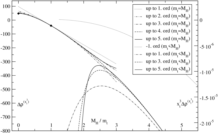
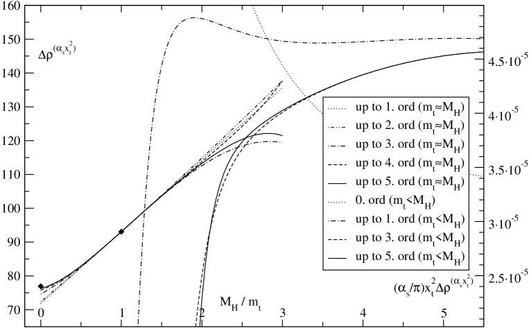
Figure 1: Contributions of order $x_{t}^{3}$ to $\Delta\rho$ in the $\overline{\mbox{MS}}$ definition of the top quark mass. The black squares indicate the points where the exact result is known.

Figure 2: Contributions of order $\alpha_{s}x_{t}^{2}$ to $\Delta\rho$ in the $\overline{\mbox{MS}}$ definition of the top quark mass. The black squares indicate the points where the exact result is known.

$M_{H}\gg m_{t}$: The application of the hard mass procedure leads to an expansion in the ratio $y\equiv 4m_{t}^{2}/M_{H}^{2}$:

$$\Delta\rho^{(x_{t}^{3})} = \frac{1}{y}(-12.80+24.75\,\log y)$$

$$- 192.86-394.05\,\log y-275.02\,\log^{2}y-24.25\,\log^{3}y$$

$$+ y\,\left(-337.88+408.59\,\log y-233.35\,\log^{2}y+108.04\,\log^{3}y\right)$$

$$+ y^{2}\,\left(82.56-378.31\,\log y+26.14\,\log^{2}y+48.60\,\log^{3}y\right)$$

$$+ y^{3}\,\left(-82.58-291.03\,\log y-11.37\,\log^{2}y+56.87\,\log^{3}y\right)$$

$$+ y^{4}\,\left(-44.06-366.54\,\log y-3.27\,\log^{2}y+59.62\,\log^{3}y\right)$$

$$+ y^{5}\,\left(-42.49-409.57\,\log y-4.44\,\log^{2}y+64.70\,\log^{3}y\right)$$

$$+ \mathcal{O}(y^{6}),$$

$$\Delta\rho^{(\alpha_{s}x_{t}^{2})} = 216.07+131.38\,\log y+57.07\,\log^{2}y+9.00\,\log^{3}y$$

$$+ y\,\left(-59.99-66.29\,\log y+18.39\,\log^{2}y-19.22\,\log^{3}y\right)$$

$$+ y^{2}\,\left(-66.31+21.04\,\log y-37.76\,\log^{2}y-5.57\,\log^{3}y\right)$$

$$+ y^{3}\,\left(-9.73-28.56\,\log y-29.38\,\log^{2}y-5.46\,\log^{3}y\right)$$

$$+ y^{4}\,\left(-4.48-37.23\,\log y-30.13\,\log^{2}y-5.25\,\log^{3}y\right)$$

$$+ y^{5}\,\left(-2.49-41.12\,\log y-31.92\,\log^{2}y-5.14\,\log^{3}y\right)$$

$$+ \mathcal{O}(y^{6}).$$

In Fig. 2 and 2 these results are plotted as functions of the ratio of the Higgs mass $M_{H}$ and the top mass $m_{t}$. The left scale gives the coefficient of the contribution under consideration. The right scale includes the prefactor for $m_{t}=165\mbox{ GeV}$, so the full numerical effect on $\Delta\rho$ can be directly read off. In Fig. 2 the numerical value $\alpha_{s}(m_{t})=0.109$ was used for the right scale.

The solid lines represent the sum of all terms displayed above. The dashed curves represent successive approximations. From Figs. 2 and 2 we infer that the series given in equations (6) to (3) provides a satisfactory approximation to the full result. In fact, a fairly smooth transition between the two approximations is observed for $M_{H}\approx 2.5m_{t}$. In addition the expansion seems to provide a good approximation even down to $M_{H}=0$, where it can be compared to the exact result.

Note, that the dominant term of the three-loop electroweak corrections $\Delta\rho^{(x_{t}^{3})}$ in the limit of large Higgs masses is proportional to $M_{H}^{2}$. This is in agreement with the screening theorem [11] stating that the highest power correction depending on the mass of the Higgs boson is at least one power of $M_{H}^{2}$ below the expectation based on naive power counting. The terms $\sim M_{H}^{2}$ stem directly from the large mass expansion of the three-loop $W$ and $Z$ self energies. However, the absolute size is small when the prefactor $x_{t}^{3}$ is included.

The smooth behavior of the two expansions in Figs. 2 and 2 together with the agreement with the result for $M_{H}=0$ leads to the assumption that the three-loop corrections are well under control in the $\overline{\mbox{MS}}$ scheme.

4 Transition from $\overline{\mbox{MS}}$ to on-shell top quark mass

In a final step the result for the on-shell definition of the top quark mass are presented. This requires the ratio between the $\overline{\mbox{MS}}$ renormalized top quark mass $m_{t}$ and the on-shell mass $M_{t}$ in two-loop approximation, again in the limit of large top quark mass. Let us parameterize the ratio between $\overline{\mbox{MS}}$ in the following way

$$\frac{m_{t}}{M_{t}}=1+\frac{\alpha_{s}}{\pi}C^{(\alpha_{s})}+X_{t}C^{(X_{t})}+\left(\frac{\alpha_{s}}{\pi}\right)^{2}C^{(\alpha_{s}^{2})}+\frac{\alpha_{s}}{\pi}X_{t}C^{(\alpha_{s}X_{t})}+X_{t}^{2}C^{(X_{t}^{2})}+\dots\,,$$ (10)

using the expansion parameter

$$X_{t}=\frac{G_{F}M_{t}^{2}}{8\sqrt{2}\pi^{2}}\approx 3.2\cdot 10^{-3}\,,$$

which depends on the on-shell top quark mass $M_{t}$.

The results for $C^{(\alpha_{s})}$, $C^{(X_{t})}$ (e.g. [12] and [13] respectively), and $C^{(\alpha_{s}^{2})}$ [14] are well known. Results for both $C^{(\alpha_{s}X_{t})}$ and $C^{(X_{t}^{2})}$ were obtained from the large mass and the mass difference expansion and are needed for the present discussion.

The corresponding two-loop top quark self energy diagrams, already discussed in section 3 for vanishing external momentum, have to be recalculated for external momentum on mass shell. In general the relevant diagrams can be divided into two classes: those containing at least one virtual Higgs boson and those without Higgs bosons. The latter have already been evaluated for the computation of $\Delta\rho$ in the case $M_{H}=0$ [5]. However, the former class of diagrams needs additional attention.

Let us first consider the limit $M_{H}\gg m_{t}$. Asymptotic expansions reduce the two-loop on-shell integrals containing two mass scales to combinations of one scale integrals. These one scale integrals include: tadpole integrals up to two loops, one-loop on-shell integrals, and one and two-loop integrals containing a small (compared to the internal Higgs mass) external momentum. Each of these integrals is either straightforward to calculate or can be treated using MATAD and MINCER [15]. Thus one obtains the on-shell top quark self mass in terms of the $\overline{\mbox{MS}}$ mass in two-loop approximation for the region $M_{H}\gg m_{t}$. The result reads as follows:

$$C^{(X_{t}^{2})} = \frac{1}{Y}(1.61-18.00\,\log Y)$$

$$+ 8.09-2.10\,\log Y-1.50\,\log^{2}Y$$

$$+ Y\,\left(-4.50+6.05\,\log Y-1.73\,\log^{2}Y\right)$$

$$+ Y^{2}\,\left(14.60-9.74\,\log Y+1.69\,\log^{2}Y\right)$$

$$+ Y^{3}\,\left(2.02-2.34\,\log Y+0.64\,\log^{2}Y\right)$$

$$+ Y^{4}\,\left(0.56-0.94\,\log Y+0.32\,\log^{2}Y\right)$$

$$+ Y^{5}\,\left(0.22-0.48\,\log Y+0.17\,\log^{2}Y\right)+\mathcal{O}(Y^{6})\,,$$

$$C^{(\alpha_{s}X_{t})} = 7.09-3.66\,\log Y+1.50\,\log^{2}Y$$

$$+ Y\,\left(-3.78+2.93\,\log Y-0.36\,\log^{2}Y\right)$$

$$+ Y^{2}\,\left(-0.89+0.99\,\log Y-0.23\,\log^{2}Y\right)$$

$$+ Y^{3}\,\left(-0.28+0.42\,\log Y-0.15\,\log^{2}Y\right)$$

$$+ Y^{4}\,\left(-0.11+0.21\,\log Y-0.11\,\log^{2}Y\right)$$

$$+ Y^{5}\,\left(0.22-0.48\,\log Y+0.17\,\log^{2}Y\right)+\mathcal{O}(Y^{6})\,,$$

where $Y=4M_{t}^{2}/M_{H}^{2}$ is used.

For $M_{H}$ around $m_{t}$ two-loop on-shell diagrams composed of several massive and massless lines enter. Let us start with the case $M_{H}=m_{t}$ which involves two-loop on-shell diagrams with internal propagators which are either massless or of mass $m_{t}$. The program packages ONSHELL2 [16] and TARCER [17], based on the recurrence relations [18], are specifically tailored to this case. In the next step the Taylor expansion around this point is performed and five terms of order $\alpha_{s}x_{t}$ and $x_{t}^{2}$ are evaluated. It should be mentioned, that in order $x_{t}^{2}$ there are several diagrams with threshold at $M_{H}^{2}$. This means that in order to expand these diagrams the threshold expansion should be applied [7, 19]. By explicit calculation, however, we find that the first five coefficients are given by the naive Taylor series. The results read as follows:

$$C^{(X_{t}^{2})} = 33.50-22.91\,\delta+13.96\,\delta^{2}-2.30\,{\delta}^{3}+2.71\,{\delta}^{4}-3.46\,{\delta}^{5}+\mathcal{O}(\delta^{6})\,,$$ (13)

$$C^{(\alpha_{s}X_{t})} = -22.15+34.76\,\delta-6.83\,{\delta}^{2}+2.64\,{\delta}^{3}-1.32\,{\delta}^{4}+0.19\,\delta^{5}+\mathcal{O}(\delta^{6})\,,$$ (14)

using $\delta$ defined by $M_{H}=M_{t}(1+\delta)$.

For completeness we also include the result for $M_{H}=0$:

$$C^{(X_{t}^{2})}=83.58\ \mbox{ and }\ C^{(\alpha_{s}X_{t})}=-17.53\,.$$ (15)

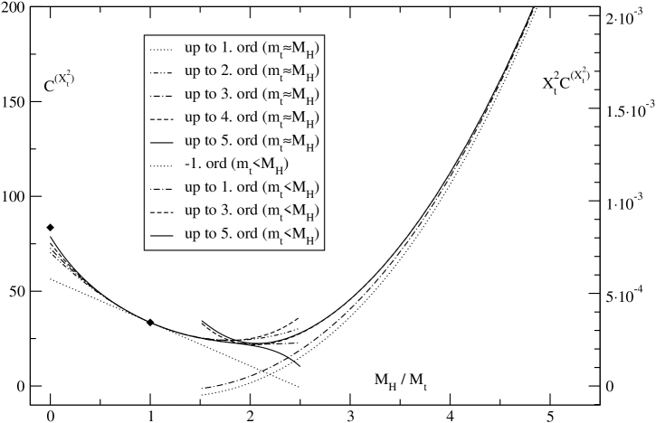
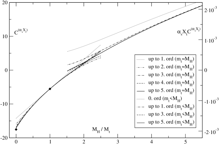
Figure 3: Contributions of order $x_{t}^{2}$ to the relation between the $\overline{\mbox{MS}}$ and on-shell top quark mass. The black squares indicate the points where the exact result is known.

Figure 4: Contributions of order $\alpha_{s}x_{t}$ to the relation between the $\overline{\mbox{MS}}$ and on-shell top quark mass. The black squares indicate the points where the exact result is known.

The results are shown in Fig. 4 and 4. A smooth transition between the two regions of large $M_{H}$ and $M_{H}\approx M_{t}$ is observed. Furthermore, the expansion around $M_{H}\approx M_{t}$, when extrapolated down to $M_{H}=0$, leads to a remarkably good agreement with the value obtained from an analytical calculation at $M_{H}=0$, a further and independent test of the approximation procedure.

The result for the ratio between $\overline{\mbox{MS}}$ mass and on-shell mass — as well as the analytical expressions for the coefficients given in sections 3 and 5 — is available from the authors upon request.

5 $\Delta\rho$ expressed through the on-shell top quark mass

Combining the results of sections 3 and 4 we compute $\Delta\rho$ in terms of the on-shell top quark mass $M_{t}$, the on-shell Higgs mass $M_{H}$ and the low energy Fermi constant $G_{F}$. Our calculation reproduces the one- and two-loop results for the $\rho$ parameter at orders $G_{F}$, $G_{F}^{2}$ and $G_{F}\alpha_{s}$ [1, 2, 3].

The result for the on-shell definition of the top quark mass is parameterized in the same way as the $\overline{\mbox{MS}}$ result in section 3. In order to distinguish the two schemes we use again the expansion parameter $X_{t}$, depending on the on-shell top quark mass $M_{t}$.

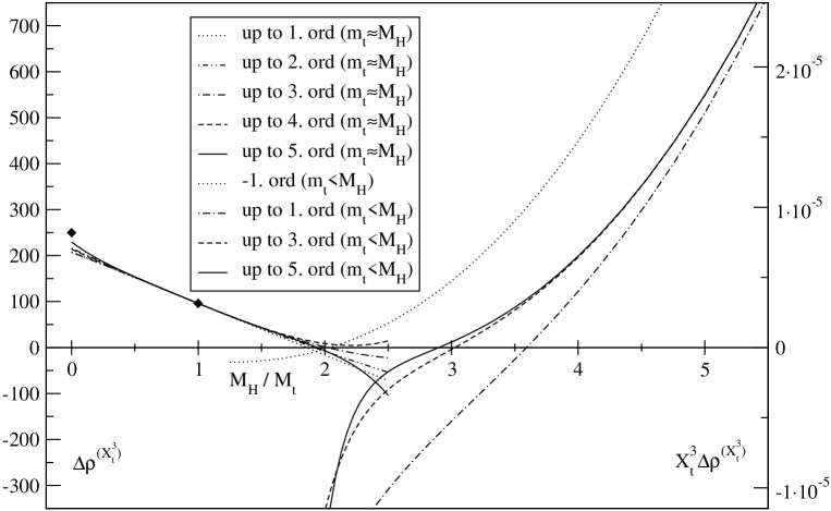
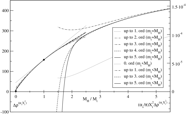
Figure 5: Contributions of order $X_{t}^{3}$ to $\Delta\rho$ in the on-shell definition of the top quark mass. The black squares indicate the points where the exact result is known.

Figure 6: Contributions of order $\alpha_{s}X_{t}^{2}$ to $\Delta\rho$ in the on-shell definition of the top quark mass. The black squares indicate the points where the exact result is known.

For completeness we also include the results for $M_{H}=0$, computed in [5]:

$$\Delta\rho^{(X_{t}^{3})} = 249.74\ ,$$ (16)

$$\Delta\rho^{(\alpha_{s}X_{t}^{2})} = 2.94\ .$$ (17)

For the expansion around $M_{H}=M_{t}$ we obtain:

$$\Delta\rho^{(X_{t}^{3})} = 95.92-111.98\delta+8.099\delta^{2}+9.36\delta^{3}+7.27\delta^{4}+-15.60\,\delta^{5}+\mathcal{O}(\delta^{6}),$$ (18)

$$\Delta\rho^{(\alpha_{s}X_{t}^{2})} = 157.295+112.00\delta-24.73\delta^{2}+7.39\delta^{3}-3.52\delta^{4}+2.06\,\delta^{5}+\mathcal{O}(\delta^{6}),$$ (19)

using $\delta$ defined by $M_{H}=M_{t}(1+\delta)$.

In the limit $M_{H}\gg M_{t}$ we obtain

$$\Delta\rho^{(X_{t}^{3})} = \frac{1}{Y}(-3.17-83.25\,\log Y)$$

$$- 189.93-231.48\,\log Y-142.06\,\log^{2}Y+2.75\,\log^{3}Y$$

$$+ Y\,\left(-332.34+77.71\,\log Y-68.67\,\log^{2}Y+51.79\,\log^{3}Y\right)$$

$$+ Y^{2}\,\left(227.55-510.55\,\log Y+87.77\,\log^{2}Y+6.41\,\log^{3}Y\right)$$

$$+ Y^{3}\,\left(-58.40-329.18\,\log Y+20.42\,\log^{2}Y+14.54\,\log^{3}Y\right)$$

$$+ Y^{4}\,\left(-36.14-381.88\,\log Y+18.63\,\log^{2}Y+15.04\,\log^{3}Y\right)$$

$$+ Y^{5}\,\left(-39.08-416.36\,\log Y+13.76\,\log^{2}Y+17.19\,\log^{3}Y\right)$$

$$+ \mathcal{O}(Y^{6}),$$

$$\Delta\rho^{(\alpha_{s}X_{t}^{2})} = 79.73-47.77\,\log Y+42.07\,\log^{2}Y+9.00\,\log^{3}Y$$

$$+ Y\,\left(225.16-179.74\,\log Y+70.22\,\log^{2}Y-19.22\,\log^{3}Y\right)$$

$$+ Y^{2}\,\left(-76.07+25.33\,\log Y-9.17\,\log^{2}Y-5.57\,\log^{3}Y\right)$$

$$+ Y^{3}\,\left(-10.10-24.69\,\log Y-0.30\,\log^{2}Y-5.46\,\log^{3}Y\right)$$

$$+ Y^{4}\,\left(-4.52-32.85\,\log Y+0.72\,\log^{2}Y-5.25\,\log^{3}Y\right)$$

$$+ Y^{5}\,\left(-2.55-36.61\,\log Y+1.06\,\log^{2}Y-5.14\,\log^{3}Y\right)$$

$$+ \mathcal{O}(Y^{6})\,,$$

with

$$Y\equiv\frac{4M_{t}^{2}}{M_{H}^{2}}\,.$$ (22)

The results in the on-shell definition of the top quark mass are shown in Fig. 6 and 6. Again, the solid line corresponds to the numerical values including all terms of our expansion. The left and right scales give the size of the coefficient and the full effect on $\Delta\rho$ respectively.

The $\alpha_{s}X_{t}^{2}$ contributions are sizeable and monotonously increasing over the full range of the Higgs mass suggesting a smoothly increasing behavior qualitatively similar to the well-known $X_{t}^{2}$ correction (displayed in Fig. 7). For $M_{H}=0$ the result seems to be accidentally small, but increases rapidly for larger Higgs mass values. The $X_{t}^{3}$ term exhibits a minimum in the range between $M_{H}=2M_{t}$ and $M_{H}=3M_{t}$ and appears to be very small or even negative in this region.

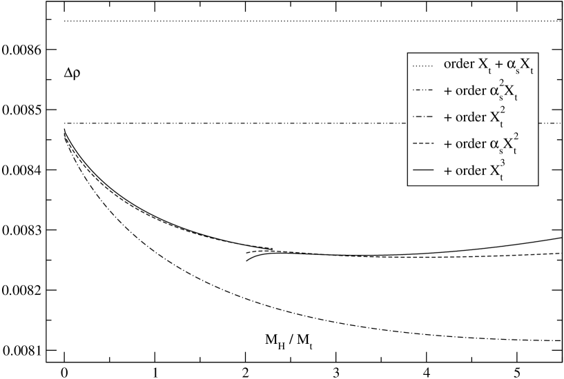
Figure 7: Effect of several contributions to $\Delta\rho$ in the on-shell definition of the top quark mass.

To compare the size of the three-loop contributions to the known one- and two-loop terms we display their individual effects on $\Delta\rho$ in Fig. 7, including the corrections of order $\alpha_{s}^{2}X_{t}$ computed in [4]. We start with the sum of the contributions of order $X_{t}$ and $\alpha_{s}X_{t}$ which are independent of the Higgs mass and proceed by adding the particular orders to $\Delta\rho$. To identify the individual contributions for $M_{H}=0$ we continued the value horizontally to the negative $M_{H}/M_{t}$ region.

Let us first consider the $\alpha_{s}X_{t}^{2}$ and $X_{t}^{3}$ terms for the case $M_{H}=0$, discussed already in [5]. Inclusion of the $\alpha_{s}X_{t}^{2}$ term leads to a change in $\Delta\rho$ of $1.0\cdot 10^{-6}$, which is not visible in Fig. 7. The $X_{t}^{3}$ term increases $\Delta\rho$ by roughly $8.2\cdot 10^{-6}$, again an extremely small effect. The picture alters drastically for larger values of $M_{H}$. The order $\alpha_{s}X_{t}^{2}$ correction is sizeable in the region of $M_{H}\approx M_{t}$ and above. It amounts to approximately $1/3$ of the two-loop contribution $\Delta\rho^{(X_{t}^{2})}$, but appears with the opposite sign. In contrast, the pure electroweak three-loop contribution $\Delta\rho^{(X_{t}^{3})}$ yields an enhancement of about 1% compared to the order $X_{t}^{2}$ terms and is therefore negligible for $M_{H}$ values of present interest.

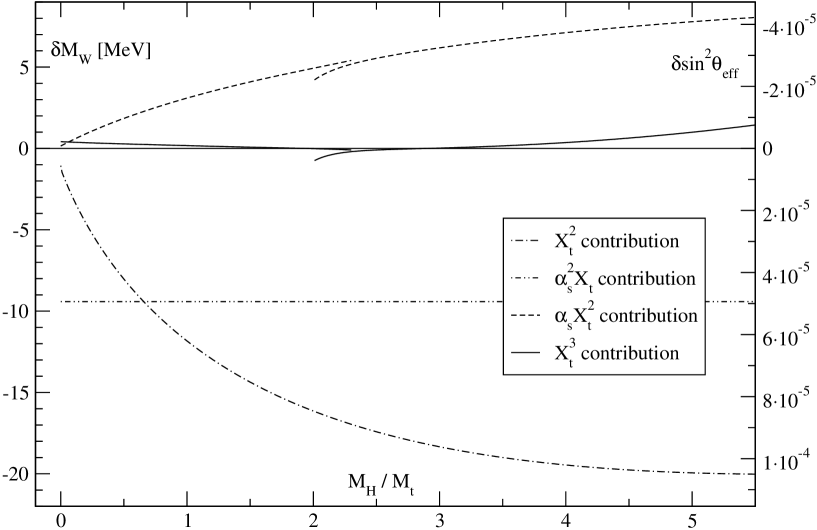
Figure 8: Shifts in $M_{W}$ and in $\sin^{2}\theta_{W}$ from the various corrections to $\Delta\rho$.

These corrections to $\Delta\rho$ can be used to examine the resulting shifts of observables like the $W$ mass and the effective weak mixing angle, predicted for fixed values of $M_{Z}$, $\alpha$, and $G_{F}$ through the equations

$$M_{W}^{2}=\frac{\rho M_{Z}^{2}}{2}\left(1+\sqrt{1-\frac{4\pi\alpha}{\sqrt{2}\rho G_{F}M_{Z}^{2}}\left(\frac{1}{1-\Delta\alpha}+\dots\right)}\right)$$ (23)

and

$$\sin^{2}\theta_{\mbox{\small eff}}=1-\frac{M_{W}^{2}}{\rho M_{Z}^{2}}=\frac{1}{2}\left(1-\sqrt{1-\frac{4\pi\alpha}{\sqrt{2}\rho G_{F}M_{Z}^{2}}\left(\frac{1}{1-\Delta\alpha}+\dots\right)}\right),$$ (24)

where $\Delta\alpha$ is the shift of $\alpha$ due to photon vacuum polarization effects and the dots are nonleading remainder terms. In Fig. 8 the resulting shifts are shown for the different orders of $\Delta\rho$ in dependence of the Higgs mass (We do not display the shift of order $\alpha_{s}X_{t}$ which amounts to $-52.8$ MeV). This shift should be compared to $\delta M_{W}=6\mbox{ MeV}$ and $\delta\sin^{2}\theta_{\rm eff}=1.3\cdot 10^{-5}$ which is the precision anticipated for TESLA operating at the $Z$-resonance [20].

Alternatively we also present the shift in $M_{t}$ which would lead to a comparable shift in $\Delta\rho$:

$$\frac{\delta M_{t}}{M_{t}}\approx\frac{1}{2}\,\frac{\delta\Delta\rho}{3X_{t}}\,.$$ (25)

For $\delta\Delta\rho=5\cdot 10^{-5}$ this leads to a shift of $m_{t}$ by about 500 MeV, which has to be compared to $\delta m_{t}\approx\mathcal{O}(100\mbox{MeV})$ anticipated for measurements at a future linear collider.

For fixed $M_{t}$, $M_{W}$, and $M_{Z}$ our result for $\Delta\rho$ has to be compensated by a shift in the prediction for $M_{H}$:

$$\frac{\delta M_{H}}{M_{H}}\approx\frac{12\sqrt{2}}{11G_{F}}\,\frac{\cos^{2}\theta_{W}}{\sin^{2}\theta_{W}}\,\delta\Delta\rho\approx 670\;\delta\Delta\rho$$ (26)

For $M_{H}$ between 120 GeV and 200 GeV the term $\alpha_{s}X_{t}^{2}$ leads to an upward shift between 4.5 and 7.5 GeV, the $X_{t}^{3}$ term to further positive shift of less than 0.5 GeV.

The $X_{t}^{2}\alpha_{s}$ term is, furthermore, comparable or larger than the non logarithmically enhanced light fermion electroweak two-loop corrections [21] and significantly larger than the purely bosonic two-loop contribution. The $X_{t}^{3}$ is comparable in size to the bosonic two-loop effects evaluated in [22].

Summary: Combining the results from the extreme regions $M_{H}=0$, $M_{H}\approx M_{t}$, and $M_{H}\gg M_{t}$ a prediction for the $X_{t}^{3}$ and $\alpha_{s}X_{t}^{2}$ contributions to the $\rho$ parameter has been obtained, which covers in a reliable way the full region of $M_{H}$. The magnitude of these terms is comparable to the non-enhanced two-loop corrections.

References

[1]
M. Veltman, Nucl. Phys. B 123 (1977) 89.
[2]
J.J. van der Bij and F. Hoogeveen, Nucl. Phys. B 283 (1987) 477;
R. Barbieri, M. Beccaria, P. Ciafaloni, G. Curci, and
A. Vicere,
Phys. Lett. B 288 (1992) 95.
[3]
J. Fleischer, O. V. Tarasov, and F. Jegerlehner, Phys. Lett. B 319 (1993) 249.
[4]
L. Avdeev, J. Fleischer, S.M. Mikhailov, and O.V. Tarasov,
Phys. Lett. B 336 (1994) 560;
E: Phys. Lett. B 349 (1995) 597;
K.G. Chetyrkin, J.H. Kühn, and M. Steinhauser, Phys. Lett. B 351 (1995) 331.
[5]
J.J. van der Bij, K.G. Chetyrkin, M. Faisst, G. Jikia, and
T. Seidensticker,
Phys. Lett. B 498 (2001) 156.
[6]
P. Nogueira, J. Comp. Phys. 105 (1993) 279.
[7]
V.A. Smirnov, Applied Asymptotic Expansions in Momenta and
Masses,
Springer-Verlag, Berlin (2002).
[8]
T. Seidensticker, hep-ph/9905298;
R. Harlander, T. Seidensticker, and M. Steinhauser, Phys. Lett. B 426 (1998) 125.
[9]
M. Steinhauser, Comp. Phys. Commun. 134 (2001) 335.
[10]
J.A.M. Vermaseren, Symbolic Manipulation with FORM, CAN (1991);
see also J.A.M. Vermaseren, math-ph/0010025.
[11]
M. Veltman, Act. Phys. Pol. B 8 (1977) 475.
[12]
R. Tarrach,
Nucl. Phys.B 183 (1981) 384.
[13]
M. Bohm, H. Spiesberger, and W. Hollik,
Fortsch. Phys.34 (1986) 687;
J. Fleischer and F. Jegerlehner,
Phys. Rev.D 23 (1981) 2001.
[14]
N. Gray, D. J. Broadhurst, W. Grafe, and K. Schilcher,
Z. Phys.C 48 (1990) 673;
J. Fleischer, F. Jegerlehner, O. V. Tarasov, and O. L. Veretin,
Nucl. Phys.B 539 (1999) 671;
Err.-ibid. B 571 (2000) 511.
[16]
J. Fleischer and M. Y. Kalmykov,
Comput. Phys. Commun.128 (2000) 531.
[17]R
Mertig and R. Scharf,
Comput. Phys. Commun.111 (1998) 265.
[18]
O. V. Tarasov,
Nucl. Phys.B 502 (1997) 455.
[19]
M. Beneke and V. A. Smirnov,
Nucl. Phys.B 522 (1998) 321.
[20]
J. A. Aguilar-Saavedra et al. [ECFA/DESY LC Physics Working Group
Collaboration],
hep-ph/0106315.
[21]
A. Freitas, S. Heinemeyer, W. Hollik, W. Walter, and G. Weiglein,
Nucl. Phys.B 632 (2002 ) 189.
[22]
M. Awramik and M. Czakon,
Phys. Rev. Lett.89 (2002) 241801;
A. Onishchenko and O. Veretin,
Phys. Lett.B 551 (2003) 111;
M. Awramik, M. Czakon, A. Onishchenko, and O. Veretin, hep-ph/0209084.