TPJU-1/2003
  
Pion Generalized Distribution Amplitudes in the Nonlocal Chiral Quark Model

Abstract

We use a simple, instanton motivated, nonlocal chiral quark model to calculate pion Generalized Distribution Amplitudes (GDAs). The nonlocality appears due to the momentum dependence of the constituent quark mass, which we take in a form of a generalized dipole formula. With this choice all calculations can be performed directly in the Minkowski space and the sensitivity to the shape of the cutoff function can be studied. We demonstrate that the model fulfills soft pion theorems both for chirally even and chirally odd GDAs. The latter one cannot be derived by the methods of current algebra. Whenever possible we compare our results with the existing data. This can be done for the pion electromagnetic form factor and quark distributions as measured in the proton-pion scattering.

1 Introduction

In this work we calculate two pion distribution amplitudes ($2\pi$DAs) and pion skewed parton distributions ($\pi$SPDs) in the instanton motivated, effective chiral quark model. $2\pi$DAs and $\pi$SPDs are defined as Fourier transforms of matrix elements of certain light-cone operators, taken between the pion states. $2\pi$DAs appear in the amplitude for the process $\gamma^{\ast}\gamma\,\rightarrow\,\pi\pi$, if the virtuality of the photon is much larger then the squared invariant mass of the two pion system [1]. $2\pi$DAs describe the transition from partons to two pions in a final state. They are also related to the pion electromagnetic form factor in the time like region and pion electromagnetic radius.

The process $\gamma^{\ast}\gamma\,\rightarrow\,\pi\pi$ can be related by crossing symmetry to virtual Compton scattering $\gamma^{\ast}\pi\,\rightarrow\,\gamma\pi$. This process factorizes into a hard photon-parton scattering and $\pi$SPDs [2]–[4]. In the forward limit the latter reduce to the quark densities which are measurable in the $\pi-$p Drell-Yan process or prompt photon production [5, 6]. Finally certain integral of $\pi$SPDs gives pion electromagnetic form factor in the space like region.

Pions are the simplest hadronic states being $q\bar{q}$ pairs and Goldstone bosons of spontaneously broken chiral symmetry at the same time. Therefore their properties may be calculated with little dynamical input, relying on their chiral structure and chiral symmetry breaking. In this work we use the instanton motivated effective chiral quark model [7] with nonlocal interactions. This model has been successfully applied to the calculation of the leading twist pion distribution amplitude [7]–[10], $2\pi$DAs [11]–[13] and pion SPDs [12, 13]. The main ingredient of the model is the momentum dependence of the constituent quark mass which regularizes certain, otherwise divergent, integrals. To make the calculation feasible this momentum dependence has been taken in the form [9] :

$$M_{k}=M\left(\frac{-\Lambda^{2}}{k^{2}-\Lambda^{2}+i\epsilon}\right)^{2n}=MF^{2}(k).$$ (1)

$M$ is the constituent quark mass at zero momentum. Its value, obtained from the gap equation, is approximately $350$ MeV. Quantities $n$ and $\Lambda=\Lambda(n;M)$ are model parameters. As explained below we expect the model to be roughly independent of $n$, if the value of $\Lambda$ is properly adjusted. The formula (1) maybe thought to be instanton motivated in a sense, that when continued to Euclidean momenta ($k^{2}\,\rightarrow\,-k_{E}^{2}$), it reproduces reasonably well [9] the momentum dependence calculated explicitly [14, 15] in the instanton model of the QCD vacuum:

$$F_{\mbox{{\small inst}}}(k_{E})=2z[I_{0}(z)K_{1}(z)-I_{1}(z)K_{0}(z)]-2I_{1}(z)K_{1}(z),$$ (2)

where $z=\rho k_{E}/2$, with $\rho=(600~{}\mbox{MeV})^{-1}$ being an average instanton size.

The calculations presented here may be viewed as an extension of the previous results of Refs.[11]–[13] and were partially reported in [16, 17]. Our motivations are both theoretical and phenomenological. First, the asymptotics of Eq.(2) suggests $n=3/2$ in Eq.(1), however, taking the non-integer $n$ results in additional difficulties. In the previous works [7, 8, 11]–[13] the value $n=1$ was assumed. Therefore it should be checked that the results do not depend strongly on $n$. This is indeed true for the pion distribution amplitude, as has been shown in [9]. Secondly in [7, 8, 11]–[13] the momentum dependence of the constituent mass in the quark propagators was neglected. With the method developed in [9] we can calculate generalized parton distributions for arbitrary $n$, keeping track of momentum dependence of the constituent quark mass both in numerators and denominators even for the convergent quantities. This is in fact necessary if one insists on the soft pion theorems which would be otherwise not fulfilled. Apart from a well known soft pion theorem for a chirally even $2\pi$DA [12], we derive (in the framework of the present model) a soft pion theorem for a chirally odd $2\pi$DA.

On the phenomenological side, apart from the calculation of the pion generalized distribution amplitudes (GDAs for short), i.e. $2\pi$DAs and $\pi$SPDs themselves, we calculate pion electromagnetic radius, electromagnetic form factor and quark distributions, and compare them with the existing data. This comparison although not bad, is not entirely satisfactory. We shall discuss our results in Sect.7. We start with the short description of the model in Sect.2 Then, in Sect.3, we proceed with definitions of $2\pi$DAs and $\pi$SPDs and their general properties. In Sect.4 we sketch the calculations and present numerical results. In Sect.5 we demonstrate soft pion theorems. Finally, in Sect.6, we discuss pion quark densities calculated in the model and compare them with data and other theoretical calculations. Technical details can be found in the Appendix.

2 Effective chiral quark model

For two quark flavors ($u$ and $d$) the effective model we use to calculate pion GDAs is given by the action (in momentum space):

$$S_{eff}=\int\frac{d^{4}k}{(2\pi)^{4}}\,\bar{\psi}(k)\hbox to0.0pt{/\hss}k\,\psi(k)-\int\frac{d^{4}p}{(2\pi)^{4}}\frac{d^{4}k}{(2\pi)^{4}}\,\bar{\psi}(p)\sqrt{M_{p}}U^{\gamma_{5}}(p-k)\sqrt{M_{k}}\psi(k),$$ (3)

where

$$\psi(x)=\int\frac{d^{4}k}{(2\pi)^{4}}e^{-i\,kx}\psi(k).$$

The matrix

$$U^{\gamma_{5}}(x)=\exp\left[\frac{i}{F_{\pi}}\gamma^{5}\tau^{a}\pi^{a}(x)\right]=1+\frac{i}{F_{\pi}}\gamma^{5}\tau^{a}\pi^{a}(x)-\frac{1}{2F_{\pi}^{2}}\pi^{a}(x)\pi^{a}(x)+\ldots$$ (4)

(in coordinate space) gives the interaction between quarks and pions. There is no kinetic term for the pions and the pion field is treated as an external source. $F_{\pi}=93$ MeV is the pion decay constant, $\tau^{a}$ are Pauli matrices and the pion $\hat{T}_{3}$ eigen states are: $\pi^{0}=\pi^{3}$, $\pi^{+}=-\left(\pi^{1}+i\pi^{2}\right)/\sqrt{2}$, $\pi^{-}=\left(\pi^{1}-i\pi^{2}\right)/\sqrt{2}$. The momentum dependence of the quark constituent mass is given by Eq.(1). The $\Lambda$ parameter is fixed once for all by adjusting the value of $F_{\pi}(\Lambda)$ calculated in the effective model (3) to its physical value $F_{\pi}=93$ MeV. This has been done in [9]. For example for $M=350$ MeV and $n=1$ we have obtained $\Lambda=1157$ MeV.

Neither $M$ nor $\Lambda$ should be identified with the normalization scale $Q_{0}$ of the quantities calculated in the model. The precise definition of $Q_{0}$ is only possible within QCD and in all effective models one can use only qualitative order of magnitude arguments to estimate $Q_{0}$. Arguments can be given that the characteristic scale of the instanton model is of the order of the inverse instanton size $1/\rho=600$ MeV, or so. We shall come back to this question in Sect.6.

3 Definitions and general properties of GDAs

We define two light-like vectors: $n^{\mu}=(1,0,0,-1)$ and $\tilde{n}^{\mu}=(1,0,0,1)$. These vectors define plus and minus components of any four-vector: $k^{+}\equiv k^{0}+k^{3}=n\cdot k$ and $k^{-}\equiv k^{0}-k^{3}=\tilde{n}\cdot k$.

3.1 Two pion distribution amplitudes

We take the definitions of pion generalized distribution amplitudes from [12, 13].

$$\int\frac{d\lambda}{2\pi}\exp\left(-iu\lambda n\cdot P\right)\left\langle\pi^{a}(p_{1})\pi^{b}(p_{2})\left|\bar{\psi}^{f^{\prime}}(\lambda n)\Gamma\psi^{f}(0)\right|0\right\rangle$$

$$=\delta^{ab}\,\delta^{ff^{\prime}}\,\Phi_{2\pi}^{I=0}(u,v,s)+i\varepsilon^{abc}\,(\tau^{c})^{ff^{\prime}}\,\Phi_{2\pi}^{I=1}(u,v,s),$$ (5)

where $P=p_{1}+p_{2}$ is the total momentum of the two pion system. For the leading twist (chirally even) $2\pi$DAs we have:

$$\Gamma=\hbox to0.0pt{/\hss}n,$$ (6)

whereas for the chirally odd $2\pi$DAs

$$\Gamma=in^{\alpha}P^{\beta}\sigma_{\alpha\beta}.$$ (7)

Note that with the definition (7), chirally odd $2\pi$DAs have the dimension of mass. $2\pi$DAs depend on the following kinematical variables: squared invariant mass of the two pions, $s=P^{2}$; the longitudinal momentum fraction carried by quark with respect to the total longitudinal momentum, $u=k^{+}/P^{+}$ and the longitudinal momentum fraction carried by one of the pions with respect to the total longitudinal momentum, $v=p_{1}^{+}/P^{+}$.

$2\pi$DAs have the following symmetries [12]:

$$\Phi_{2\pi}^{I=0}(u,v,s)=-\Phi_{2\pi}^{I=0}(1-u,v,s)=\Phi_{2\pi}^{I=0}(u,1-v,s),$$ (8)

$$\Phi_{2\pi}^{I=1}(u,v,s)=\Phi_{2\pi}^{I=1}(1-u,v,s)=-\Phi_{2\pi}^{I=1}(u,1-v,s).$$ (9)

The isovector chirally even $2\pi$DA is normalized to the pion electromagnetic form factor in the time-like region:

$$\int\limits_{0}^{1}du\,\Phi_{2\pi}^{I=1}(u,v,s)=(1-2v)F_{\pi}^{\mbox{{\small em}}}(s).$$ (10)

From its $s$ dependence the pion electromagnetic radius can be evaluated

$$\langle(r_{\pi}^{em})^{2}\rangle=6\left.\frac{dF_{\pi}^{\mbox{{\small em}}}(s)}{ds}\right|_{s=0}.$$ (11)

The normalization condition for the isoscalar $2\pi$DA gives the fraction of a pion momentum carried by the quarks, $M_{2}^{(\pi)}$:

$$\int\limits_{0}^{1}du\,(2u-1)\Phi_{2\pi}^{I=0}(u,v,s=0)=-2v(1-v)M_{2}^{(\pi)}.$$ (12)

It is convenient do expand the $2\pi$DAs in the basis of the eigen functions of the ERBL equation [18, 19] (Gegenbauer polynomials $C_{n}^{3/2}(2u-1)$) and partial waves of scattered pions (Legendre polynomials $P_{l}(1-2v)$):

$$\Phi_{2\pi}^{I}(u,v,s)=6u(1-u)\sum_{n=0}^{\infty}\sum_{l=0}^{n+1}B_{nl}^{I}(s)C_{n}^{3/2}(2u-1)P_{l}(1-2v).$$ (13)

Because of the symmetry properties (8, 9), the sum in Eq.(13) goes over odd (even) $n$ and even (odd) $l$ for isoscalar (isovector) $2\pi$DA.

The expansion coefficients $B_{nl}^{I}$ are renormalized multiplicatively:

$$B_{nl}^{I}(s;Q)=B_{nl}^{I}(s;Q_{0})\left(\frac{\alpha_{s}(Q)}{\alpha_{s}(Q_{0})}\right)^{\gamma_{n}},$$ (14)

with $\gamma_{n}$ being anomalous dimensions [20]. From (13) and (14) it is easy to read the asymptotic form of $2\pi$DAs:

$$\Phi_{2\pi}^{\mbox{\small as.}\,I=0}(u,v,s)=0$$ (15)

and

$$\Phi_{2\pi}^{\mbox{\small as.}\,I=1}(u,v,s)=6u(1-u)(1-2v)B_{01}^{I=1}(s).$$ (16)

This asymtotic form is plotted in Fig.1. For chirally even $2\pi$DA, from (10), we have $B_{01}^{I=1}(s)=F_{\pi}^{\mbox{\small em}}(s)$.

\psfrag{s}{$s=0$~{}GeV${}^{2}$}\psfrag{u}{~{}}\psfrag{v}{~{}}\psfrag{quark}{\footnotesize quark $u$}\psfrag{pion}{\footnotesize pion $v$}\includegraphics[scale={0.6}]{gda_fig_01.eps}

Figure 1: Asymptotic form the isovector 2$\pi$DA as given by Eq.(16).

In Ref.[12] the following soft pion theorem for the chirally even $2\pi$DAs has been demonstrated. In the chiral limit ($m_{\pi}=0$), in the case of one of the pions momenta going to zero ($v(1-v)\rightarrow 0$) we get

$$\Phi_{2\pi}^{I=0}(u,v=0,s=0)=\Phi_{2\pi}^{I=0}(u,v=1,s=0)=0$$ (17)

and

$$\Phi_{2\pi}^{I=1}(u,v=0,s=0)=-\Phi_{2\pi}^{I=1}(u,v=1,s=0)=\phi_{\pi}^{AV}(u),$$ (18)

where $\phi_{\pi}^{AV}(u)$ is the axial-vector (leading twist) pion distribution amplitude:

$$\langle 0|\bar{d}(z)\gamma_{\mu}\gamma_{5}u(-z)|\pi^{+}(p)\rangle=i\sqrt{2}F_{\pi}p_{\mu}\int\limits_{0}^{1}du\,e^{i(2u-1)z\cdot p}\phi_{\pi}^{AV}(u).$$ (19)

We shall come back to this point in Sect.5.

3.2 Pion skewed distributions

For $\pi$SPDs we have (for a review see Ref.[4]):

$$\frac{1}{2}\int\frac{d\lambda}{2\pi}\exp\left(i\lambda Xn\cdot\bar{p}\right)\left\langle\pi^{b}(p^{\prime})\left|\bar{\psi}^{f^{\prime}}\left(-\frac{\lambda n}{2}\right)\hbox to0.0pt{/\hss}n\psi^{f}\left(\frac{\lambda n}{2}\right)\right|\pi^{a}(p)\right\rangle$$

$$=\delta^{ab}\,\delta^{ff^{\prime}}\,H^{I=0}(X,\xi,t)+i\varepsilon^{abc}\,\left(\tau^{c}\right)^{ff^{\prime}}\,H^{I=1}(X,\xi,t),$$ (20)

where $\bar{p}=(p+p^{\prime})/2$ is the average pion momentum. SPDs depend on the following kinematical variables: the asymmetry parameter $\xi=-\Delta^{+}/(2\bar{p}^{+})$, where $\Delta=p^{\prime}-p$ is the four-momentum transfer; $t=\Delta^{2}$ and the variable $X$ defining the longitudinal momenta of the struck and scattered quarks in DVCS, $(X+\xi)\bar{p}^{+}$ and $(X-\xi)\bar{p}^{+}$ respectively.

The pion SPDs obey the following symmetry properties [13]:

$$H^{I=0}(X,\xi,t)=H^{I=0}(X,-\xi,t)=-H^{I=0}(-X,\xi,t),$$ (21)

$$H^{I=1}(X,\xi,t)=H^{I=1}(X,-\xi,t)=H^{I=1}(-X,\xi,t).$$ (22)

In the forward limit the SPDs reduce to the usual quark and antiquark distributions:

$$H^{I=0}(X,\xi=0,t=0)=\frac{1}{2}\left[\Theta(X)q_{s}(X)-\Theta(-X)q_{s}(-X)\right],$$ (23)

$$H^{I=1}(X,\xi=0,t=0)=\frac{1}{2}\left[\Theta(X)q_{v}(X)+\Theta(-X)q_{v}(-X)\right],$$ (24)

where $q_{s}(X)$, $q_{v}(X)$ are singlet (quark plus antiquark) and valence (quark minus antiquark) distributions. For example for $\pi^{+}$ we have:

$$2H^{I=0}(X,\xi=0,t=0)=\left\{\begin{array}[]{rcc}u^{\pi^{+}}(X)+\bar{u}^{\pi^{+}}(X)&\mbox{for}&X>0,\\ -d^{\pi^{+}}(-X)-\bar{d}^{\pi^{+}}(-X)&\mbox{for}&X<0\end{array}\right.$$ (25)

and

$$2H^{I=1}(X,\xi=0,t=0)=\left\{\begin{array}[]{rcc}u^{\pi^{+}}(X)-\bar{u}^{\pi^{+}}(X)&\mbox{for}&X>0,\\ -d^{\pi^{+}}(-X)+\bar{d}^{\pi^{+}}(-X)&\mbox{for}&X<0.\end{array}\right.$$ (26)

In the present model we get $\bar{u}^{\pi^{+}}(X)=d^{\pi^{+}}(X)\equiv 0$.

The normalization conditions for SPDs are analogous to the $2\pi$DAs case (10, 11, 12). In particular

$$\int\limits_{-1}^{+1}dX\,H^{I=1}(X,\xi,t)=F_{\pi}^{\mbox{{\small em}}}(t),$$ (27)

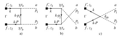
Figure 2: Diagrams contributing to the matrix element $\left\langle\pi^{a}(p_{1})\pi^{b}(p_{2})\left|\bar{\psi}^{f^{\prime}}(z_{1})\Gamma\psi^{f}(z_{2})\right|0\right\rangle$, Eq.(5). Diagrams a) and b) contribute both to isoscalar and isovector $2\pi$DAs; diagram c) contributes only to the isoscalar $2\pi$DA.

$$\langle(r_{\pi}^{em})^{2}\rangle=6\left.\frac{dF_{\pi}^{\mbox{{\small em}}}(t)}{dt}\right|_{t=0}$$ (28)

and

$$\int\limits_{-1}^{+1}dX\,XH^{I=0}(X,\xi,t=0)=\frac{1}{2}(1-\xi^{2})M_{2}^{(\pi)}.$$ (29)

In analogy to the soft pion theorem for $2\pi$DAs, in the case of $\pi$SPD we have [12]:

$$H^{I=1}(X,\xi=1,t=0)=\phi_{\pi}^{AV}\left(\frac{X+1}{2}\right),\qquad H^{I=0}(X,\xi=1,t=0)=0.$$ (30)

4 Pion generalized distribution amplitudes in the effective model

4.1 Analytical results

For the matrix elements entering the definitions of $2\pi$DAs and SPDs, Eqs.(5,3.2), in the effective model described in Sect.2, we obtain:

$$\left\langle\pi^{a}(p_{1})\pi^{b}(p_{2})\left|\bar{\psi}^{f\prime}(z_{1})\Gamma\psi^{f}(z_{2})\right|0\right\rangle=i\frac{N_{C}}{F_{\pi}^{2}}\int\frac{d^{4}k}{(2\pi)^{4}}e^{ikz_{1}-i(k-P)z_{2}}$$

$$\left\{\delta^{ab}\delta^{ff^{\prime}}\left[\mathcal{T}_{1}(k-P,k)+\mathcal{T}_{2}\left(k-P,k-p_{2},k\right)+\mathcal{T}_{2}\left(k-P,k-p_{1},k\right)\right]\right.$$

$$\left.+i\varepsilon^{abc}\,(\tau^{c})^{ff^{\prime}}\left[\mathcal{T}_{2}\left(k-P,k-p_{2},k\right)-\mathcal{T}_{2}\left(k-P,k-p_{1},k\right)\right]\right\},$$ (31)

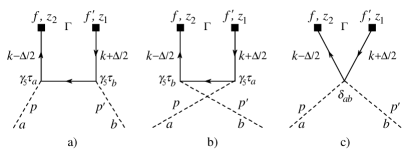
Figure 3: Diagrams contributing to the matrix element $\left\langle\pi^{b}(p^{\prime})\left|\bar{\psi}^{f^{\prime}}(z_{1})\Gamma\psi^{f}(z_{2})\right|\pi^{a}(p)\right\rangle$, Eq. (3.2). Diagrams a) and b) contribute both to isoscalar and isovector SPDs; diagram c) contributes only to the isoscalar SPD.

and

$$\left\langle\pi^{b}(p^{\prime})\left|\bar{\psi}^{f^{\prime}}(z_{1})\Gamma\psi^{f}(z_{2})\right|\pi^{a}(p)\right\rangle=i\frac{N_{C}}{F_{\pi}^{2}}\int\frac{d^{4}k}{(2\pi)^{4}}e^{i\left(k+\frac{\Delta}{2}\right)z_{1}-i\left(k-\frac{\Delta}{2}\right)z_{2}}$$

$$\left\{\delta^{ab}\delta^{ff^{\prime}}\left[\mathcal{T}_{1}\left(k-\frac{\Delta}{2},k+\frac{\Delta}{2}\right)\right.\right.$$ (32)

$$\qquad\qquad\left.+\mathcal{T}_{2}\left(k-\frac{\Delta}{2},k-\bar{p},k+\frac{\Delta}{2}\right)+\mathcal{T}_{2}\left(k-\frac{\Delta}{2},k+\bar{p},k+\frac{\Delta}{2}\right)\right]$$

$$\left.+i\varepsilon^{abc}\,\left(\tau^{c}\right)^{ff^{\prime}}\left[\mathcal{T}_{2}\left(k-\frac{\Delta}{2},k-\bar{p},k+\frac{\Delta}{2}\right)-\mathcal{T}_{2}\left(k-\frac{\Delta}{2},k+\bar{p},k+\frac{\Delta}{2}\right)\right]\right\},$$

where

$$\mathcal{T}_{1}(q,k)=\mbox{Tr}\left[\Gamma\frac{1}{\hbox to0.0pt{/\hss}q-M_{q}+i\epsilon}\sqrt{M_{q}M_{k}}\frac{1}{\hbox to0.0pt{/\hss}k-M_{k}+i\epsilon}\right],$$ (33)

$$\mathcal{T}_{2}(r,q,k)=\mbox{Tr}\left[\Gamma\frac{\sqrt{M_{r}}}{\hbox to0.0pt{/\hss}r-M_{r}+i\epsilon}\gamma^{5}\frac{M_{q}}{\hbox to0.0pt{/\hss}q-M_{q}+i\epsilon}\gamma^{5}\frac{\sqrt{M_{k}}}{\hbox to0.0pt{/\hss}k-M_{k}+i\epsilon}\right].$$ (34)

For the leading twist chirally even distributions $\Gamma=\hbox to0.0pt{/\hss}n$.

Equation (32) is obtained, due to the crossing symmetry, from (31) by the exchange $p_{1}\rightarrow-p$ and $p_{2}\rightarrow p^{\prime}$ (that is $P\rightarrow\Delta$). The diagrams contributing to the matrix elements (31) and (32) are shown in figures 2 and 3 respectively. The diagrams a) and b) contribute both to the isoscalar and isovector GDAs, while the diagram c) contributes only to the isoscalar GDAs.

In the case of $2\pi$DAs we will work in the reference frame defined by $\vec{P}_{\perp}=0$. In this frame we find:

$$P=\left(P^{+},\,\frac{s}{P^{+}},\,\vec{0}_{\bot}\right),$$ (35)

$$p_{1}=\left(vP^{+},\,(1-v)\frac{s}{P^{+}},\,\vec{p}_{\bot}\right),\qquad p_{2}=\left((1-v)P^{+},\,v\frac{s}{P^{+}},\,-\vec{p}_{\bot}\right),$$ (36)

$$p_{\bot}^{2}=v(1-v)s-m_{\pi}^{2}.$$ (37)

From $p_{\bot}^{2}\geq 0$ it follows

$$1-\sqrt{1-\frac{4m_{\pi}^{2}}{s}}\leq 2v\leq 1+\sqrt{1-\frac{4m_{\pi}^{2}}{s}},\qquad s\geq 4m_{\pi}^{2}.$$ (38)

In the case of pion SPDs we will work in the reference frame defined by $\vec{\bar{p}}_{\perp}=0$. In this frame we find:

$$\bar{p} =\left(\bar{p}^{+},\,\frac{-t+4m_{\pi}^{2}}{4\bar{p}^{+}},\,\vec{0}_{\bot}\right)=\left(\bar{p}^{+},\,\frac{-\tilde{t}}{4\bar{p}^{+}},\,\vec{0}_{\bot}\right),$$ (39)

$$\Delta =\left(-2\xi\bar{p}^{+},\,\xi\frac{-t+4m_{\pi}^{2}}{2\bar{p}^{+}},\,\vec{\Delta}_{\bot}\right)=\left(-2\xi\bar{p}^{+},\,\xi\frac{-\tilde{t}}{2\bar{p}^{+}},\,\vec{\Delta}_{\bot}\right),$$ (40)

$$\Delta_{\bot}^{2} =-t-\xi^{2}(-t+4m_{\pi}^{2})=(1-\xi^{2})(-\tilde{t})-4m_{\pi}^{2}.$$ (41)

From $\Delta_{\bot}^{2}\geq 0$ it follows

$$-\frac{\sqrt{-t}}{\sqrt{-t+4m_{\pi}^{2}}}\leq\xi\leq\frac{\sqrt{-t}}{\sqrt{-t+4m_{\pi}^{2}}}.$$ (42)

In what follows we take the chiral limit, $m_{\pi}=0$. In this limit, from (38) and (42), we get $0\leq v\leq 1$ and $-1\leq\xi\leq 1$.

Inserting Eqs.(31) and (32) into Eqs.(5) and (3.2) we find $k^{+}=uP^{+}$ and $k^{+}=X\bar{p}^{+}$ respectively.

The method of evaluating $dk^{-}$ integral, taking the full care of the momentum mass dependence, has been given in [9]. To evaluate $dk^{-}$ integral we have to find the poles in the complex $k^{-}$ plane. It is important to note that the poles come only from momentum dependence in the denominators of Eqs.(33,34). Indeed, for each quark line with the momentum $k$, in the case $M_{k}\rightarrow\infty$ we have at most $M_{k}$ in the numerator (if the line is coupled to pion lines at both ends) and $M_{k}$ in the denominator. This means that the position of the poles is given by the zeros of denominator, that is by the solutions of the equation

$$k^{2}-M^{2}\left(\frac{\Lambda^{2}}{k^{2}-\Lambda^{2}+i\epsilon}\right)^{4n}+i\epsilon=0.$$ (43)

This equation is equivalent to

$$G(z)=z^{4n+1}+z^{4n}-r^{2}=\prod_{i=1}^{4n+1}(z-z_{i}),$$ (44)

with $z=k^{2}/\Lambda^{2}-1+i\epsilon$ and $r^{2}=M^{2}/\Lambda^{2}$. For $r^{2}\neq 0$ (or finite $\Lambda$) equation (44) has $4n+1$ nondegenerate solutions. In general case $4n$ of them can be complex and the care must be taken about the integration contour in the complex $k^{-}$ plane. Because of the imaginary part of the $z_{i}$’s, the poles in the complex $k^{-}$ plane can drift across Re$k^{-}$ axis. In this case the contour has to be modified in such a way that the poles are not allowed to cross it. This follows from the analyticity of the integrals in the $\Lambda$ parameter and ensures the vanishing of GDAs in the kinematically forbidden regions. We get nonvanishing results for $2\pi$DAs and SPDs for $0\leq u\leq 1$ and $-1\leq X\leq 1$ respectively.

$s=0$ GeV²                                $s=1$ GeV²

\psfrag{u}{~{}}\psfrag{v}{~{}}\psfrag{quark}{\footnotesize quark $u$}\psfrag{pion}{\footnotesize pion $v$}\includegraphics[scale={0.5}]{gda_fig_04a.eps}

\psfrag{u}{~{}}\psfrag{v}{~{}}\psfrag{quark}{\footnotesize quark $u$}\psfrag{pion}{\footnotesize pion $v$}\includegraphics[scale={0.5}]{gda_fig_04b.eps}

\psfrag{u}{~{}}\psfrag{v}{~{}}\psfrag{quark}{\footnotesize quark $u$}\psfrag{pion}{\footnotesize pion $v$}\includegraphics[scale={0.5}]{gda_fig_04c.eps}

\psfrag{u}{~{}}\psfrag{v}{~{}}\psfrag{quark}{\footnotesize quark $u$}\psfrag{pion}{\footnotesize pion $v$}\includegraphics[scale={0.5}]{gda_fig_04d.eps}

Figure 4: Chirally even isoscalar (upper row) and isovector (lower row) 2$\pi$DA’s for $M=350$ MeV and $n=1$ for two different invariant masses of outgoing pions’ momenta. Note that for small $s$ and $v=0$ the isovector 2$\pi$DA resembles – as function of $u$ – the axial-vector one pion distribution amplitude in agreement with the soft pion theorem (18,63)

After evaluating $dk^{-}$ integral the $d^{2}k_{\perp}$ integral has to be treated numerically. The integral over angular dependence in the transverse plane can be in principle evaluated analytically (using residue technique), or in other words an exact algorithm for its evaluation can be given. In this way we are left with the numerical integration in only one variable, which is an easy task to do. The technical details of the calculations are presented in Appendix A.

$s=0$ GeV²                                $s=1$ GeV²

\psfrag{u}{~{}}\psfrag{v}{~{}}\psfrag{quark}{\footnotesize quark $u$}\psfrag{pion}{\footnotesize pion $v$}\includegraphics[scale={0.5}]{gda_fig_05a.eps}

\psfrag{u}{~{}}\psfrag{v}{~{}}\psfrag{quark}{\footnotesize quark $u$}\psfrag{pion}{\footnotesize pion $v$}\includegraphics[scale={0.5}]{gda_fig_05b.eps}

\psfrag{u}{~{}}\psfrag{v}{~{}}\psfrag{quark}{\footnotesize quark $u$}\psfrag{pion}{\footnotesize pion $v$}\includegraphics[scale={0.5}]{gda_fig_05c.eps}

\psfrag{u}{~{}}\psfrag{v}{~{}}\psfrag{quark}{\footnotesize quark $u$}\psfrag{pion}{\footnotesize pion $v$}\includegraphics[scale={0.5}]{gda_fig_05d.eps}

Figure 5: Chirally odd isoscalar (upper row) and isovector (lower row) 2$\pi$DA’s for $M=350$ MeV and $n=1$ for two different invariant masses of outgoing pions’ momenta. Note that for small $s$ and $v=0$ the shape in $u$ of the isoscalar 2$\pi$DA resembles the derivative (straight line) of the pseudo-tensor one pion distribution amplitude in agreement with the soft pion theorem (68).

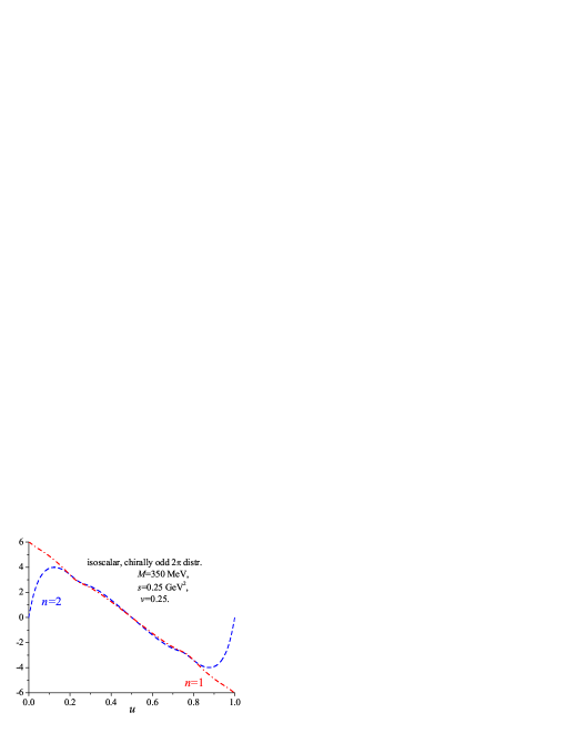
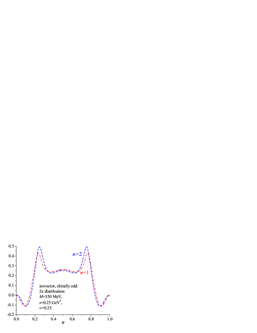
Figure 6: Isoscalar (left) and isovector (right) chirally odd 2$\pi$DA in the chiral limit for $M=350$ MeV, $n=1$ (dashed-dotted) and $2$ (dashed line), $s=0.25$ GeV², at $v=0.25$.

4.2 Numerical results

Our results for $2\pi$DAs and SPDs are presented in Figs. 4-7. Although strictly speaking the present model is valid only for small pion momenta, $s$, we show also results for $s$ as large as 1 GeV in order to trace the trends of the change of shape.

For small $s$ and one pion momentum equal zero (i.e. $v=0$) the shape of the chirally even isovector 2$\pi$DA resembles – as function of $u$ – the axial-vector one pion distribution amplitude in agreement with the soft pion theorem (18,63). Similarly, chirally odd isoscalar 2$\pi$DA resembles the derivative (straight line) of the pseudo-tensor one pion distribution amplitude, also in agreement with the soft pion theorem (68) which we shall discuss in detail in Sect.5. The functions that we obtain, obey correct symmetry properties (8, 9) and (21, 22). The asymptotic form for the isovector 2$\pi$DA is plotted in Fig.1 and we see that it has a different shape from the model prediction of Fig.4.

As in the case of the pion distribution amplitude [9] the $n$ dependence (see Eq.(1)) of our results is weak. This is depicted in Fig.6 where we plot chirally odd 2$\pi$DA’s for $M=350$ MeV and $n=1$ and 2, $s=0.25$ GeV², at $v=0.25$. One can see that there is almost no $n$ dependence except for the end point behavior of the isoscalar distribution which vanishes at $u=0,1$ for all $n>1$. This kind of behavior has been already discussed in Ref.[10] in the context of the pseudo-scalar one pion DA. The $n$ dependence of the chirally even 2$\pi$DA is similarly weak.

Skewed pion distributions for $M=350$ MeV and $n=1$ are plotted in Fig.7 for two values of $t=0$ and $-1$ GeV². Note that we only plot them for $0<\xi<1$, the remainder in region of $-1<\xi<0$ is symmetric according to Eqs.(22,21). In the present model

$$H^{I=1}(X,\,\xi=0,\,t=0)=\left\{\begin{array}[]{rcc}H^{I=0}(X,\,\xi=0,\,t=0)&\mbox{for}&X>0\\ -H^{I=0}(X,\,\xi=0,\,t=0)&\mbox{for}&X<0\end{array}\right.$$ (45)

and from (23, 24) it follows that $q_{s}(X)=q_{v}(X)$. The section of $H^{I=0}(X,\xi,t)$ as function of $X$ is plotted in Fig.8. In Fig.8.a we plot $H^{I=0}(X,\xi=0.5,t=-0.25~{}{\rm GeV}^{2})$ for $M=350$ MeV and $n=1$. The solid curve corresponds to the full result, whereas the dashed-dotted curve corresponds to diagrams a)+b) of Fig.3, and dashed line to diagram c). In the forward limit ($t=0$ and $\xi=0$, Fig.8.b) $H^{I=0}(X,\xi=0,t=0)$ corresponds to the quark densities in the pion (25). We see little $n$ dependence. For comparison we also plot quark distributions obtained in the model with sharp cutoff in the transverse momentum plane which coincides with the result obtained in Refs.[21, 22]. These quark distributions are understood to be at low normalization scale $Q_{0}$ and have to be evolved to some physical scale $Q$ at which they are experimentally accessible. This will be done in Sect.6.

Our skewed distributions do not exhibit factorization [23] and for $\xi=0$ they are quite similar in shape to the distributions obtained from local duality [24].

\psfrag{X}{\footnotesize$X$}\psfrag{xi}{\footnotesize$\xi$}\psfrag{t}{\footnotesize$t=0$~{}GeV${}^{2}$}\psfrag{t1}{\footnotesize$t=-1$~{}GeV${}^{2}$}\includegraphics[scale={0.5}]{gda_fig_07a.eps}

\psfrag{X}{\footnotesize$X$}\psfrag{xi}{\footnotesize$\xi$}\psfrag{t}{\footnotesize$t=0$~{}GeV${}^{2}$}\psfrag{t1}{\footnotesize$t=-1$~{}GeV${}^{2}$}\includegraphics[scale={0.5}]{gda_fig_07b.eps}

\psfrag{X}{\footnotesize$X$}\psfrag{xi}{\footnotesize$\xi$}\psfrag{t}{\footnotesize$t=0$~{}GeV${}^{2}$}\psfrag{t1}{\footnotesize$t=-1$~{}GeV${}^{2}$}\includegraphics[scale={0.5}]{gda_fig_07c.eps}

\psfrag{X}{\footnotesize$X$}\psfrag{xi}{\footnotesize$\xi$}\psfrag{t}{\footnotesize$t=0$~{}GeV${}^{2}$}\psfrag{t1}{\footnotesize$t=-1$~{}GeV${}^{2}$}\includegraphics[scale={0.5}]{gda_fig_07d.eps}

Figure 7: Isovector (upper row) and isoscalar (lower row) pion SPD, $H^{I=1,0}(X,\xi,t)$, in the chiral limit ($m_{\pi}=0$) for $M=350$ MeV; for $t=0$ and $-1$ GeV².

The values of $F_{\pi}^{\mbox{{\small em}}}(s)$ and $F_{\pi}^{\mbox{{\small em}}}(t)$ evaluated by means of Eqs.(10,27) do not depend (as they should) on $v$ and $\xi$ respectively. They are depicted in Fig.9, together with the experimental data of Refs. [25]-[27]. We see that the space like pion form factor overshoots the experimental points. This discrepancy may be eventually cured by negative contribution from the pion loops. In the time like region we see that very soon the $\rho$ resonance tail switches on. Of course vector mesons are not accounted for in the present model. The similar buildup of the $\rho$ tail can be seen in the $\pi-\pi$ scattering data [28]. One should note that strictly speaking our model can be used only for very low momentum transfers. For higher momenta QCD perturbative techniques should be used [29]

The values of the pion electromagnetic radius, obtained from Eqs.(11) and (28) are consistent with each other, although too small. Numerically we get $\langle(r_{\pi}^{em})^{2}\rangle=(0.54\mbox{ fm})^{2}$, which is comparable with the value

$$\langle(r_{\pi}^{em})^{2}\rangle=\frac{N_{C}}{4\pi^{2}F_{\pi}^{2}}=(0.58\mbox{ fm})^{2},$$

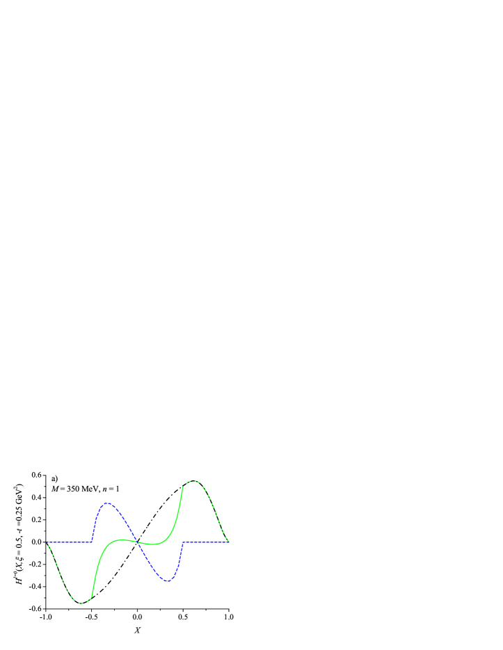
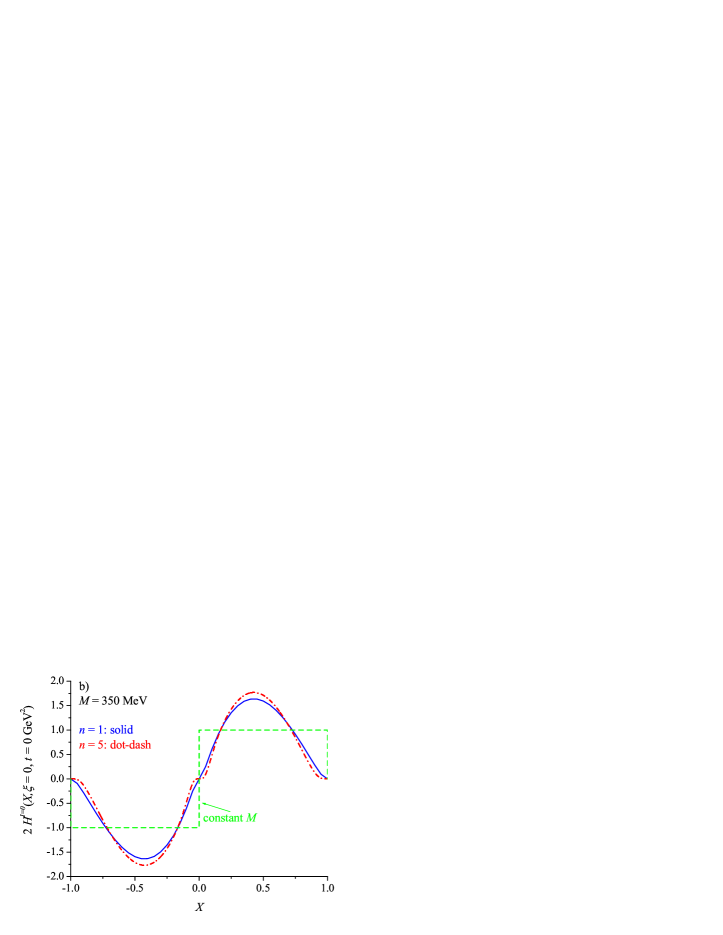
Figure 8: Isoscalar pion SPD, $H^{I=0}(X,\xi,t)$, in the chiral limit ($m_{\pi}=0$) for $M=350$ MeV; for $t=-0.25$ and $0$ GeV² plotted as function of $X$ for fixed $\xi$. In Fig.a) dashed-dotted curve corresponds to diagrams a)+b) of Fig.2, and dashed line to diagram c), whereas the solid curve corresponds to the sum. In the forward case (Fig.b)) we show results for $n=1$ (solid) and 5 (dashed-dotted line), as well as the distribution corresponding to constant $M(k)$ [22]. Note that in Fig.b.) $2H^{I=0}$ for $X<0$ is equal to $-\overline{d}(-X)$ distribution in $\pi^{+}$ while for $X>0$ it corresponds to $u(X)$.

obtained within the instanton models. The experimental value [25] is, however, bigger: $\langle(r_{\pi}^{em})^{2}\rangle=(0.66\mbox{ fm})^{2}$. This can be, however, cured by the pion loops, which are neglected in the present approach.

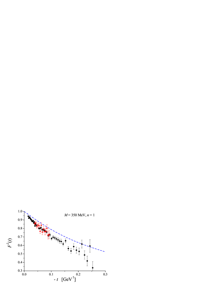
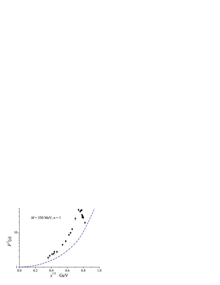
Figure 9: Pion form factors in space like (upper fig.) and time like (lower fig.) regions. Theoretical curves correspond to $M=350$ MeV and $n=1$. Experimental data are taken from: dots [25], triangles [26], squares [27].

5 Soft pion theorems

Soft pion theorems relate 2$\pi$DAs for one pion momentum going to 0 with the one pion light cone distribution amplitude.

We recall the definitions of the axial-vector and pseudo-tensor one pion DAs:

$$\phi_{\pi}^{AV}(u)=\frac{1}{i\sqrt{2}F_{\pi}}\int\limits_{-\infty}^{+\infty}\frac{d\lambda}{\pi}e^{-i\lambda(2u-1)(n\cdot P)}\left\langle 0\right|\bar{d}(\lambda n)\,\hbox to0.0pt{/\hss}n\gamma_{5}\,u(-\lambda n)\left|\pi^{+}(P)\right\rangle$$ (46)

$$\frac{d}{du}\phi_{\pi}^{PT}(u)= -\frac{6F_{\pi}}{i\sqrt{2}\left\langle\bar{q}q\right\rangle}\int\limits_{-\infty}^{+\infty}\frac{d\lambda}{\pi}e^{-i\lambda(2u-1)(n\cdot P)}$$

$$\times\left\langle 0\right|\bar{d}(\lambda n)\,in^{\alpha}P^{\beta}\sigma_{\alpha\beta}\gamma_{5}\,u(-\lambda n)\left|\pi^{+}(P)\right\rangle.$$ (47)

The matrix element entering the definitions (46, 47), calculated in the present model, gives:

$$\left\langle 0\right|\bar{d}(z_{1})\gamma u(z_{2})\left|\pi^{+}(P)\right\rangle=-\frac{\sqrt{2}N_{C}}{F_{\pi}}\int\frac{d^{4}k}{(2\pi)^{4}}e^{i(k-P)z_{1}-ikz_{2}}\,\mathcal{T}(k,k-P),$$ (48)

with

$$\mathcal{T}(k,k-P) =\mbox{Tr}\left(\gamma\frac{\sqrt{M_{k}}}{\hbox to0.0pt{/\hss}k-M_{k}+i\epsilon}\gamma^{5}\frac{\sqrt{M_{k-P}}}{(\hbox to0.0pt{/\hss}k-\hbox to0.0pt{/\hss}P)-M_{k-P}+i\epsilon}\right)$$

$$=\frac{\sqrt{M_{k}M_{k-P}}\,\mbox{Tr}\left(\gamma\gamma^{5}[-\hbox to0.0pt{/\hss}k+M_{k}][(\hbox to0.0pt{/\hss}k-\hbox to0.0pt{/\hss}P)+M_{k-P}]\right)}{\left[k^{2}-M_{k}^{2}+i\epsilon\right]\left[(k-P)^{2}-M_{k-P}^{2}+i\epsilon\right]}$$ (49)

Further calculations require an explicit form of $\gamma$. Substituting (48) into (46) and (47) we get

$$\phi_{\pi}^{AV}(u)=\frac{iN_{C}}{F_{\pi}^{2}}\int\frac{d^{4}k}{(2\pi)^{4}}\delta(n\cdot(k-u\,P))\,\mathcal{T}(k,k-P)|_{\gamma=\hbox to0.0pt{/\hss}n\gamma_{5}}$$ (50)

and

$$\frac{d}{du}\phi(u)=-\frac{6iN_{C}}{\left\langle\bar{q}q\right\rangle}\int\frac{d^{4}k}{(2\pi)^{4}}\delta(n\cdot(k-u\,P))\,\mathcal{T}(k,k-P)|_{\gamma=in^{\alpha}P^{\beta}\sigma_{\alpha\beta}\gamma_{5}}$$ (51)

respectively. Similarly, in the case of $2\pi$DAs, from (5) and (31) we get

$$\Phi_{2\pi}^{I=0}(u,v,s)= \frac{iN_{C}}{F_{\pi}^{2}}\int\frac{d^{4}k}{(2\pi)^{4}}\delta(n\cdot(k-u\,P))$$

$$\left[\mathcal{T}_{1}(k-P,k)+\mathcal{T}_{2}\left(k-P,k-p_{2},k\right)+\mathcal{T}_{2}\left(k-P,k-p_{1},k\right)\right]$$ (52)

and

$$\Phi_{2\pi}^{I=1}(u,v,s)= \frac{iN_{C}}{F_{\pi}^{2}}\int\frac{d^{4}k}{(2\pi)^{4}}\delta(n\cdot(k-u\,P))$$

$$\left[\mathcal{T}_{2}\left(k-P,k-p_{2},k\right)-\mathcal{T}_{2}\left(k-P,k-p_{1},k\right)\right],$$ (53)

with $\mathcal{T}_{1}$ and $\mathcal{T}_{2}$ defined in (33) and (34). Soft pion theorems relate matrix elements (48) and (31) for one pion momentum, say $p_{2}\rightarrow 0$ and for different $\gamma$ and $\Gamma$. For $\mathcal{T}_{1}$ we have:

$$\mathcal{T}_{1}(k-P,k)=\frac{\sqrt{M_{k-P}M_{k}}\;\mbox{Tr}\left(\Gamma\left[(\hbox to0.0pt{/\hss}k-\hbox to0.0pt{/\hss}P)+M_{k-P}\right]\left[\hbox to0.0pt{/\hss}k+M_{k}\right]\right)}{\left[(k-P)^{2}-M_{k-P}^{2}+i\epsilon\right]\left[k^{2}-M_{k}^{2}+i\epsilon\right]},$$ (54)

whereas for the two $\mathcal{T}_{2}$’s in the limit $p_{2}\rightarrow 0$ (that is $v\rightarrow 1$) we get:

$$\mathcal{T}_{2}(k-P,k,k) =-\frac{\sqrt{M_{k-P}M_{k}}M_{k}\;\mbox{Tr}\left(\Gamma\left[\left(\hbox to0.0pt{/\hss}k-\hbox to0.0pt{/\hss}P\right)+M_{k-P}\right]\right)}{\left[(k-P)^{2}-M_{k-P}^{2}+i\epsilon\right]\left[k^{2}-M_{k}^{2}+i\epsilon\right]},$$ (55)

$$\mathcal{T}_{2}(k-P,k-P,k) =-\frac{\sqrt{M_{k-P}M_{k}}M_{k-P}\;\mbox{Tr}\left(\Gamma\left[\hbox to0.0pt{/\hss}k+M_{k}\right]\right)}{\left[(k-P)^{2}-M_{k-P}^{2}+i\epsilon\right]\left[k^{2}-M_{k}^{2}+i\epsilon\right]}.$$ (56)

5.1 Chirally even $2\pi$DA and axial-vector wave function

Consider first the soft pion theorem discussed already at the end of Sect.3.1. To this end let us take

$$\gamma=\hbox to0.0pt{/\hss}n\gamma_{5}.$$ (57)

Then

$$\mathcal{T}(k,k-P)|_{\Gamma=\hbox to0.0pt{/\hss}n\gamma_{5}}=\frac{\sqrt{M_{k}M_{k-P}}\left[-M_{k-P}\,\mbox{Tr}\left(\hbox to0.0pt{/\hss}n\hbox to0.0pt{/\hss}k\right)+M_{k}\;\mbox{Tr}\,\left(\hbox to0.0pt{/\hss}n(\hbox to0.0pt{/\hss}k-\hbox to0.0pt{/\hss}P)\right)\right]}{\left[k^{2}-M_{k}^{2}+i\epsilon\right]\left[(k-P)^{2}-M_{k-P}^{2}+i\epsilon\right]}.$$ (58)

For two pions we have to take

$$\Gamma=\hbox to0.0pt{/\hss}n.$$ (59)

Then in the soft limit $p_{1}=P$, $p_{2}=0$ (this means $v=1$) the isovector combination in Eq.(53) reads

$$\mathcal{T}_{2}(k-P,k,k)|_{\Gamma=\hbox to0.0pt{/\hss}n}-\mathcal{T}_{2}(k-P,k-P,k)|_{\Gamma=\hbox to0.0pt{/\hss}n}$$

$$=-\frac{\sqrt{M_{k-P}M_{k}}\,\left[M_{k}\mbox{Tr}(\hbox to0.0pt{/\hss}n(\hbox to0.0pt{/\hss}k-\hbox to0.0pt{/\hss}P))-M_{k-P}\mbox{Tr}(\hbox to0.0pt{/\hss}n\hbox to0.0pt{/\hss}k)\right]}{\left[(k-P)^{2}-M_{k-P}^{2}+i\epsilon\right]\left[k^{2}-M_{k}^{2}+i\epsilon\right]}$$

$$=-\mathcal{T}(k-P,k)|_{\gamma=\hbox to0.0pt{/\hss}n\gamma_{5}}$$ (60)

Similarly, for the sum entering the isoscalar combination in Eq.(31) we have:

$$\mathcal{T}_{1}(k-P,k)|_{\Gamma=\hbox to0.0pt{/\hss}n}+\mathcal{T}_{2}(k-P,k,k)|_{\Gamma=\hbox to0.0pt{/\hss}n}+\mathcal{T}_{2}(k-P,k-P,k)|_{\Gamma=\hbox to0.0pt{/\hss}n}=0.$$ (61)

Hence the soft pion theorem for the chirally even $2\pi$DA takes the following form

$$\Phi_{2\pi,\,\chi even}^{I=0}(u,v=1,s=0)=0,$$ (62)

$$\Phi_{2\pi,\,\chi even}^{I=1}(u,v=1,s=0)=-\phi_{\pi}^{AV}(u).$$ (63)

5.2 Chirally odd $2\pi$DA and pseudo-tensor wave function

Let us now consider chirally odd $2\pi$DA in the soft pion limit. To this end let us take

$$\gamma=in^{\alpha}P^{\beta}\sigma_{\alpha\beta}\gamma_{5}=\frac{1}{2}\left[\hbox to0.0pt{/\hss}P,\hbox to0.0pt{/\hss}n\right]\gamma_{5}$$ (64)

whose matrix element defines the derivative of pseudo-tensor one pion distribution amplitude. Then

$$\mathcal{T}(k,k-P)|_{\gamma=\frac{1}{2}\left[\hbox to0.0pt{/\hss}P,\hbox to0.0pt{/\hss}n\right]\gamma_{5}}=-\frac{1}{2}\frac{\sqrt{M_{k}M_{k-P}}\,\mbox{Tr}\left[\hbox to0.0pt{/\hss}P,\hbox to0.0pt{/\hss}n\right]\hbox to0.0pt{/\hss}k(\hbox to0.0pt{/\hss}k-\hbox to0.0pt{/\hss}P)}{\left[k^{2}-M_{k}^{2}+i\epsilon\right]\left[(k-P)^{2}-M_{k-P}^{2}+i\epsilon\right]}.$$ (65)

For 2 pions let us take

$$\Gamma=in^{\alpha}P^{\beta}\sigma_{\alpha\beta}=\frac{1}{2}\left[\hbox to0.0pt{/\hss}P,\hbox to0.0pt{/\hss}n\right].$$ (66)

Here only $\mathcal{T}_{1}$ survives

$$\mathcal{T}_{1}(k-P,k)|_{\Gamma=\frac{1}{2}\left[\hbox to0.0pt{/\hss}P,\hbox to0.0pt{/\hss}n\right]} =\frac{1}{2}\frac{\sqrt{M_{k-P}M_{k}}\mbox{Tr}\left(\left[\hbox to0.0pt{/\hss}P,\hbox to0.0pt{/\hss}n\right](\hbox to0.0pt{/\hss}k-\hbox to0.0pt{/\hss}P)\hbox to0.0pt{/\hss}k\right)}{\left[(k-P)^{2}-M_{k-P}^{2}+i\epsilon\right]\left[k^{2}-M_{k}^{2}+i\epsilon\right]}$$

$$=\mathcal{T}(k,k-P)|_{\gamma=\frac{1}{2}\left[\hbox to0.0pt{/\hss}P,\hbox to0.0pt{/\hss}n\right]\gamma_{5}}$$ (67)

while $\mathcal{T}_{2}=0$. Therefore the soft pion theorem relates the isoscalar part of the chirally odd $2\pi$DA to the derivative of pseudo-tensor one pion amplitude:

$$\Phi_{2\pi,\,\chi odd}^{I=0}(u,v=1,s=0)=-\frac{\left\langle\bar{q}q\right\rangle}{6F_{\pi}^{2}}\frac{d}{du}\phi_{\pi}^{PT}(u),$$ (68)

$$\Phi_{2\pi,\,\chi odd}^{I=1}(u,v=1,s=0)=0$$ (69)

This result cannot be derived by current algebra. Since the pseudo-tensor one pion distribution amplitude is close to the asymptotic form $6u(1-u)$ [10] therefore we expect $\Phi_{2\pi,\chi odd}^{I=0}(u,v=0,s=0)\sim 1-2u$. That this is indeed the case can be seen from Fig.6.a. We recall that with our definitions (5) and (7) the chirally odd $2\pi$DAs have the dimension of mass.

6 Pion structure function

As explained in Sect.3.1 skewed pion distributions are in the forward limit directly related to the parton distributions inside the pion. For example, as explained after Eqs.(25,26) and as seen from Fig.8.b

$$u^{\pi^{+}}(x)=\bar{d}^{\pi^{+}}(x)=2H^{I=0}(x,\xi=0,t=0).$$ (70)

On the other hand one can relate pion quark distributions to the wave functions for all Fock states and polarizations [30]. For $\pi^{+}$ we have

$$u^{\pi^{+}}(x) = \sum\limits_{\mbox{Fock states}}\sum\limits_{\lambda}\int\frac{d^{2}k_{T}}{2\left(2\pi\right)^{3}}\,\left|\psi_{\lambda}(x,k_{T})\right|^{2}$$ (71)

$$= \int\frac{d^{2}k_{T}}{2\left(2\pi\right)^{3}}\,\left|\psi^{AV}(x,k_{T})\right|^{2}+\ldots$$

where we have saturated the sum over the different Fock components and polarizations by the axial-vector wave function. The function $\psi^{AV}$ is (for $N_{c}=3$) normalized in the following way [30]:

$$\int\limits_{0}^{1}dx\,\int\frac{d^{2}k_{T}}{\left(2\pi\right)^{3}}\psi^{AV}(x,\vec{k}_{T})=\frac{F_{\pi}}{\sqrt{3}}.$$ (72)

It is clear that the normalization condition for $u^{\pi^{+}}$

$$\int\limits_{0}^{1}dx\,u^{\pi^{+}}(x)=1$$ (73)

and normalization condition (72) are in general incompatible since other components denoted by dots in Eq.(71) are of importance. For example in a model with a constant $M$ one obtains for $\psi^{AV}$ [7]:

$$\psi(u,\vec{k}^{AV}_{T})=\Theta\left(u(1-u)\right)\frac{2\sqrt{3}}{F_{\pi}}\frac{M^{2}}{\vec{k}_{T}^{2}+M^{2}}$$ (74)

and the normalization condition (72) is achieved by imposing a cutoff $\Lambda$ on the transverse momentum integration $dk^{2}_{T}$:

$$F_{\pi}^{2}=\frac{N_{c}M^{2}}{\left(2\pi\right)^{2}}\ln\frac{M^{2}+\Lambda^{2}}{M^{2}}.$$ (75)

It is now straightforward to calculate $u^{\pi^{+}}$

$$u^{\pi^{+}}(x)=\Theta\left(x(1-x)\right)\frac{6}{\left(2\pi\right)^{2}}\frac{M^{2}}{F_{\pi}^{2}}\left[1-\exp\left(-\frac{\left(2\pi\right)^{2}F_{\pi}^{2}}{N_{c}M^{2}}\right)\right].$$ (76)

The normalization constant is, as expected, smaller than 1, however, for $M=350$ MeV we get 0.9 – a fairly satisfactory result for such a simplistic model. Of course the properly defined quark distribution is also properly normalized [21, 22].

In the present model [9]

$$\psi^{AV}(x,\vec{k}_{T})=\frac{2\sqrt{3}M^{2}}{\Lambda^{2}F_{\pi}}\sum\limits_{i,k}f_{i}f_{k}\,\frac{z_{i}^{n}z_{k}^{3n}x+z_{i}^{3n}z_{k}^{n}(1-x)}{\frac{\displaystyle\vec{k}_{T}^{2}}{\displaystyle\Lambda^{2}}+1+z_{i}x+z_{k}(1-x)}$$ (77)

and the normalization condition for $M=350$ MeV and $n=2$ gives $0.88$ instead of $1$. The shape is also different from the properly normalized result obtained with the help of Eq.(70), however, it can be explicitly seen that for large $x$ both definitions converge, as they should [31]. This is depicted in Fig.10.

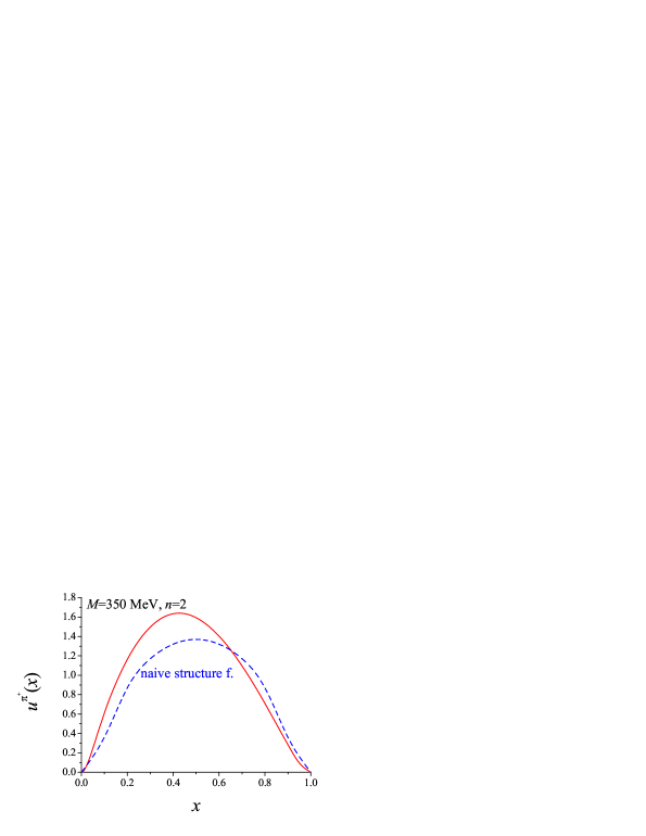
Figure 10: Comparison of the $u$ quark distribution in $\pi^{+}$ defined by Eq.(70) (solid line) and the ”naive” one defined by Eq.(71) (dashed line) for $M=350$ MeV and $n=2$.

One of the major problems of the effective models like the one considered here, is the normalization scale $Q_{0}$ at which the model is defined. This is crucial shortcoming as far as the comparison with the experimental data is concerned. It is argued that the relevant scale for the instanton motivated models is of the order of the inverse instanton size $1/\rho$ i.e. approximately 600 MeV. The precise definition of $Q_{0}$ is only possible within QCD and in all effective models one can use only qualitative order of magnitude arguments to estimate $Q_{0}$. A more practical way to determine $Q_{0}$ was discussed in Ref.[10] where we associated $Q_{0}$ with the transverse integration cutoff $K_{T}$ which was of the order of $760<K_{T}<1100$ MeV.

On the other hand in Refs.[22] it was argued that the pertinent model scale may be as small as 350 MeV. This estimate is based on the requirement that the total momentum carried by the quarks equals to the one measured experimentally at $Q=4$ GeV², i.e. 47% . In that way the initial evolution scale $Q_{0}$ can be adjusted. It is, however, problematic whether one can use QCD evolution equations at such low $Q_{0}$.

Since, as will be discussed in Sect.7 , our model has problems with the momentum sum rule, therefore we cannot use the above prescription to fix $Q_{0}$. In Figs.11 we simply show the shape of the valence, sea and gluon distributions calculated in the model and evolved (in the leading log approximation) to the scale $Q^{2}=4$ GeV² assuming $Q_{0}=450$ and $350$ MeV. As initial conditions we take valence quark distributions as calculated in the model with sea and gluon distribution equal to zero at the initial scale $Q_{0}$. Therefore both sea quarks and gluons are generated dynamically during the evolution. In Figs.11 we also show ”experimental data” as extracted from the pion-proton Drell-Yan and direct photon production [5, 6]. For comparison we also show results of Ref.[22] with a constant quark distribution at initial scale.

It can be seen from Figs.11 that our quark distribution differs from the distributions extracted from the data. However, two existing experimental parameterizations are not compatible. Interestingly, the constant initial quark distribution after evolving to $Q^{2}=4$ GeV² fits very well parameterization of Ref.[5]. Unfortunately for the sea, both constant and our distributions do not follow the experimental parameterization. This suggests that rather than compare model results for pion parton distributions with the ones extracted from the data it is perhaps more appropriate to calculate the cross section itself and compare directly with the data.

There have been several other calculations of the pion structure function in the literature. A result similar to ours was obtained in Refs.[32] where the authors calculate explicitly a hand-bag diagram in a local NJL (nonbosonized) model in the Bjorken limit. They, however, introduce an $x$ dependent cutoff in order to regularize the divergent integrals and get proper behavior of the valence quark distribution in the large $x$ limit. Their result is in agreement with a similar calculation of Ref.[33]. In an approach based on Ward-Takahashi identities, which is in fact equivalent to the local NJL model with a sharp momentum cutoff, the valence quark distribution is equal 1 over the whole range of $x$ [22]. This very simple quark distribution is properly normalized, in a sense that the quark number is 1 and its total momentum is 1/2. The vanishing of $q(x)$ for $x\rightarrow 1$ is achieved by DGLAP evolution. We have plotted the result of this evolution in Fig.11.

Direct calculations in the instanton model [34] show phenomenologically quite similar behavior as ours. An advantage of Refs.[34] is that they use well defined currents with nonlocal pieces [35], whereas we use naive quark billinears. This is reflected in wrong normalization of the first moment of the quark distributions which at low scale should be 1 (for $\int dx\,x(u+\overline{d})$ ) as opposed to 0.93 what we get. An even larger mismatch has been reported in a similar model of Ref.[36], where the remainder of the momentum was attributed to gluons and sea, which are, however, absent in our approach.

Our quark distributions show little $n$ dependence. This is depicted in Fig. 12.

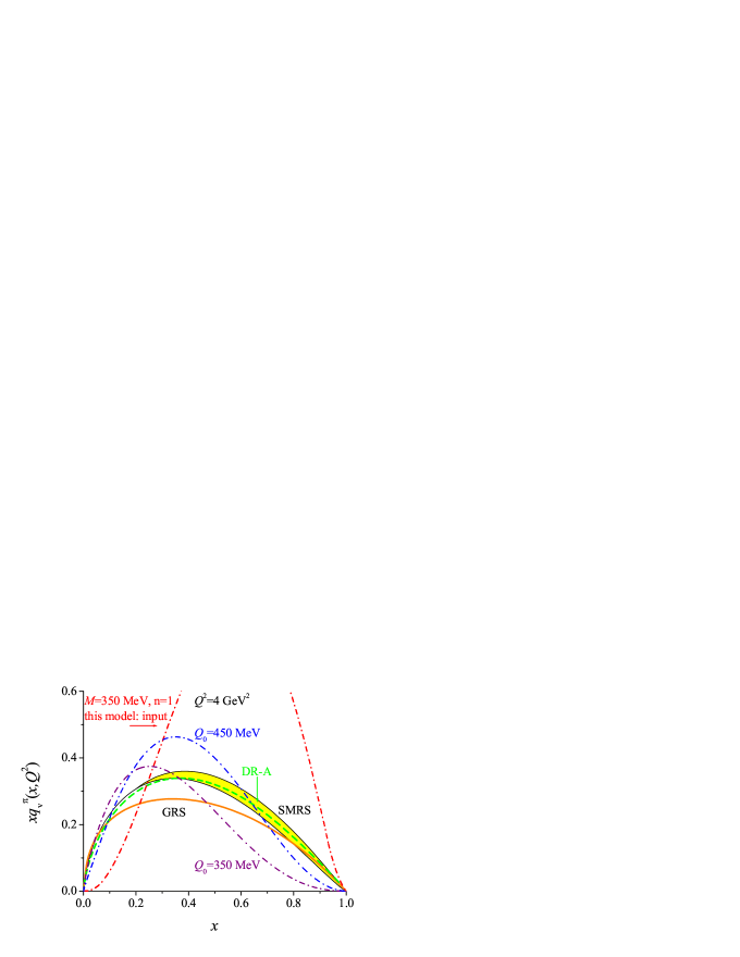
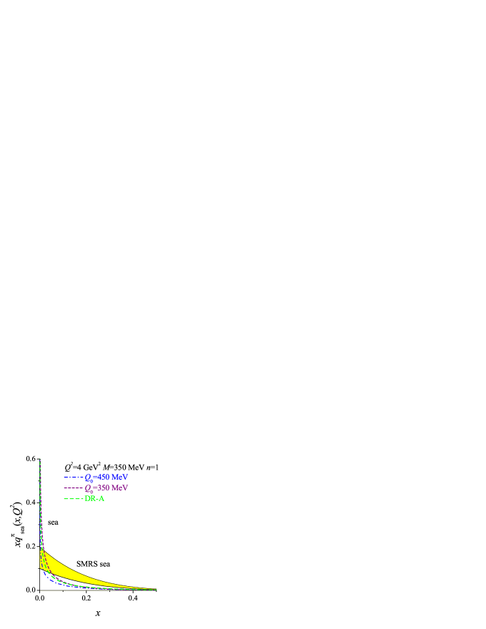
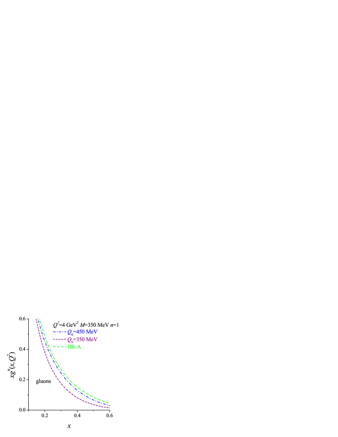
Figure 11: $\pi^{+}$ valence, sea and gluon momentum distributions. Upper panel: input distribution as calculated in the model for $M=350$ MeV and $n=1$ (upper red dashed-dotted curve) and after evolution to $Q^{2}=4$ GeV² from $Q_{0}=450$ MeV (middle blue dashed-dotted curve) and 350 MeV (lower purple dashed-dotted curve). Green dashed line represents constant initial quark distribution [22]. Experimental parameterizations are depicted by a yellow band [5] and orange line [6]. Lower panels: the same for sea quarks and gluons with input distributions equal zero.

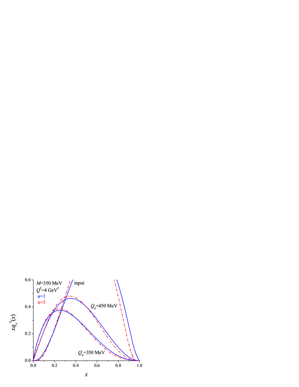
Figure 12: The $n$ dependence of valence quark distributions for $M=350$ MeV and $n=1$ (solid) and 5 (dashed-dotted). Input density corresponds to the model result. Two other sets of curves marked by $Q_{0}=450$ and $Q_{0}=350$ MeV correspond to the distributions evolved to $Q^{2}=4$ GeV² assuming that the model scale was $Q_{0}$.

7 Discussion

In this paper we have calculated the Generalized Distribution Amplitudes using the nonlocal, instanton motivated, chiral quark model. The nonlocality has been taken in the form of Eq.(1) which allowed us to perform all calculations in the Minkowski space. Introducing light cone integration variables allowed us to perform most of the calculations analytically. As a result we were left with the numerical integration in only one variable, $dk_{T}^{2}$.

We define the GDA’s through the matrix elements of the nonlocal quark billinears (5,3.2). Although in QCD this is certainly a correct definition, one might envisage alternative definitions which would be more appropriate for the nonlocal effective models [21, 34]. The reason is that in the limit when the quark operators are taken in the same point, quark billinears (5,3.2) do not correspond to the properly normalized Noether currents. This is because in the nonlocal models Noether currents get additional pieces which restore Ward-Takahashi identities [35]. It is not clear how to generalize quark billinears (5,3.2), since such generalization is, in principle, process dependent. Therefore an alternative way would be to calculate the whole scattering amplitude directly in the effective model and then extract the quantities one is interested in by imposing certain kinematical constraints, like Bjorken limit for example. Although this procedure seems at the first sight attractive, there is a problem because the Bjorken limit requires large momentum transfer, whereas the effective models are defined at low momenta.

In fact the precise determination of the normalization scale $Q_{0}$ at which the model is defined poses a serious problem. In the instanton model of the QCD vacuum [15] that the pertinent energy scale is of the order of the inverse instanton size $Q_{0}=1/\rho\sim 600$ MeV. However, it has been argued in Ref.[22] that $Q_{0}$ may be as low as 350 MeV. This estimate is based on the requirement that the valence quark distribution calculated in the model of Ref.[22] and evolved from $Q_{0}$ to $Q=2$ GeV carry observed fraction of total momentum. Unfortunately we cannot apply the same procedure in our case, since the momentum sum rule is violated in our model. From both equations, (12) and (29) we find the momentum fraction carried by quarks to be 93%, independently of $v$ and $\xi$. This causes the problem, as in the model we use, the pion is built from constituent quarks (there are no gluons) so there is 7% of the pion momentum missing. A natural explanation of this mismatch is that we missed some terms which, in the limit where the quark operators are in the same point, would reduce quark billinears (5,3.2) to the full nonlocal Noether currents [35, 37].

Acknowledgements

We would like to thank W. Broniowski and E. Ruiz-Arriola for comments and discussion. Special thanks are due to K. Goeke and all members of Inst. of Theor. Phys. II at Ruhr-University where part of this work was completed. M.P. acknowledges discussion with S. Brodsky, A. Dorokhov, V.Y. Petrov, P.V. Pobylitsa, M. Polyakov, A. Radyushkin and Ch. Weiss. A.R. acknowledges support of Polish State Committee for Scientific Research under grant 2 P03B 048 22 and M.P. under grant 2 P03B 043 24.

Appendix A Technical details of the calculation of the pion GDAs

Inserting (31) and (32) into (5) and (3.2) respectively we get

$$\Phi_{2\pi}^{I=0}(u,v,s) =\mathcal{J}_{1}(u,v,t)+\mathcal{J}_{2}(u,v,t)+\mathcal{J}_{3}(u,v,t),$$

$$\Phi_{2\pi}^{I=1}(u,v,s) =\mathcal{J}_{2}(u,v,t)-\mathcal{J}_{1}(u,v,t)$$ (78)

and

$$H^{I=0}(X,\xi,t) =\mathcal{I}_{1}(X,\xi,t)+\mathcal{I}_{2}(X,\xi,t)+\mathcal{I}_{3}(X,\xi,t),$$

$$H^{I=1}(X,\xi,t) =\mathcal{I}_{1}(X,\xi,t)-\mathcal{I}_{2}(X,\xi,t).$$ (79)

$\mathcal{J}_{1}$, $\mathcal{J}_{2}$, $\mathcal{J}_{3}$, $\mathcal{I}_{1}$, $\mathcal{I}_{2}$, $\mathcal{I}_{3}$ stand for the integrals:

$$\mathcal{J}_{1}(u,v,s) =\frac{iN_{C}}{2(2\pi)^{4}F_{\pi}^{2}}\left.\int d^{2}k_{\bot}\,\int\limits_{-\infty}^{+\infty}dk_{-}\,\mathcal{T}_{2}(k-P,k-p_{1},k)\right|_{\displaystyle k^{+}=uP^{+}},$$ (80)

$$\mathcal{J}_{2}(u,v,s) =\frac{iN_{C}}{2(2\pi)^{4}F_{\pi}^{2}}\left.\int d^{2}k_{\bot}\,\int\limits_{-\infty}^{+\infty}dk_{-}\,\mathcal{T}_{2}(k-P,k-p_{2},k)\right|_{\displaystyle k^{+}=uP^{+}},$$ (81)

$$\mathcal{J}_{3}(u,v,s) =\frac{iN_{C}}{2(2\pi)^{4}F_{\pi}^{2}}\left.\int d^{2}k_{\bot}\,\int\limits_{-\infty}^{+\infty}dk_{-}\,\mathcal{T}_{1}(k-P,k)\right|_{\displaystyle k^{+}=uP^{+}},$$ (82)

$$\mathcal{I}_{1}(X,\xi,t) =\frac{iN_{C}}{4\left(2\pi\right)^{4}F_{\pi}^{2}}\left.\int d^{2}k_{\bot}\,\int\limits_{-\infty}^{+\infty}dk_{-}\,\mathcal{T}_{2}\left(k-\frac{\Delta}{2},k-\bar{p},k+\frac{\Delta}{2}\right)\right|_{\displaystyle k^{+}=X\bar{p}^{+}},$$ (83)

$$\mathcal{I}_{2}(X,\xi,t) =\frac{iN_{C}}{4\left(2\pi\right)^{4}F_{\pi}^{2}}\left.\int d^{2}k_{\bot}\,\int\limits_{-\infty}^{+\infty}dk_{-}\,\mathcal{T}_{2}\left(k-\frac{\Delta}{2},k+\bar{p},k+\frac{\Delta}{2}\right)\right|_{\displaystyle k^{+}=X\bar{p}^{+}},$$ (84)

$$\mathcal{I}_{3}(X,\xi,t) =\frac{iN_{C}}{4\left(2\pi\right)^{4}F_{\pi}^{2}}\left.\int d^{2}k_{\bot}\,\int\limits_{-\infty}^{+\infty}dk_{-}\,\mathcal{T}_{1}\left(k-\frac{\Delta}{2},k+\frac{\Delta}{2}\right)\right|_{\displaystyle k^{+}=X\bar{p}^{+}},$$ (85)

with $\mathcal{T}_{1}$ and $\mathcal{T}_{2}$ defined in (33, 34). It is convenient to introduce the scaled variables:

$$\kappa^{\mu}=\frac{k^{\mu}}{\Lambda},\qquad\omega^{2}=\frac{s}{\Lambda^{2}},\qquad\vec{\tau}_{\perp}=\frac{\vec{p}_{\perp}}{\Lambda},\qquad\tau=\frac{\tilde{t}}{4\Lambda^{2}},\qquad\vec{\delta}_{\perp}=\frac{\vec{\Delta}_{\perp}}{2\Lambda}$$ (86)

and the notation:

$$\bar{u}=1-u,\qquad\bar{v}=1-v.$$ (87)

We introduce the factors

$$f_{i}=\prod\limits_{{}_{\scriptstyle k\neq i}^{\scriptstyle k=1}}^{4n+1}\frac{1}{z_{i}-z_{k}},$$ (88)

which we will use below. $z_{i}$ are $4n+1$ roots of the Eq. (44). The factors $f_{i}$ have a property:

$$\sum\limits_{i=1}^{4n+1}z_{i}^{m}f_{i}=\left\{\begin{array}[c]{ccc}0&\mbox{for}&m<4n,\\ 1&\mbox{for}&m=4n.\end{array}\right.$$ (89)

This property is crucial for the convergence of the integrals (80-85), in analogy to the case of the pion distribution amplitude [9]. This property is true for any set of different $4n+1$ numbers, irrespectively to the fact that they are solutions of certain polynomial equation.
It can be shown that

$$\mathcal{J}_{3}(u,v,s)=\mathcal{J}_{3}(u,s)=-\mathcal{J}_{3}(\bar{u},s),$$ (90)

$$\mathcal{J}_{1}(\bar{u},v,s)=-\mathcal{J}_{2}(u,v,s),$$ (91)

$$\mathcal{J}_{1}(u,\bar{v},s)=\mathcal{J}_{2}(u,v,s)$$ (92)

and

$$\mathcal{I}_{2}(-X,\xi,t)=-\mathcal{I}_{1}(X,\xi,t),\qquad\mathcal{I}_{3}(-X,\xi,t)=-\mathcal{I}_{3}(X,\xi,t),$$ (93)

$$\mathcal{I}_{2}(X,-\xi,t)=\mathcal{I}_{1}(X,\xi,t),\qquad\mathcal{I}_{3}(X,-\xi,t)=\mathcal{I}_{3}(X,\xi,t).$$ (94)

The properties (90-94), together with Eqs. (A-79), provide the correct symmetry properties for $2\pi$DAs (8, 9) and SPDs (21, 22)
For $\mathcal{J}_{3}(u,s)$ we get analytical results:

$$\mathcal{J}_{3}(u,s)=\frac{N_{C}M^{2}}{\left(2\pi\right)^{2}F_{\pi}^{2}}\sum_{i=1}^{4n+1}\sum_{k=1}^{4n+1}z_{i}^{n}z_{k}^{n}\,f_{i}\,f_{k}\left(uz_{i}^{2n}-\bar{u}z_{k}^{2n}\right)\ln\left(-u\bar{u}\omega^{2}+1+\bar{u}z_{i}+uz_{k}\right).$$ (95)

If $0\leq u\leq\bar{v}$ then $\mathcal{J}_{2}(u,v,s)$ reads

$$\mathcal{J}_{2}(u,v,s)$$

$$=(-1)^{n+1}\frac{iN_{C}M^{2}}{\left(2\pi\right)^{3}F_{\pi}^{2}}\sum_{i=1}^{4n+1}z_{i}^{n}f_{i}\int\limits_{0}^{\infty}d\left(\kappa_{\bot}^{2}\right)\,\frac{u^{7n+1}\left[\left(-u\bar{u}\omega^{2}+\vec{\kappa}_{\perp}^{2}+1+\bar{u}z_{i}\right)\right]^{n}}{\prod\limits_{k=1}^{4n+1}\left(-u\bar{u}\omega^{2}+\vec{\kappa}_{\perp}^{2}+1+\bar{u}z_{i}+uz_{k}\right)}$$

$$\times\int\limits_{C(0,1)}d\lambda\,\frac{\lambda^{4n}}{\prod\limits_{k=1}^{4n+1}\left(A(u)\lambda^{2}+B_{ik}(u,v)\lambda+A(u)\right)}\,g(u,v)$$

$$=: \mathcal{F}(u,v,s),$$ (96)

where

$$g(u,v)=\mu^{2}\left[-\bar{u}\left(\frac{-u\bar{u}\omega^{2}+\vec{\kappa}_{\perp}^{2}+1+\bar{u}z_{i}}{u}\right)^{2n}+uz_{i}^{2n}\right.$$

$$\left.-\left(u-\bar{v}\right)\left(\frac{A(u)\lambda^{2}+b_{i}(u,v)\lambda+A(u)}{\lambda u}\right)^{2n}\right]$$

$$+z_{i}^{2n}\left(\frac{-u\bar{u}\omega^{2}+\vec{\kappa}_{\perp}^{2}+1+\bar{u}z_{i}}{u}\right)^{2n}\left(\frac{A(u)\lambda^{2}+b_{i}(u,v)\lambda+A(u)}{\lambda u}\right)^{2n}$$

$$\times\left[-vu\bar{u}\omega^{2}+\underbrace{\left(u+\bar{u}-v\right)}_{\bar{v}}\kappa_{\bot}^{2}+\bar{u}\left(1+z_{i}\right)+\left(u-\bar{u}\right)\sqrt{\kappa_{\bot}^{2}\tau_{\bot}^{2}}\frac{\lambda^{2}+1}{2\lambda}\right].$$ (97)

If $\bar{v}\leq u\leq 1$, then

$$\mathcal{J}_{2}(u,v,s)=-\mathcal{F}(\bar{u},\bar{v},s),$$ (98)

with $\mathcal{F}(u,v,s)$ defined in (96). The symbols $A(u)$, $b_{i}(u,v)$, $B_{ik}(u,v)$ in Eq. (96, 97) stand for

$$A(u)=u\sqrt{\kappa_{\bot}^{2}\tau_{\bot}^{2}},$$

$$b_{i}(u,v)=u\tau_{\perp}^{2}+uv(u-\bar{v})\omega^{2}+\bar{v}(\vec{\kappa}_{\perp}^{2}+1)-(u-\bar{v})z_{i},$$

$$B_{ik}(u,v)=u\tau_{\perp}^{2}+uv(u-\bar{v})\omega^{2}+\bar{v}(\vec{\kappa}_{\perp}^{2}+1)-(u-\bar{v})z_{i}+uz_{k}.$$

Because $H^{I=0}$ and $H^{I=1}$ are symmetric in $\xi$ we can assume $\xi\geq 0$. Then $\mathcal{I}_{1}(X,\xi,t)$ is nonzero only if $-\xi\leq X\leq 1$. Similarly $\mathcal{I}_{3}(X,\xi,t)$ is nonzero only if $-\xi\leq X\leq\xi$.
For $-\xi\leq X\leq\xi$, $\mathcal{I}_{3}(X,\xi,t)$ and $\mathcal{I}_{1}(X,\xi,t)$ read

$$\mathcal{I}_{3}(X,\xi,t)$$

$$=(-1)^{n}\frac{iN_{C}M^{2}}{2(2\pi)^{3}F_{\pi}^{2}}\int\limits_{0}^{\infty}d\left(\kappa_{\bot}^{2}\right)\,\sum_{i=1}^{4n+1}f_{i}\int\limits_{C(0,1)}d\lambda\,\left[(X+\xi)\lambda\,z_{i}\,\left(A\lambda^{2}+b_{i}\lambda+A\right)\right]^{n}$$

$$\times\frac{(X+\xi)\left[\left(X+\xi\right)\lambda\,z_{i}\right]^{2n}+(X-\xi)\left(A\lambda^{2}+b_{i}\lambda+A\right)^{2n}}{\prod\limits_{k=1}^{4n+1}\left[A\lambda^{2}+B_{ik}\lambda+A\right]},$$ (99)

$$\mathcal{I}_{1}(X,\xi,t)=(-1)^{n}\frac{iN_{C}M^{2}}{2(2\pi)^{3}F_{\pi}^{2}}\int\limits_{0}^{\infty}d\left(\kappa_{\bot}^{2}\right)\,\sum_{i=1}^{4n+1}f_{i}\,$$

$$\times\int\limits_{C(0,1)}d\lambda\frac{[(X+\xi)\lambda]^{7n+1}z_{i}^{n}\left(A\lambda^{2}+b_{i}\lambda+A\right)^{n}}{\prod\limits_{k=1}^{4n+1}\left[\left(A\lambda^{2}+B_{ik}\lambda+A\right)\left(C\lambda^{2}+D_{ik}\lambda+C\right)\right]}\,h_{1}^{(a)}(X,\xi,t),$$

where

$$h_{1}^{(a)}(X,\xi,t)$$

$$=\mu^{2}\left[(X-\xi)\left(\frac{A\lambda^{2}+b_{i}\lambda+A}{(X+\xi)\lambda}\right)^{2n}+(X+\xi)z_{i}^{2n}-(X-1)\left(\frac{C\lambda^{2}+d_{i}\lambda+C}{(X+\xi)\lambda}\right)^{2n}\right]$$

$$+z_{i}^{2n}\left(\frac{A\lambda^{2}+b_{i}\lambda+A}{(X+\xi)\lambda}\right)^{2n}\left(\frac{C\lambda^{2}+d_{i}\lambda+C}{(X+\xi)\lambda}\right)^{2n}$$

$$\times\left[\left(\xi^{2}-X^{2}\right)(1-\xi)\tau+\left(\xi+1\right)\kappa_{\bot}^{2}+X\sqrt{\kappa_{\bot}^{2}\delta_{\bot}^{2}}\frac{\lambda^{2}+1}{\lambda}+\left(\xi-1\right)\delta_{\bot}^{2}+(\xi-X)(1+z_{i})\right].$$

For $\xi\leq X\leq 1$, $\mathcal{I}_{1}(X,\xi,t)$ reads

$$\mathcal{I}_{1}(X,\xi,t)=(-1)^{n+1}\frac{iN_{C}M^{2}}{2(2\pi)^{3}F_{\pi}^{2}}\int\limits_{0}^{\infty}d\left(\kappa_{\bot}^{2}\right)\,\sum_{i=1}^{4n+1}f_{i}$$

$$\times\int\limits_{C(0,1)}d\lambda\frac{[(X-1)\lambda]^{6n+1}\left(C\lambda^{2}+f_{i}\lambda+C\right)^{n}\left(C\lambda^{2}+g_{i}\lambda+C\right)^{n}}{\prod\limits_{k=1}^{4n+1}\left[\left(C\lambda^{2}+F_{ik}\lambda+C\right)\left(C\lambda^{2}+G_{ik}\lambda+C\right)\right]}\,h_{1}^{(b)}(X,\xi,t),$$

where

$$h_{1}^{(b)}(X,\xi,t)$$

$$=\mu^{2}\left[(X-\xi)\left(\frac{C\lambda^{2}+g_{i}\lambda+C}{(X-1)\lambda}\right)^{2n}+(X+\xi)\left(\frac{C\lambda^{2}+f_{i}\lambda+C}{(X-1)\lambda}\right)^{2n}\right.$$

$$\left.-(X-1)z_{i}^{2n}\right]$$

$$+\left(\frac{C\lambda^{2}+f_{i}\lambda+C}{(X-1)\lambda}\right)^{2n}\left(\frac{C\lambda^{2}+g_{i}\lambda+C}{(X-1)\lambda}\right)^{2n}z_{i}^{2n}$$

$$\times\left[\frac{\xi^{2}-1}{X-1}\kappa_{\bot}^{2}+\xi\sqrt{\kappa_{\bot}^{2}\delta_{\bot}^{2}}\frac{\lambda^{2}+1}{\lambda}+\left(X-1\right)\delta_{\bot}^{2}+\frac{\xi^{2}-X^{2}}{X-1}(1+z_{i})\right].$$ (102)

The symbols $A$, $b_{i}$, $B_{ik}$, $C$, $d_{i}$, $D_{ik}$, $f_{i}$, $F_{ik}$, $g_{i}$, $G_{ik}$ in Eqs. (99 - 102) stand for

$$A=2X\sqrt{\kappa_{\bot}^{2}\delta_{\bot}^{2}},$$

$$b_{i}=2\xi\left[\left(X^{2}-\xi^{2}\right)\tau+\kappa_{\bot}^{2}+\delta_{\bot}^{2}+1\right]+(\xi-X)z_{i},$$

$$B_{ik}=2\xi\left[\left(X^{2}-\xi^{2}\right)\tau+\kappa_{\bot}^{2}+\delta_{\bot}^{2}+1\right]+(\xi-X)z_{i}+(\xi+X)z_{k},$$

$$C=(1-X)\sqrt{\kappa_{\bot}^{2}\delta_{\bot}^{2}},$$

$$d_{i}=(X-1)\left[(\xi+X)(1-\xi)\tau+\delta_{\bot}^{2}\right]-(1+\xi)\left(\kappa_{\bot}^{2}+1\right)+(X-1)z_{i},$$

$$D_{ik}=(X-1)\left[(\xi+X)(1-\xi)\tau+\delta_{\bot}^{2}\right]-(1+\xi)\left(\kappa_{\bot}^{2}+1\right)+(X-1)z_{i}-(\xi+X)z_{k},$$

$$f_{i}=(X-1)\left[(\xi+X)(1-\xi)\tau+\delta_{\bot}^{2}\right]-(1+\xi)\left(\kappa_{\bot}^{2}+1\right)-(\xi+X)z_{i},$$

$$F_{ik}=(X-1)\left[(\xi+X)(1-\xi)\tau+\delta_{\bot}^{2}\right]-(1+\xi)\left(\kappa_{\bot}^{2}+1\right)-(\xi+X)z_{i}+(X-1)z_{k},$$

$$g_{i}=(X-1)\left[(\xi-X)(1+\xi)\tau-\delta_{\bot}^{2}\right]+(1-\xi)\left(\kappa_{\bot}^{2}+1\right)-(\xi-X)z_{i},$$

$$G_{ik}=(X-1)\left[(\xi-X)(1+\xi)\tau-\delta_{\bot}^{2}\right]+(1-\xi)\left(\kappa_{\bot}^{2}+1\right)-(\xi-X)z_{i}-(X-1)z_{k}.$$

References

- [1] M. Diehl, T. Gousset, B. Pire and O. Teraev, Phys. Rev. Lett. 81 (1988) 1782 [hep-ph/9805380]. M. Diehl, T. Gousset and B. Pire, Phys. Rev. D62 (2000) 073014 [hep-ph/0003233]; hep-ph/0010182.
- [2] X. Ji Phys. Rev. Lett. 78 (1997) 610 [hep-ph/9603249]; Phys. Rev. D55 (1997) 7117 [hep-ph/9609381]; J. Phys. G24 (1998) 1181 [hep-ph/9807358].
- [3] A.V. Radyushkin Phys. Lett. B380 (1996) 417 [hep-ph/9604317]; Phys. Rev. D56 (1997) 5524 [hep-ph/9704207].
- [4] A.V. Radyushkin Acta Phys. Polon. B30 (1999) 3647 [hep-ph/0011383].
- [5] P.J. Sutton, Alan D. Martin, R.G. Roberts and W.J. Stirling, Phys.Rev. D45 (1992) 2349.
- [6] M. Gluck, E. Reya and I. Schienbein, Eur.Phys.J.C10 (1999) 313 [hep-ph/9903288]; M. Gluck, E. Reya and A. Vogt, Z.Phys. C53 (1992) 651.
- [7] V.Yu. Petrov and P.V. Pobylitsa hep-ph/9712203.
- [8] V.Yu. Petrov, M.V. Polyakov, R. Ruskov, C. Weiss and K. Goeke, Phys. Rev. D59 (1999) 114018 [hep-ph/9807229].
- [9] M. Praszałowicz and A. Rostworowski, Phys.Rev. D64 (2001) 074003 [hep-ph/0105188].
- [10] M. Praszałowicz and A. Rostworowski, Phys.Rev. D66 (2002) 054002 [hep-ph/0111196].
- [11] M.V. Polyakov and Ch. Weiss, Phys.Rev. D59 (1999) 091502 [hep-ph/9806390].
- [12] M.V. Polyakov, Nucl.Phys. B555 (1999) 231 [hep-ph/9809483].
- [13] M.V. Polyakov and Ch. Weiss, Phys.Rev. D60 (1999) 114017 [hep-ph/9902451].
- [14] C.E.I. Carneiro and N.A. McDougall, Nucl. Phys. B245 (1984) 293-312
- [15] D.I. Diakonov and V.Yu. Petrov, Nucl. Phys. B245 (1984) 259-292; B272 (1986) 457.
- [16] M. Praszałowicz and A. Rostworowski, talk at 37th Rencontres de Moriond, QCD and Hadronic Interactions, Les Arcs, France, March 16-23, 2002, hep-ph/0205177.
- [17] M. Praszałowicz in: M.J. Amarian et al., Workshop on Spontaneously broken chiral symmetry and hard QCD phenomena, Bad Honnef, Germany, July 15-17, 2002, hep-ph/0211291.
- [18] G.P. Lepage and S.J. Brodsky, Phys. Lett. B87 (1979) 359; Phys. Rev. Lett. 43 (1979) 545; ibid. 43 (1979) 1625 (E); Phys. Rev. D22 (1980) 2157; Phys. Rev. D24 (1981) 1808-1831.
- [19] A.V. Efremov and A.V. Radyushkin, Phys. Lett. B94 (1980) 245; Teor. Mat. Fiz. 44 (1980) 157-171, Theor. Math. Phys. 44 (1981) 664.
- [20] M.A. Shifman and M.I. Vysotsky, Nucl.Phys. B186 (1981) 475.
- [21] E. Ruiz Arriola, lectures at 42nd Cracow School of Theoretical Physics, Flavor Dynamics, Zakopane, Poland, 31 May - 9 June 2002, Acta Phys.Polon. B33 (2002) 4443 [hep-ph/0210007] and references therein.
- [22] E. Ruiz Arriola and W. Broniowski, Phys.Rev.D66 (2002) 094016 [hep-ph/0207266]; R.M. Davidson and E. Ruiz Arriola, Acta Phys.Polon. B33 (2002) 1791 [hep-ph/0110291]; Phys.Lett.B348 (1995) 163.
- [23] A. V. Radyushkin, Phys. Rev. D 58 (1998) 114008 [hep-ph/9803316 ].
- [24] A.P. Bakulev, R. Ruskov, K. Goeke and N.G. Stefanis Phys. Rev. D62 (2000) 054018 [hep-ph/0004111].
- [25] S.R. Amendolia et al. (NA7 Coll.) Nucl. Phys. B277 (1986) 168.
- [26] E.B. Dally et al., Phys. Rev. Lett. 48 (1982) 375; Phys.Rev. D24 (1981) 1718.
- [27] L.M. Barkov et al., Nucl. Phys. 256B (1985) 365.
- [28] M. Praszałowicz and G. Valencia, Nucl.Phys. B341 (1990) 27.
- [29] A.P. Bakulev, A.V. Radyushkin and N.G. Stefanis, Phys. Rev. D62 (2000) 113001 [hep-ph/0005085].
- [30] S.J. Brodsky and G.P. Lepage, in: Perturbative Quantum Chromodynamics A.H. Mueller (Ed.) Adv.Ser.Direct.High Energy Phys. 5 (1989) 93.
- [31] R. Jakob, P. Kroll and M. Raulfs, J.Phys. G22 (1996) 45 [hep-ph/9410304].
- [32] T. Shigetani, K. Suzuki and H. Toki, Phys. Lett. B308 (1993) 383 [hep-ph/9402286]; Nucl. Phys. A579 (1994) 413 [hep-ph/9402277].
- [33] T. Heinzl, Ligh-Cone Quantization: Foundations and Applications, hep-th/0008096 and Nucl. Phys. Proc. Suppl. 90 (2000) 83 [hep-ph/0008314].
- [34] A.E. Dorokhov and L. Tomio, Phys.Rev. D62 (2000) 014016.
- [35] R.D. Bowler and M.C. Birse, Nucl.Phys. A582 (1995) 655 [hep-ph/9407336].
- [36] M.B. Hecht, C.D. Roberts and S.M. Schmidt, Phys.Rev.C63 (2001) 025213 [nucl-th/0008049].
- [37] W. Broniowski, B. Golli and G. Ripka, Nucl.Phys. A703 (2002) 667 [hep-ph/0107139].