$e^{+}e^{-}\to\nu\overline{\nu}A^{0}$ in the two-Higgs-doublet model

Abstract

We compute the cross section for $e^{+}e^{-}\rightarrow{\nu}\overline{\nu}A^{0}$ in the general CP-conserving type-II two-Higgs-doublet model. We sum the contributions from the “$t$-channel” $e^{+}e^{-}\to\nu\overline{\nu}WW\to\nu\overline{\nu}A^{0}$ graphs and “$s$-channel” $e^{+}e^{-}\to ZA^{0}\to\nu\overline{\nu}A^{0}$ graphs, including their interference. Higgs-triangle graphs and all box diagrams are included. For many parameter choices, especially those in the decoupling region of parameter space (light $h^{0}$ and $m_{A^{0}},m_{H^{0}},m_{H^{\pm}}>2m_{Z}$) the Higgs-triangle and box diagrams are found to be of minor importance, the main contributing loops being the top and bottom quark triangle diagrams. The predicted cross section is rather small for $\tan\beta>2$ and/or $m_{A^{0}}>2m_{t}$. However, we also show that if parameters are chosen corresponding to large Higgs self-couplings then the Higgs-triangle graphs can greatly enhance the cross section. We also demonstrate that the SUSY-loop corrections to the $b\overline{b}A^{0}$ coupling could be such as to greatly enhance this coupling, resulting in an enhanced $\nu\overline{\nu}A^{0}$ cross section. Complete cross section expressions are given in the Appendices.

I Introduction

The Higgs mechanism provides an elegant way to explain electroweak symmetry breaking (EWSB) and the origin of the masses of all the observed Standard Model (SM) particles. In many approaches, the symmetry breaking arises from a sector involving scalar fields and leaves behind one or more physical Higgs bosons. Detecting and studying all such Higgs bosons is one of the major objectives of current and future particle physics experiments. The minimal SM contains one ${\rm SU(2)}_{\rm L}$-doublet Higgs field, leading to a single physical CP-even Higgs boson after EWSB. However, the electroweak scale is not stable with respect to radiative corrections in the minimal SM. Numerous extensions of the SM have been proposed to cure this naturalness/hierarchy problem, many of which predict a low-energy effective theory with a Higgs sector that contains two (or more) Higgs doublet fields. Our focus here will be on a general two-Higgs-doublet model (2HDM) (for a review and references see HHG ). In particular, the most promising extension of the SM that resolves the naturalness and hierarchy problems is low-energy supersymmetry (SUSY), which must contain at least two Higgs doublets. For precise gauge-coupling unification, exactly two doublets are preferred, as incorporated in the minimal supersymmetric Standard Model (MSSM). The two-doublet Higgs sector of the MSSM is predicted to be CP-conserving at tree level and to have type-II fermionic couplings in which one doublet ($\Phi_{1}$) gives mass to down-type quarks and charged leptons while the other doublet ($\Phi_{2}$) gives mass to up-type quarks. In this case there are five physical Higgs bosons: the CP-even $h^{0}$ and $H^{0}$, the CP-odd $A^{0}$, and the charged pair $H^{\pm}$. The most important additional parameters of the CP-conserving type-II 2HDM are: (i) $\tan\beta$ ($\tan\beta\equiv v_{2}/v_{1}=\langle\Phi_{2}^{0}\rangle/\langle\Phi_{1}^{0}\rangle$, the ratio of the vacuum expectation values of the neutral members of the two Higgs doublets); and (ii) the mixing angle $\alpha$ that diagonalizes the neutral CP-even Higgs sector.

Higgs searches at the CERN LEP II collider have excluded a SM Higgs boson with mass below 114.4 GeV lep at 95% confidence level. In the context of specific choices for the soft-SUSY-breaking parameters at the TeV scale, LEP II can be used to exclude a range of MSSM Higgs masses and $\tan\beta$. For example, assuming the maximal-top-squark-mixing scenario with $m_{\rm SUSY}=1~{}{\rm TeV}$, LEP II excludes $m_{h^{0}}<91.0$ GeV, $m_{A^{0}}<91.9$ GeV and $0.5<\tan\beta<2.4$ at 95% Confidence Level (CL) lepa ; lep2 . Searches for top quark decay $t\to H^{+}b$ at the Fermilab Tevatron exclude $\tan\beta>50$ when $m_{t}>m_{H^{\pm}}$, and searches for the final state $b\overline{b}h^{0}\to b\overline{b}b\overline{b}$ exclude very high values of $\tan\beta$ as a function of the $h^{0}$ mass tevsum . Precision electroweak measurements provide only weak constraints on $\tan\beta$ yamada . Finally, limits can be placed on $\tan\beta$ as a function of $m_{H^{\pm}}$ based on $\pi^{+},K^{+},B^{+}\to\mu^{+}\nu$ decays and on $K$-$\overline{K}$ and $B$-$\overline{B}$ mixing Marin:2002 . In the context of a type-II model, as defined earlier, these roughly require $1<\tan\beta<200$ for $m_{H^{\pm}}\sim 300~{}{\rm GeV}$. However, much of the MSSM parameter space remains to be explored at future collider experiments. Indeed, for the most general MSSM boundary conditions, there is no lower bound on $\tan\beta$ from LEP II data. For the most general 2HDM, only the presence of two simultaneously light Higgs bosons can be excluded Grzadkowski:1999ye ; opal2hdm .

At Run II of the Tevatron, discovery of the light CP-even Higgs boson $h^{0}$ of the MSSM at the $5\sigma$ level is possible for $m_{h^{0}}\mathrel{\raise 1.29167pt\hbox{$<$\kern-7.5pt\lower 4.30554pt\hbox{$\sim$}}}120$ GeV with 15 ${\rm fb}^{-1}$ of integrated luminosity tev . At the CERN Large Hadron Collider (LHC), discovery of $h^{0}$ is virtually guaranteed over all of the MSSM parameter space lhcATLAS ; lhcCMS ; perini , and measurements of ratios of the the $h^{0}$ partial decay widths in the more prominent decay channels will be possible with precisions on the order of $15\%$ Zeppenfeld . A linear $e^{+}e^{-}$ collider could make precision measurements of the $h^{0}$ couplings with accuracies of a few percent hLCmeas ; TeslaTDR ; Orangebook . In fact, at a linear collider with $\sqrt{s}\geq 350~{}{\rm GeV}$, at least one of the CP-even Higgs bosons of a general 2HDM (or more complicated Higgs sector) is guaranteed to be detected Espinosa:1998xj in the $Zh$ production mode. In contrast, even in the simple 2HDM there is no guarantee that the CP-odd $A^{0}$ can be detected, and the situation only worsens for more complicated Higgs sectors. Thus, it behooves us to explore every option for $A^{0}$ production.

For a CP-conserving Higgs sector, production of a single $A^{0}$ via loop-induced processes could prove critical to a full exploration of the Higgs sector. This is because the most useful tree-level mechanisms for single Higgs production rely on a substantial Higgs coupling to $ZZ$ or $WW$ pairs. Such couplings are absent at tree-level for the purely CP-odd $A^{0}$. If the Higgs sector is CP-violating, then the neutral Higgs bosons will mix with one another and, in general, all will have substantial tree-level $ZZ$ and $WW$ couplings. As a result, in the case of a CP-violating Higgs sector, loop-induced $A^{0}$ production mechanisms would probably not be very important. Thus, loop-induced $A^{0}$ production is mainly of interest for a CP-conserving Higgs sector. We note that there are substantial phenomenological reasons for believing that the Higgs sector will prove to be CP-conserving. In particular, CP-conservation is the most straightforward approach to avoiding conflict with the constraints coming from the anomalous magnetic moment of the muon $(g_{\mu}-2)$ Bennett:2002jb and the non-observation of electric dipole moments (EDMs). Still, we must note that even in the MSSM context substantial CP violation could be introduced at the loop level if the soft-SUSY-breaking parameters have phases, and that a CP-violating Higgs sector can be consistent with the EDM and $(g_{\mu}-2)$ constraints if there are carefully orchestrated cancellations between CP-violating contributions to these observables cpcancellations .

Let us review in detail the difficulties associated with producing and detecting a purely CP-odd $A^{0}$. At a hadron collider, the absence of tree-level $ZZA^{0}$ and $WWA^{0}$ couplings implies that: (i) the $W^{*}\to WA^{0}$ production mode is suppressed, as particularly relevant at the Tevatron; (ii) the $gg\to A^{0}\to WW$ and $gg\to A^{0}\to ZZ$ production/decay modes (the “gold-plated” processes for discovery of a heavy SM-like Higgs boson) have very low rates because the branching fractions $B(A^{0}\to ZZ)$ and $B(A^{0}\to WW)$ are small; and (iii) at the LHC, the $gg\to A^{0}\to\gamma\gamma$ rate is numerically small. With regard to the latter, we note that had $\Gamma(A^{0}\to\gamma\gamma)$ been of SM-like size, the absence of tree-level $A^{0}\to WW,ZZ$ decays would have implied substantial $B(A^{0}\to\gamma\gamma)$ and a useful $gg\to A^{0}\to\gamma\gamma$ rate even for large $m_{A^{0}}$. However, the absence of the $W$-loop (the largest contribution in the case of a SM-like Higgs) results in an even greater suppression of $\Gamma(A^{0}\to\gamma\gamma)$ than of $\Gamma_{A^{0}}^{\rm tot}$. At an $e^{+}e^{-}$ collider, the $e^{+}e^{-}\to Z^{*}\to ZA^{0}$ and $e^{+}e^{-}\to\nu\overline{\nu}W^{*}W^{*}\to\nu\overline{\nu}A^{0}$ processes are only present at the one-loop level.

In general, the $A^{0}$ can be pair produced at tree-level. However, the rates for Higgs pair production are generally too small for observation at the Tevatron and LHC since they are electroweak in strength and must compete against enormous QCD backgrounds. Pair production is, however, potentially useful at a $e^{+}e^{-}$ machine. Such processes include $e^{+}e^{-}\to Z^{*}\to ZA^{0}A^{0}$ zzaa ; Farris:2002ny , $e^{+}e^{-}\to\nu\overline{\nu}W^{*}W^{*}\to\nu\overline{\nu}A^{0}A^{0}$ wwaa ; Farris:2002ny and $e^{+}e^{-}\to Z^{*}\to H^{0}A^{0}$ or $h^{0}A^{0}$ (see HHG ). However, all of these processes can be simultaneously suppressed by kinematics and/or small couplings. In particular, this occurs in the decoupling limit of a 2HDM that typically arises when $m_{A^{0}}>2m_{Z}$ Gunion:2002zf . In the decoupling limit $m_{H^{0}}\sim m_{A^{0}}\gg m_{h^{0}}$, implying that $\sqrt{s}>2m_{A^{0}}$ is required for $H^{0}A^{0}$, $ZA^{0}A^{0}$ and $\nu\overline{\nu}A^{0}A^{0}$ production (all of which would otherwise have large cross sections since the $ZZA^{0}A^{0}$ and $WWA^{0}A^{0}$ couplings are fixed by the standard quadratic gauge couplings of the $A^{0}$ and the $ZH^{0}A^{0}$ coupling is maximal in this limit), while $h^{0}A^{0}$ production is strongly suppressed in the decoupling limit by a factor of order $m_{Z}^{4}/m_{A^{0}}^{4}$ in the square of the $h^{0}A^{0}Z$ coupling. This decoupling limit is automatic in the context of the MSSM and is quite natural in the case of a more general 2HDM. In the general 2HDM there are other scenarios not related to this standard decoupling limit in which detection of the $A^{0}$ on its own would also be critical. In particular, it is possible to choose Higgs sector parameters in such a way that the $A^{0}$ is the only light Higgs boson while maintaining consistency with precision electroweak measurements Chankowski:2000an (see also Gunion:2002zf ). Further, it is possible that a light $A^{0}$ could explain part of the observed discrepancy between the SM prediction for $(g_{\mu}-2)$ and the experimentally measured value Cheung:2001hz . For all the above reasons, it is important to assess more carefully the various possible mechanisms for single $A^{0}$ production.

Consider first the tree-level processes for single $A^{0}$ production. At both the LHC and at an $e^{+}e^{-}$ collider, the only relevant tree-level processes for single $A^{0}$ production are $t\overline{t}A^{0}$ and $b\overline{b}A^{0}$ production. At the LHC, it has long been established that these do not yield an observable signal in a wedge-shaped region of the $(m_{A^{0}},\tan\beta)$ parameter space. This wedge spans a range of moderate $\tan\beta$ values for $m_{A^{0}}>200~{}{\rm GeV}$ and becomes increasingly broad as $m_{A^{0}}$ increases (see, for example, the ATLAS and CMS TDRs lhcATLAS ; lhcCMS ). At an $e^{+}e^{-}$ collider, this wedge is even larger, beginning at a relatively low value of $m_{A^{0}}$ (the precise value depends on the $\sqrt{s}$ of the machine) Djouadi:gp ; Grzadkowski:1999ye ; Grzadkowski:2000wj (see also bbtta3 ; bbtta4 ). In particular, for $m_{A^{0}}+2m_{t}>\sqrt{s}$ (and if Higgs pair production processes are suppressed or kinematically forbidden) there is no known means for detecting the $A^{0}$ using tree-level production mechanisms when $\tan\beta$ is not large enough for the $b\overline{b}A^{0}$ process to have an observable rate. In this situation, we must turn to loop-induced $A^{0}$ production mechanisms.

One possibility is to build a photon collider at the $e^{+}e^{-}$ collider and look for $\gamma\gamma\to A^{0}$ via $t$, $b$ and charged Higgs loops Gunion:1992ce ; Asner:2001ia ; Muhlleitner:2001kw . In particular, the recent realistic study of Ref. Asner:2001ia found that three years of running at a 630 GeV $e^{+}e^{-}$ LC in the photon collider mode could provide a 4$\sigma$ signal for a significant fraction of the $(m_{A^{0}},\tan\beta)$ LHC wedge region with $m_{A^{0}}\leq 500~{}{\rm GeV}$. If $m_{A^{0}}$ could be roughly guessed, e.g., based on the precise measurements of deviations of the $h^{0}$ couplings from their SM values Battaglia:2000jb ; Carena:2001bg ; TeslaTDR ; Kiyoura:2001kj ; ACFA obtainable at a linear $e^{+}e^{-}$ collider, then the energy of the photon collider could be chosen to optimize the $A^{0}$ production cross section resulting in a faster discovery. One-loop production possibilities in $e^{+}e^{-}$ collisions include $e^{+}e^{-}\to\gamma A^{0}$, $e^{+}e^{-}\to Z^{*}\to ZA^{0}$ and $e^{+}e^{-}\to\nu\overline{\nu}A^{0}$ via $WW$ fusion. (The latter two interfere since $Z\to\nu\overline{\nu}$.) The $e^{+}e^{-}\to\gamma A^{0}$ process has been computed in Refs. Djouadi:1996ws ; Akeroyd:1999gu . Results for the $ZA^{0}$ final state (computed assuming the absence of supersymmetric particle loops) appear in Refs. Akeroyd:1999gu ; Farris:2002ny . The possible enhancement of the $ZA^{0}$ rate when SUSY particles are present is discussed in eeZAMSSM .

In this paper, we give a complete calculation of the $W$ boson fusion process $e^{+}e^{-}\to\nu\overline{\nu}W^{*}W^{*}\to\nu\overline{\nu}A^{0}$ in the general CP-conserving 2HDM, which first occurs at one-loop since there is no tree level $W^{+}W^{-}A^{0}$ coupling. We include the process $e^{+}e^{-}\to Z^{*}\to ZA^{0}\to\nu\overline{\nu}A^{0}$ (first computed in Ref. Akeroyd:1999gu ), which leads to the same final state and thus interferes with the $W$ boson fusion process. The process $e^{+}e^{-}\to\nu\bar{\nu}A^{0}$ has also been computed recently in Ref. Arhrib:2002ti . After a review of the structure of the general 2HDM in Sec. II, we present the relevant Feynman diagrams and formulae involved in our calculations in Sec. III. We present numerical results in Sec. IV.

In Sec. IV.1, we employ the tree-level MSSM two-doublet sector (see HHG ) as a benchmark for our study. The Higgs sector of the MSSM is a type-II 2HDM in which the quartic couplings of the two Higgs doublet fields are fixed at tree level by the gauge couplings. In this case, all Higgs sector parameters are determined by just the two parameters $m_{A^{0}}$ and $\tan\beta$, and for $m_{A^{0}}>m_{Z}$ the 2HDM quickly approaches the decoupling limit, described earlier, in which all Higgs self-couplings are small. We compare the full 2HDM results including the loop contributions from quarks, Higgs and gauge bosons with those obtained by including only the top and bottom quark loops, as computed in Farris:2002ny . We show that the $e^{+}e^{-}\to\nu\overline{\nu}A^{0}$ process could provide a viable $A^{0}$ signal for $\tan\beta<1$, thus covering part of the region where $A^{0}$ discovery using tree-level processes is not possible. Further, for such $\tan\beta$ values the $\nu\overline{\nu}A^{0}$ rate would provide a very sensitive measurement of $\tan\beta$. In contrast to the above, the $\nu\overline{\nu}A^{0}$ cross section is typically quite small for $\tan\beta\geq 2$ for parameter choices based on the tree-level MSSM Higgs sector potential. Of course, in the full MSSM, radiative corrections to the tree-level masses should be incorporated as should the contributions with superparticles running in the loop. However, the sparticle loops are in general suppressed by the heavy sparticle masses. A full study of the MSSM, including all the superparticle loop contributions and radiative corrections to the Higgs potential, will appear in nunuafull .

Sec. IV.2 focuses on the general 2HDM with Higgs potential parameters outside the decoupling regime. We find that if the Higgs self-couplings are large (as possible when 2HDM parameters are chosen to lie in a non-decoupling regime) then the $\nu\overline{\nu}A^{0}$ cross section can be greatly enhanced by Higgs triangle diagrams even for such large $h^{0},H^{0},H^{\pm}$ masses that none of these latter Higgs bosons could be directly observed. Indeed, for lower $m_{A^{0}}$ values ($m_{A^{0}}<2m_{t}$), the rate is sufficiently enhanced when $\tan\beta>10$ that the $\nu\overline{\nu}A^{0}$ events could have a detectable rate and provide direct evidence for the large Higgs self-couplings. This probe of the Higgs self-couplings would be especially powerful if some of the other Higgs bosons have themselves been directly observed.

In Sec. IV.3, we illustrate one unusual possibility in the full MSSM context, namely that the $b\overline{b}A^{0}$ coupling could be greatly enhanced by non-decoupling SUSY particle loops, resulting in a huge enhancement for the $e^{+}e^{-}\to\nu\overline{\nu}A^{0}$ cross section.

Finally, Sec. V is reserved for our conclusions. In the Appendices, we collect the complete matrix elements for the various Feynman diagram contributions.

II The CP-conserving 2HDM

We adopt the conventions of Gunion:2002zf for the 2HDM. Let $\Phi_{1}$ and $\Phi_{2}$ denote two complex SU(2)_L-doublet scalar fields with hypercharge $Y=1$. The most general gauge invariant scalar potential is given by

$$\mathcal{V} = m_{11}^{2}\Phi_{1}^{\dagger}\Phi_{1}+m_{22}^{2}\Phi_{2}^{\dagger}\Phi_{2}-[m_{12}^{2}\Phi_{1}^{\dagger}\Phi_{2}+{\rm h.c.}]+{\textstyle{1\over 2}}\lambda_{1}(\Phi_{1}^{\dagger}\Phi_{1})^{2}+{\textstyle{1\over 2}}\lambda_{2}(\Phi_{2}^{\dagger}\Phi_{2})^{2}+\lambda_{3}(\Phi_{1}^{\dagger}\Phi_{1})(\Phi_{2}^{\dagger}\Phi_{2})+\lambda_{4}(\Phi_{1}^{\dagger}\Phi_{2})(\Phi_{2}^{\dagger}\Phi_{1})$$ (1)

$$\quad+\left\{{\textstyle{1\over 2}}\lambda_{5}(\Phi_{1}^{\dagger}\Phi_{2})^{2}+\big{[}\lambda_{6}(\Phi_{1}^{\dagger}\Phi_{1})+\lambda_{7}(\Phi_{2}^{\dagger}\Phi_{2})\big{]}\Phi_{1}^{\dagger}\Phi_{2}+{\rm h.c.}\right\}\,.$$

The terms proportional to $\lambda_{6}$ and $\lambda_{7}$ lead to flavor-changing neutral current interactions (FCNCs) and will be set to zero. This can be achieved by imposing a discrete symmetry $\Phi_{1}\rightarrow-\Phi_{1}$ on ${\cal V}$. However, we allow for a soft (dimension-two) breaking of this symmetry through $m_{12}^{2}\neq 0$. If $\lambda_{6}=\lambda_{7}=0$ but $m_{12}^{2}\neq 0$, the soft breaking of the discrete symmetry generates finite Higgs-mediated FCNCs at one loop. The tree-level supersymmetric form of ${\cal V}$ is obtained from Eq. (1) by the substitutions:

$$\lambda_{1}=\lambda_{2}={\textstyle{1\over 4}}(g^{2}+g^{\prime 2})\,,\quad\lambda_{3}={\textstyle{1\over 4}}(g^{2}-g^{\prime 2})\,,\quad\lambda_{4}=-{\textstyle{1\over 2}}g^{2}\,,\quad\lambda_{5}=\lambda_{6}=\lambda_{7}=0\,,$$ (2)

where $g$ and $g^{\prime}$ are the ${\rm SU(2)}_{L}$ and ${\rm U(1)}_{Y}$ gauge couplings, respectively. In general, $m_{12}^{2}$ and $\lambda_{5}$ (and, if present, $\lambda_{6}$ and $\lambda_{7}$) can be complex. However, we explicitly exclude such CP-violating phases by choosing all coefficients in Eq. (1) to be real and such that spontaneous CP violation is absent. For details, see Ref. Gunion:2002zf . The scalar fields will develop non-zero vacuum expectation values if the mass matrix has at least one negative eigenvalue. Imposing CP invariance and U(1)_EM gauge symmetry, the minimum of the potential corresponds to the following vacuum expectation values:

$$\langle\Phi_{1}\rangle={1\over\sqrt{2}}\left(\begin{array}[]{c}0\\ v_{1}\end{array}\right),\qquad\langle\Phi_{2}\rangle={1\over\sqrt{2}}\left(\begin{array}[]{c}0\\ v_{2}\end{array}\right)\,,$$ (3)

where $v_{i}$ are real in the absence of explicit and spontaneous CP violation. The minimization conditions on the potential can then be used to determine $m_{11}^{2}$ and $m_{22}^{2}$ in terms of the other parameters (with $\lambda_{6}=\lambda_{7}=0$):

$$m_{11}^{2}=m_{12}^{2}t_{\beta}-{\textstyle{1\over 2}}v^{2}\left[\lambda_{1}c_{\beta}^{2}+\lambda_{345}s_{\beta}^{2}\right]\,,\quad m_{22}^{2}=m_{12}^{2}t_{\beta}^{-1}-{\textstyle{1\over 2}}v^{2}\left[\lambda_{2}s_{\beta}^{2}+\lambda_{345}c_{\beta}^{2}\right]\,,$$ (4)

where we have defined:

$$\lambda_{345}\equiv\lambda_{3}+\lambda_{4}+\lambda_{5}\,,\qquad\qquad t_{\beta}\equiv\tan\beta\equiv{v_{2}\over v_{1}}\,,$$ (5)

and $v^{2}\equiv v_{1}^{2}+v_{2}^{2}=4m_{W}^{2}/g^{2}=(246~{}{\rm GeV})^{2}\,.$ It is always possible to choose the phases of the Higgs doublet fields such that both $v_{1}$ and $v_{2}$ are positive, implying that we can take $0\leq\beta\leq\pi/2$. With $\lambda_{6}=\lambda_{7}=0$, all but one of the eight free parameters in Eq. (1) can be fixed after EWSB in terms of $v$, $\tan\beta$, the four physical Higgs masses, and the mixing angle $\alpha$ required to diagonalize the neutral CP-even Higgs sector. In our numerical analysis below, we use the parameter set $m_{A^{0}}$, $m_{H^{0}}$, $m_{h^{0}}$, $m_{H^{\pm}}$, $\alpha$, $\tan\beta$ and $\lambda_{5}$. ($v$ is of course fixed by the measured values of $m_{W}$ and $g$.) The relations (D.20)–(D.23) of Gunion:2002zf with $\lambda_{6}=\lambda_{7}=0$ then give the other $\lambda_{i}$ as:

$$\lambda_{1} = {m_{H^{0}}^{2}c_{\alpha}^{2}+m_{h^{0}}^{2}s_{\alpha}^{2}-m_{A^{0}}^{2}s_{\beta}^{2}\over v^{2}c_{\beta}^{2}}-\lambda_{5}t_{\beta}^{2}\,;$$ (6)

$$\lambda_{2} = {m_{H^{0}}^{2}s_{\alpha}^{2}+m_{h^{0}}^{2}c_{\alpha}^{2}-m_{A^{0}}^{2}c_{\beta}^{2}\over v^{2}s_{\beta}^{2}}-\lambda_{5}t_{\beta}^{-2}\,;$$ (7)

$$\lambda_{3} = {(m_{H^{0}}^{2}-m_{h^{0}}^{2})s_{\alpha}c_{\alpha}+(2m_{H^{\pm}}^{2}-m_{A^{0}}^{2})s_{\beta}c_{\beta}\over v^{2}s_{\beta}c_{\beta}}-\lambda_{5}\,;$$ (8)

$$\lambda_{4} = {2(m_{A^{0}}^{2}-m_{H^{\pm}}^{2})\over v^{2}}+\lambda_{5}\,.$$ (9)

The mass parameters of the Higgs potential are given by (D.17), (D.24) and (D.25) of Gunion:2002zf :

$$m_{12}^{2} = s_{\beta}c_{\beta}(\lambda_{5}v^{2}+m_{A^{0}}^{2})\,;$$ (10)

$$m_{11}^{2} = -{1\over 2c_{\beta}}\left(m_{H^{0}}^{2}c_{\alpha}c_{\beta-\alpha}-m_{h^{0}}^{2}s_{\alpha}s_{\beta-\alpha}\right)+s_{\beta}^{2}(\lambda_{5}v^{2}+m_{A^{0}}^{2})\,;$$ (11)

$$m_{22}^{2} = -{1\over 2s_{\beta}}\left(m_{h^{0}}^{2}c_{\alpha}s_{\beta-\alpha}+m_{H^{0}}^{2}s_{\alpha}c_{\beta-\alpha}\right)+c_{\beta}^{2}(\lambda_{5}v^{2}+m_{A^{0}}^{2})\,.$$ (12)

In the supersymmetric limit, the $\lambda_{i}$ are determined in terms of gauge couplings as given in Eq. (2) and the Higgs sector is then entirely specified at tree-level by the two free parameters $\tan\beta$ and $m_{A^{0}}$.

There are two types of 2HDM, depending on which Higgs field is responsible for the masses of quarks and leptons. In the type-I 2HDM, $\Phi_{2}$ gives masses to both quarks and leptons. In the type-II 2HDM, $\Phi_{2}$ couples to up-type quarks while $\Phi_{1}$ couples to both down-type quarks and charged leptons. Consequently, the Yukawa couplings of the quarks and leptons to the Higgs bosons are different in these two cases. For the $A^{0}$ we find $\mathcal{L}=iy_{f}\overline{f}\gamma_{5}fA^{0}$ where:

$$y_{t}=\frac{m_{t}}{v}\cot\beta\ \ \ y_{b}=\frac{m_{b}}{v}\cot\beta\ \ \ y_{\tau}=\frac{m_{\tau}}{v}\cot\beta\ \ \ {\rm Type\ I}.$$ (13)

$$y_{t}=\frac{m_{t}}{v}\cot\beta\ \ \ y_{b}=\frac{m_{b}}{v}\tan\beta\ \ \ y_{\tau}=\frac{m_{\tau}}{v}\tan\beta\ \ \ {\rm Type\ II}.$$ (14)

The MSSM is required to have type-II couplings and our analysis will also assume type-II couplings for the general 2HDM case.

III Formalism

In our analysis, we adopt the renormalization scheme of Ref. cpr . The diagrams contributing to $e^{+}e^{-}\to\nu\overline{\nu}A^{0}$ in the 2HDM via $t$-channel processes are shown in Fig. 1, where we have neglected all the diagrams that are proportional to the small electron Yukawa couplings.

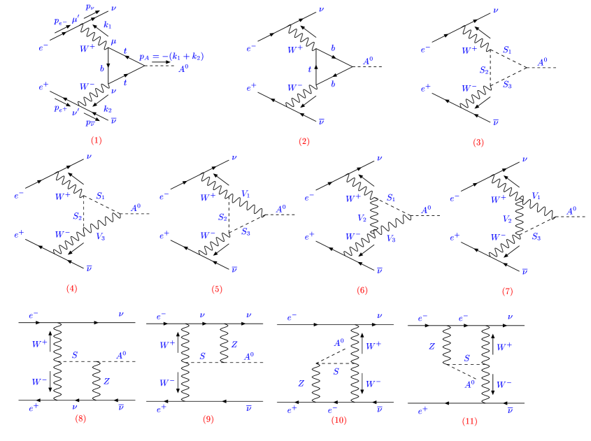
Figure 1: Feynman diagrams for 2HDM contributions to $e^{+}e^{-}\to\nu\overline{\nu}A^{0}$ via $t$-channel processes. Here $S_{i}$ denotes Higgs and Goldstone bosons, $V_{i}$ denotes gauge bosons.

Diagrams (1)-(7) are the (finite) triangle loop corrections to the effective $W^{+}W^{-}A^{0}$ coupling, and diagrams (8)-(11) are the box diagrams. For on-shell $W$ bosons, the sum of diagrams (3)-(7) with Higgs bosons and vector bosons running in the loop must exactly cancel gunhabkao . But, in the present context, the $W$ bosons are virtual and the sum of these diagrams is non-zero. There is no $WWA^{0}$ counterterm contribution since the $WWA^{0}$ vertex is finite. In addition, there are no tadpole contributions since we have set the renormalized tadpoles to be zero. We shall refer to this collection of diagrams as the $t$-channel diagrams.

There are additional diagrams related to $s$-channel $\gamma,Z$ exchange; these are shown in Fig. 2.

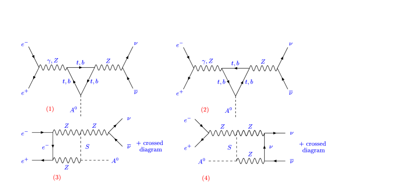
Figure 2: Feynman diagrams for 2HDM contributions to $e^{+}e^{-}\to\nu\overline{\nu}A^{0}$ via $s$-channel processes.

Diagrams (1) and (2) are the triangle loop contributions to the $\gamma ZA^{0}$ and $ZZA$ couplings (which are zero at tree-level), followed by $Z\to\nu\overline{\nu}$. Diagrams (3) and (4) are related box diagrams; photon exchanges do not appear in these diagrams because of the absence of $\gamma\nu\overline{\nu}$ and $\gamma ZS$ vertices. If the final exchanged $Z$ connected to $\nu\overline{\nu}$ is on-shell in diagrams (1)-(3), then the calculation is equivalent to $e^{+}e^{-}\to ZA^{0}$. This process has been calculated for the 2HDM and the full MSSM in Akeroyd:1999gu ; eeZAMSSM and the production cross section found to be small. The $Z$ resonant contribution to the $\nu\overline{\nu}A^{0}$ final state can be separated experimentally by detecting the $A^{0}$ in a visible final state (e.g. $b\overline{b}$), reconstructing the mass of the $\nu\overline{\nu}$ recoiling opposite the $A^{0}$ and removing events in which the reconstructed mass is near $m_{Z}$. However, far off-shell intermediate $Z$ bosons can potentially give $s$-channel contributions that interfere with the $t$-channel contributions to the $\nu\overline{\nu}A^{0}$ final state, and must be included in our calculation.

One possible concern is that including the $Z$ decay width in the $Z$ propagators in the diagrams of Fig. 2 might spoil the gauge invariance of the calculation. We checked explicitly and found that this is not the case. In particular, the sum of diagrams (1) and (2) in Fig. 2 is gauge invariant on its own. Also, there is a cancellation between the gauge-dependent part in diagram (3) and the corresponding crossed diagram. A similar cancellation occurs between the gauge-dependent part of diagram (4) and its crossed counterpart. All these cancellations occur as a result of numerator algebra and are independent of the $Z$ width appearing in the $Z$ propagators.

Another check of the gauge independence of our fixed width scheme for the $Z$ boson is to compare the numerical results to those of the “factorization scheme”, which is guaranteed to be gauge independent. Following, e.g., the discussion in Ref. nnHrcs , the one-loop matrix element in the factorization scheme is given by

$$\mathcal{M}=\frac{\hat{s}-m_{Z}^{2}}{\hat{s}-m_{Z}^{2}+im_{Z}\Gamma_{Z}}\mathcal{M}_{\Gamma_{Z}=0}.$$ (15)

The factorization scheme sets the nonresonant diagram (4) of Fig. 2 to zero when $\hat{s}=M_{Z}^{2}$, which leads to an effect of $\mathcal{O}(\alpha\Gamma_{Z}/M_{Z})\sim\mathcal{O}(\alpha^{2})$; since this is a higher-order effect, it should be small. Our results in the fixed width scheme agree numerically with those of the factorization scheme to within the precision of our phase space integration.

Another set of diagrams involving $Z-A^{0}$ mixing is given in Fig. 3.

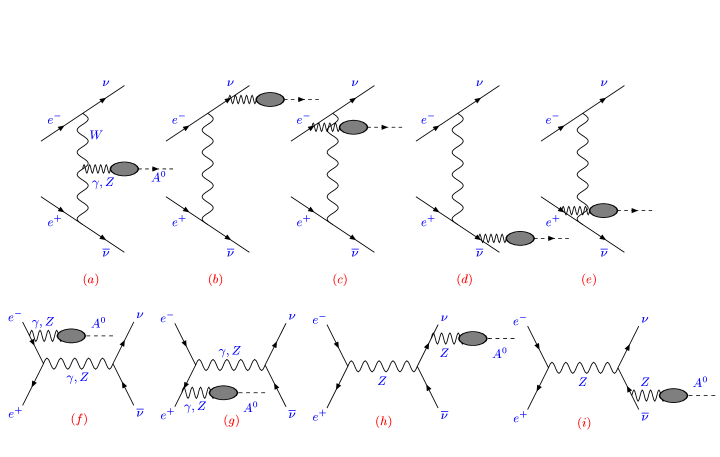
Figure 3: Feynman diagrams for the contribution to $e^{+}e^{-}\to\nu\overline{\nu}A^{0}$ through $Z$-$A^{0}$ and $\gamma$-$A^{0}$ mixing self-energies. The blob denotes the renormalized $Z$-$A^{0}$ and $\gamma$-$A^{0}$ mixing.

The contribution from diagram (a), in which the $W^{+}W^{-}$ couple to a virtual $Z^{*}$ which then mixes with the $A^{0}$ via (infinite) one-loop diagrams, is zero for on-shell $W$ bosons gunhabkao . With virtual $W$ bosons as in our case, diagram (a) is non-zero. However, it is not gauge invariant on its own. Additional diagrams (b)-(e) have to be taken into account. The sum of all these diagrams gives zero as a consequence of gauge invariance. This can be seen as follows. The one-particle-irreducible (1PI) two-point function for $Z-A^{0}$ mixing is defined as $-ip_{A}^{\mu}\Sigma_{Z-A^{0}}(p_{A}^{2})$, where $p_{A}^{\mu}$ is also the off-shell $Z$ momentum. Gauge invariance for the $Z$ tells us that after summing over all possible $Z$ attachments we must have $p_{A^{0}}^{\mu}{\cal A}_{\mu}=0$, where ${\cal A}_{\mu}$ is the full amplitude that would be dotted into the $Z$ propagator. In some renormalization schemes, one can also have $\gamma-A^{0}$ mixing, in which case a similar argument guarantees that after a complete sum over the diagrams (a), (c) and (e) with a virtual $\gamma^{*}$ one gets zero, just as in the $Z^{*}$ case. Of course, there are renormalization schemes (such as that chosen in Ref. cpr ) in which there is no $\gamma-A^{0}$ mixing and this issue does not arise. Similarly, the sum of $s$-channel diagrams (f)-(i) also gives zero.

The diagrams shown in Fig. 4 do not contribute to our calculation.

Figure 4: Contributions to $e^{+}e^{-}\to\nu\overline{\nu}A^{0}$ that we neglect. The blob denotes the renormalized $W^{\pm}$-$H^{\pm}$ mixing in diagrams (a) and (b) and the renormalized $(\gamma,Z)$-$(h^{0},H^{0})$ mixing in diagrams (c) and (d).

For diagrams (a) and (b), the one-loop $W^{+}\to H^{+}$ mixing graph must be proportional to $k_{W^{+}}^{\mu}=p_{\nu}^{\mu}-p_{e^{-}}^{\mu}$ (for example) , which gives zero when acting on the $V_{\mu}\overline{\nu}\gamma^{\mu}e$ vertex by the equation of motion. (Here we take the approximation that both electron and neutrino are massless.) Similarly, diagrams (c) and (d) also vanish.

Let us define $p_{e^{-}}$, $p_{e^{+}}$, $p_{\nu}$, $p_{\overline{\nu}}$, $k_{1}=p_{\nu}-p_{e^{-}}$ and $k_{2}=p_{\overline{\nu}}-p_{e^{+}}$ to be the momentum for the incoming electron, positron, outgoing neutrino, anti-neutrino, intermediate $W^{+}$ and $W^{-}$, respectively. The $t$-channel matrix element for $e^{+}e^{-}\to\nu\overline{\nu}A^{0}$ can be decomposed as follows (using $\xi=1$ Feynman-’t Hooft gauge):

$$\mathcal{M}_{t} = \frac{g^{2}}{2}{\overline{v}(p_{e^{+}},s_{e^{+}})\gamma_{\nu}P_{L}v(p_{\overline{\nu}},s_{\overline{\nu}})\over k_{1}^{2}-m_{W}^{2}}{\overline{u}(p_{\nu},s_{\nu})\gamma_{\mu}P_{L}u(p_{e^{-}},s_{e^{-}})\over k_{2}^{2}-m_{W}^{2}}$$ (16)

$$\times\left[F\epsilon^{\alpha\beta\mu\nu}k_{1\,\alpha}k_{2\,\beta}+Gg^{\mu\nu}+H_{1}p_{e^{-}}^{\nu}p_{e^{+}}^{\mu}+H_{2}p_{\nu}^{\nu}p_{\overline{\nu}}^{\mu}+H_{3}(-p_{e^{-}}^{\nu}p_{\overline{\nu}}^{\mu})+H_{4}(-p_{\nu}^{\nu}p_{e^{+}}^{\mu})\right],$$

where $P_{L}=(1-\gamma_{5})/2$. For the triangle loops [Fig. 1 diagrams (1)-(7)], only the combination $k_{1}^{\nu}k_{2}^{\mu}$ appears for the $H_{i}$ term. Therefore, the terms inside the square brackets in Eq. (16) can be simplified as

$$\left[F\epsilon^{\alpha\beta\mu\nu}k_{1\,\alpha}k_{2\,\beta}+Gg^{\mu\nu}+Hk_{1}^{\nu}k_{2}^{\mu}\right],$$ (17)

where $H=H_{1}=H_{2}=H_{3}=H_{4}$. Recall that the index $\mu$ ($\nu$) is associated with the $W^{+}$ ($W^{-}$) going into the $e^{-}$ ($e^{+}$) line. Analytical formulae for each Feynman diagram contribution to $F$, $G$, $H_{i}$ are summarized in Appendix B. In the on-shell limit where $k_{1}^{2}=k_{2}^{2}=m_{W}^{2}$, $G$ and $H$ are both zero gunhabkao , which can be seen explicitly in the analytical formulas.

The $s$-channel matrix element can be written as two non-interfering pieces: $\mathcal{M}_{s}=\mathcal{M}_{s}(e^{-}_{L}e^{+}_{R})+\mathcal{M}_{s}(e^{-}_{R}e^{+}_{L})$, where

$$\mathcal{M}_{s}(e^{-}_{L}e^{+}_{R})=\sum_{i\ {\rm even}}\mathcal{M}_{i}\mathcal{O}_{i},\qquad\mathcal{M}_{s}(e^{-}_{R}e^{+}_{L})=\sum_{i\ {\rm odd}}\mathcal{M}_{i}\mathcal{O}_{i}.$$ (18)

The definitions of the operators $\mathcal{O}_{i}$ and the contribution of Fig. 2 to $\mathcal{M}_{i}$ are given in Appendix C.

The spin averaged matrix element squared is:

$${1\over 4}{\sum}_{spins}|{\cal M}|^{2} = {1\over 4}{\sum}_{spins}|{\cal M}_{t}|^{2}+{3\over 4}{\sum}_{spins}|\mathcal{M}_{s}(e^{-}_{L}e^{+}_{R})|^{2}+{3\over 4}{\sum}_{spins}|\mathcal{M}_{s}(e^{-}_{R}e^{+}_{L})|^{2}$$ (19)

$$+ {1\over 4}{\sum}_{spins}{\cal M}_{t}\mathcal{M}_{s}(e^{-}_{L}e^{+}_{R})^{*}+{\rm h.c.},$$

which is used in the cross section calculations. The factor of 3 in the second and third terms represents the sum over the three neutrino flavors in the $s$-channel contribution. Notice that only the matrix element $\mathcal{M}_{s}(e^{-}_{L}e^{+}_{R})$ interferes with the $t$-channel diagrams, while the other $s$-channel matrix element does not. The explicit expression for the pieces in Eq. (19) is given in Appendix D.

Our numerical computations were performed using the LoopTools package Hahn:1998yk . We thus write the Appendices using the notation of LoopTools Hahn:1998yk for the one-loop integrals.

IV Numerical Results

IV.1 2HDM with tree-level MSSM mass and coupling relations

In this section, we give results for the $e^{+}e^{-}\to\nu\overline{\nu}A^{0}$ cross section as a function of $m_{A^{0}}$ and $\tan\beta$ assuming a type-II 2HDM with the tree-level MSSM constraints on the quartic couplings in the Higgs potential. As a result, the masses $m_{h^{0}}$, $m_{H^{0}}$ and $m_{H^{\pm}}$ and the mixing angle $\alpha$ of the CP-even sector are all fixed in terms of $m_{A^{0}}$ and $\tan\beta$ by the tree-level relations of the MSSM. The tree-level MSSM couplings lead to a theoretical upper bound on the mass of the lighter CP-even $h^{0}$ of $m_{h^{0}}\leq m_{Z}$ (which is increased to $\sim 135~{}{\rm GeV}$ by radiative corrections hmass ). In the decoupling region of large $m_{A^{0}}$ (typically $m_{A^{0}}\mathrel{\raise 1.29167pt\hbox{$>$\kern-7.5pt\lower 4.30554pt\hbox{$\sim$}}}2m_{Z}$ is large enough), the only light Higgs boson is the CP-even $h^{0}$, whose couplings to the SM particles approach their SM values. The other Higgs bosons $H^{0}$, $A^{0}$ and $H^{\pm}$ can be as heavy as a TeV. The heavy Higgs bosons are nearly degenerate in mass, with mass splittings of the order of $m_{Z}^{2}/m_{A^{0}}$.

Our choice of the tree-level MSSM Higgs sector can be thought of simply as a representative model choice within the 2HDM that gives decoupling and a SM-like $h^{0}$ as $m_{A^{0}}$ gets large. It will allow us to explain general features of the cross section and how they depend upon $m_{A^{0}}$ and $\tan\beta$. We will only examine results for $\tan\beta>1$ in this section. Our focus will be on situations in which $m_{A^{0}}\geq E_{cm}/2$, implying that pair production of the $A^{0}$ (e.g., $e^{+}e^{-}\to\nu\overline{\nu}A^{0}A^{0}$) will be kinematically forbidden, as will $e^{+}e^{-}\to A^{0}H^{0}$, since $m_{H^{0}}\simeq m_{A^{0}}$ for MSSM-like mass relations. The $e^{+}e^{-}\to h^{0}A^{0}$ process will also be strongly suppressed for $m_{A^{0}}\mathrel{\raise 1.29167pt\hbox{$>$\kern-7.5pt\lower 4.30554pt\hbox{$\sim$}}}2m_{Z}$. Thus, we are considering situations in which $A^{0}$ discovery might only be possible via the (one-loop) single $A^{0}$ production mechanisms that we consider.

The first feature of interest is that the $s$-channel and $t$-channel contributions to the cross section have different behavior as the collider center-of-mass energy increases, as shown in Fig. 5.

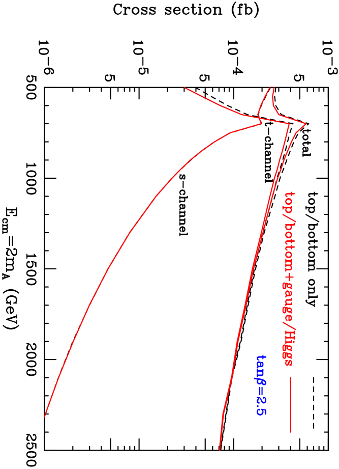
Figure 5: Behavior of the $t$- and $s$-channel contributions to $e^{+}e^{-}\to\nu\overline{\nu}A^{0}$ with $E_{cm}$. Here $\tan\beta=2.5$ and $m_{A^{0}}=E_{cm}/2$. The line labeled “total” shows the sum of the $t$- and $s$-channel contributions including their interference. The $s$-channel results including gauge/Higgs contributions are indistinguishable from the $s$-channel results with only top/bottom loops.

In particular, for $m_{A^{0}}=E_{cm}/2$, the $s$-channel contribution dominates for $E_{cm}\mathrel{\raise 1.29167pt\hbox{$<$\kern-7.5pt\lower 4.30554pt\hbox{$\sim$}}}650$ GeV, while the $t$-channel contribution dominates for $E_{cm}\mathrel{\raise 1.29167pt\hbox{$>$\kern-7.5pt\lower 4.30554pt\hbox{$\sim$}}}700$ GeV. To some extent the $s$- and $t$-channel contributions can be separated experimentally. For example, the $s$-channel contributions can be isolated by looking at $ZA^{0}$ final states in which the $Z$ decays to an observable final state, such as $q\overline{q}$ or $\ell^{+}\ell^{-}$. The $t$-channel contributions can be isolated to a large extent by looking at the $A^{0}$ in a visible final state decay mode (for example, $b\overline{b}$ or $\tau^{+}\tau^{-}$), reconstructing the mass recoiling against the $A^{0}$, and demanding that this recoil mass not be close to $m_{Z}$. In this latter case, this selection procedure would reduce somewhat the $t$-channel cross sections presented (which are integrated over all recoil masses).

Perhaps most importantly, we find that the cross sections are quite small, generally below 0.001 fb. This holds even for rather low values of $m_{A^{0}}$. The cross section as a function of $m_{A^{0}}$ is shown in Fig. 6.

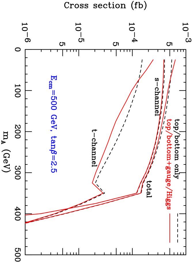
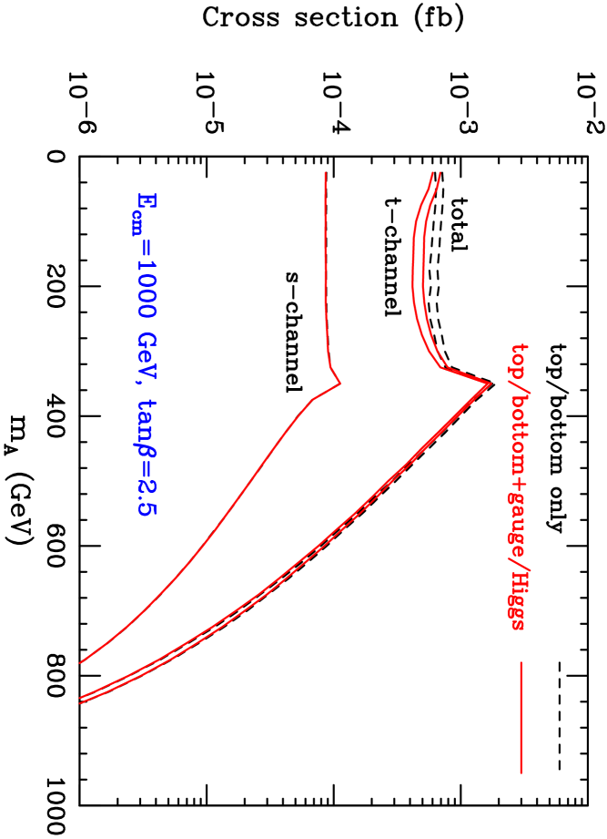
Figure 6: Cross section for $e^{+}e^{-}\to\nu\overline{\nu}A^{0}$ as a function of $m_{A^{0}}$, for $\tan\beta=2.5$ and $E_{cm}=500$ GeV (left) and 1000 GeV (right). The line labeled “total” shows the sum of the $t$- and $s$-channel contributions including their interference. As in the previous figure, the $s$-channel top/bottom only and top/bottom+gauge/Higgs lines are essentially identical. In the $E_{\rm cm}=1000~{}{\rm GeV}$ plot, we note that the “$t$-channel” lines (whether top/bottom only or top/bottom+gauge/Higgs) are always below the “total” lines in the $m_{A^{0}}\sim 200~{}{\rm GeV}$ region. Thus, for instance, the upper dashed line is the total “top/bottom only” result while the lower dashed line is the $t$-channel “top/bottom only” result.

This figure shows the expected peak in $\sigma(\nu\overline{\nu}A^{0})$ at $m_{A^{0}}\sim 2m_{t}$ from the top quarks in the loop going on shell, followed by a rapid fall as one approaches the kinematic limit at $m_{A^{0}}=\sqrt{s}$. Notice that for $E_{cm}=500$ GeV, the $s$-channel contribution dominates, while for $E_{cm}=1000$ GeV, the $t$-channel contribution dominates, as expected from Fig. 5. Similar results were presented in Ref. Arhrib:2002ti . While we include all three flavors of neutrinos in the final state since they are experimentally indistinguishable, Ref. Arhrib:2002ti included only $\nu_{e}\bar{\nu}_{e}$ in the final state, leading to an $s$-channel cross section smaller by a factor of 3 than our result. Taking this into account, our results are in rough agreement with those of Ref. Arhrib:2002ti . For example, for the point $E_{cm}=500$ GeV, $m_{A}=100$ GeV, $\tan\beta=2.5$, and one neutrino flavor, our result is about a factor of two larger than that shown in Fig. 4 of Ref. Arhrib:2002ti . Part of the discrepancy, a factor of $(137/128)^{4}=1.3$, is explained by the use of $\alpha=1/137$ in Ref. Arhrib:2002ti versus our use of $\alpha=1/128$.

The dependence of the cross section on $\tan\beta$ is shown in Fig. 7.

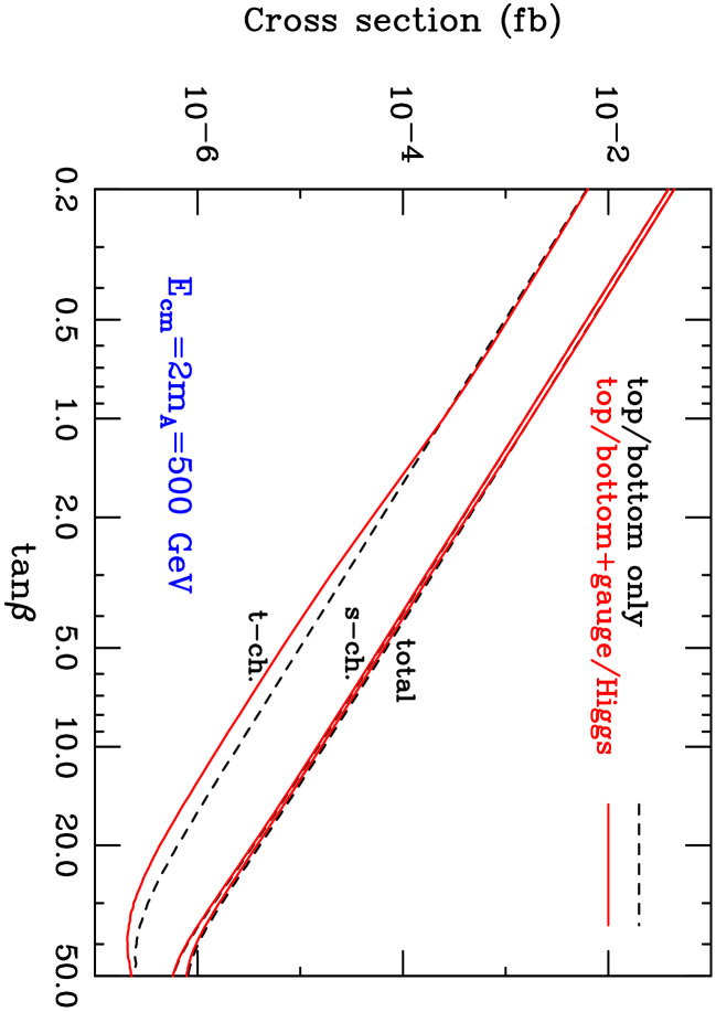
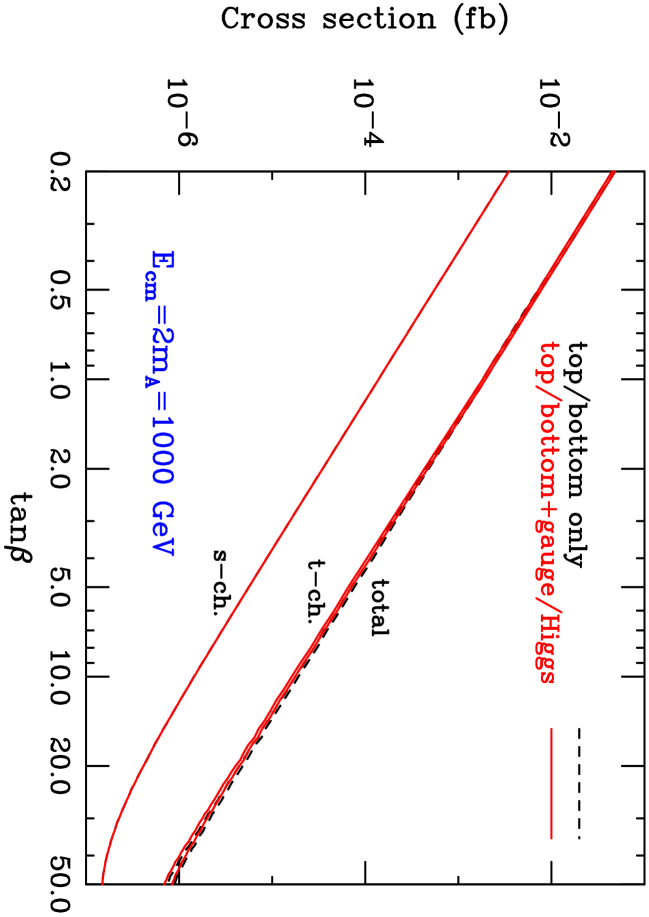
Figure 7: $\tan\beta$ dependence of the cross section for $e^{+}e^{-}\to\nu\overline{\nu}A^{0}$, for $E_{cm}=2m_{A^{0}}=500$ GeV (left) and 1000 GeV (right). As in the previous two figures, the $s$-channel curves with and without the gauge/Higgs contributions are indistinguishable. In the $E_{\rm cm}=500~{}{\rm GeV}$ ($E_{\rm cm}=1000~{}{\rm GeV}$) case, the “total” curves are slightly higher than the “$s$-ch.” (“$t$-ch.”) curves for both “top/bottom only” and for “top/bottom+gauge/Higgs”. The “top/bottom only” curves are slightly above the “top/bottom+gauge/Higgs” curves in both the “$s$-ch.” (“$t$-ch.”) and “total” cases. In this figure, we have used the shorthand “ch.” for “channel”.

This plot clearly shows that for the MSSM-like parameter relations, detection of the $\nu\overline{\nu}A^{0}$ final state will only be possible if $\tan\beta\mathrel{\raise 1.29167pt\hbox{$<$\kern-7.5pt\lower 4.30554pt\hbox{$\sim$}}}1$. The cross section falls like a power law with increasing $\tan\beta$. This is due to the fermion triangle diagrams with a top quark coupling to $A^{0}$ (diagram (1) in Fig. 1 and the $t$-loop case for diagrams (1) and (2) in Fig. 2), which dominate at low $\tan\beta$ and give a cross section proportional to $y_{t}^{2}\sim(\tan\beta)^{-2}$. At large values of $\tan\beta\mathrel{\raise 1.29167pt\hbox{$>$\kern-7.5pt\lower 4.30554pt\hbox{$\sim$}}}30$, the fermion triangle diagrams with a bottom quark coupling to $A^{0}$ (diagram (2) in Fig. 1 and the $b$-loop case for diagrams (1) and (2) in Fig. 2) begin to contribute significantly and affect the dependence on $\tan\beta$, since these diagrams give a cross section proportional to $y_{b}^{2}\sim(\tan\beta)^{2}$.

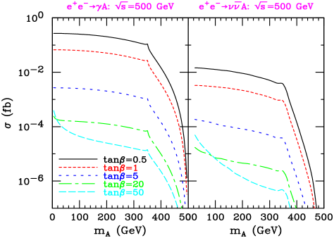
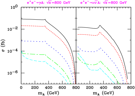
Figure 8: The $e^{+}e^{-}\to\gamma A^{0}$ and $\nu\overline{\nu}A^{0}$ cross sections as a function of $m_{A^{0}}$ for $\sqrt{s}=E_{\rm cm}=500~{}{\rm GeV}$ and $800~{}{\rm GeV}$, for $\tan\beta=0.5,1,5,20,50$. We employ the tree-level MSSM parameterization. The $e^{+}e^{-}\to\nu\overline{\nu}A^{0}$ cross section includes all contributions.

Another perspective on these results, and a comparison to the $e^{+}e^{-}\to\gamma A^{0}$ process Djouadi:1996ws ; Akeroyd:1999gu is presented in Fig. 8. For the tree-level MSSM type of 2HDM parameter choices, the $e^{+}e^{-}\to\gamma A^{0}$ process would probably lead to earlier discovery of the $A^{0}$ than would the $e^{+}e^{-}\to\nu\overline{\nu}A^{0}$ assuming both have small background. However, as described in the next section, the $e^{+}e^{-}\to\nu\overline{\nu}A^{0}$ can be enhanced for non-decoupling 2HDM parameter choices that lead to large Higgs self-couplings, whereas the $e^{+}e^{-}\to\gamma A^{0}$ cross section is not sensitive to Higgs self-couplings and would not be enhanced in such a parameter regime. Note also that the advantage of the $e^{+}e^{-}\to\gamma A^{0}$ process over the $e^{+}e^{-}\to\nu\overline{\nu}A^{0}$ process decreases slowly with increasing $E_{\rm cm}$, as seen from the figure by comparing the results for $E_{\rm cm}=500~{}{\rm GeV}$ to those for $E_{\rm cm}=800~{}{\rm GeV}$.

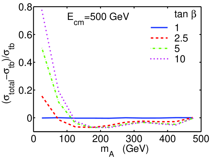
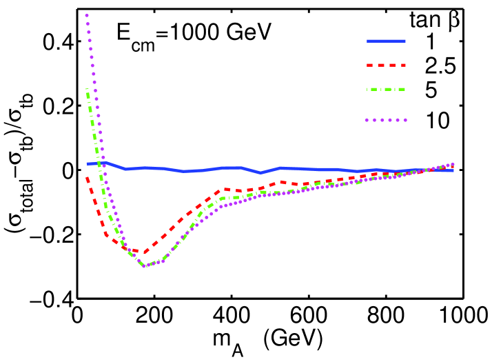
Figure 9: Contribution of the gauge and Higgs boson loops relative to the top and bottom quark loops, as a function of $m_{A^{0}}$. Plotted is the gauge and Higgs contribution normalized to the top and bottom quark contribution, $(\sigma_{total}-\sigma_{tb})/\sigma_{tb}$.

The relative size of the gauge and Higgs boson contributions compared to the top and bottom quark contributions is illustrated in Fig. 9. For $\tan\beta=1$, the gauge and Higgs boson loops vanish. For larger values of $\tan\beta$, the contribution of the gauge and Higgs boson loops relative to that of the top and bottom quark loops typically increases with increasing $\tan\beta$. At $E_{cm}=500$ GeV, the gauge and Higgs boson contributions can be quite significant at low $m_{A^{0}}\mathrel{\raise 1.29167pt\hbox{$<$\kern-7.5pt\lower 4.30554pt\hbox{$\sim$}}}100$ GeV, especially for larger values of $\tan\beta$. However, in the MSSM, $m_{A^{0}}\mathrel{\raise 1.29167pt\hbox{$<$\kern-7.5pt\lower 4.30554pt\hbox{$\sim$}}}92$ GeV is excluded by the LEP II data lepa ; lep2 . For larger values of $m_{A^{0}}$, the gauge and Higgs loops interfere destructively with the dominant top and bottom quark loops, resulting in a reduction of the cross section by less than 10%. At $E_{cm}=1000$ GeV, in contrast, the destructive interference of the gauge and Higgs boson loops with the top and bottom quark loops is much more significant for $m_{A^{0}}$ below the top quark pair production threshold of 350 GeV, suppressing the cross section by as much as 30% for $m_{A^{0}}\sim 200$ GeV. For $m_{A^{0}}\mathrel{\raise 1.29167pt\hbox{$>$\kern-7.5pt\lower 4.30554pt\hbox{$\sim$}}}350$ GeV, the gauge and Higgs boson loops reduce the cross section by less than 10%. The change in the relative size of the gauge and Higgs boson loops at different center-of-mass energies can be understood as follows. At $E_{cm}=500$ GeV, the cross section is dominated by the $s$-channel diagrams. The gauge and Higgs boson contributions to the $s$-channel matrix element come only from box diagrams [diagrams (3) and (4) in Fig. 2]. At $E_{cm}=1000$ GeV, the cross section is dominated by the $t$-channel diagrams. The gauge and Higgs boson contributions to the $t$-channel matrix element come from both triangle diagrams and box diagrams [diagrams (3)-(7) and (8)-(11), respectively, in Fig. 1]. The gauge and Higgs boson triangle diagrams in general give larger contributions to the cross section than the box diagrams, leading to larger gauge and Higgs boson contributions to the $t$-channel process than to the $s$-channel process. This behavior can also be seen in Fig. 6.

IV.2 General 2HDM

There is, of course, much more freedom in the general 2HDM than we have allowed for in the previous section First, there is the possibility of allowing for type-I fermionic couplings as opposed to the type-II fermionic couplings employed so far. As shown in Eq. (13), the type-I $t\overline{t}$ coupling is the same as the type-II coupling. This implies that the dominant $t$ loop contribution to the $\nu\overline{\nu}A^{0}$ cross section will be unchanged. The type-I $b\overline{b}$ coupling is proportional to $\cot\beta$ as opposed to $\tan\beta$ for type-II coupling; this means that the $b$-loop contribution to the $\nu\overline{\nu}A^{0}$ cross section is never important for type-I couplings. Numerically, this implies that the leveling off of $\sigma(\nu\overline{\nu}A^{0})$ at $\tan\beta\mathrel{\raise 1.29167pt\hbox{$>$\kern-7.5pt\lower 4.30554pt\hbox{$\sim$}}}40$ in Fig. 7 (and eventual rise at still larger $\tan\beta$) would not take place for type-I couplings. There is also the possibility of so-called type-III fermion couplings in which the two Higgs doublets both couple to up and down type quarks. In general, such couplings yield flavor changing neutral currents that are too large compared to existing experimental constraints. In addition, the numerical modifications to the type-II predictions already given would not be large. Thus, we do not consider type-I or type-III couplings further.

A second variation in the general 2HDM context is to allow for CP-violating couplings. As explained in the introduction, we have chosen not to explore this possibility here as it makes the $A^{0}$ less unique and because considerable cancellations between CP-violating contributions deriving from the Higgs sector are required for consistency between the computed EDMs and $(g_{\mu}-2)$ and experimental data. If the Higgs sector is CP-violating, all the neutral Higgs bosons mix and will all have some level of $VV$ coupling. In most scenarios, all three of the neutral Higgs bosons $h_{i}$ ($i=1,2,3$) would be easily detected in $Zh_{i}$ production and the tree-level contributions to the $\nu\overline{\nu}h_{i}$ ($i=1,2,3$) cross sections would all be considerably larger than the one-loop contributions Akeroyd:2001kt .

The most interesting issue in the general CP-conserving 2HDM context is the extent to which the Higgs self-couplings could deviate from those in our previous MSSM-like analysis, so that $\sigma(\nu\overline{\nu}A^{0})$ might be substantially increased or decreased by the Higgs boson loops compared to the value obtained from the $t$ and $b$ loops. In Fig. 9 we found that with MSSM-like couplings, the gauge and Higgs boson loops could change the cross section by as much as 70% compared to the $t$ and $b$ quark contributions for low values of $m_{A^{0}}$, or by up to 30% for $m_{A^{0}}\mathrel{\raise 1.29167pt\hbox{$>$\kern-7.5pt\lower 4.30554pt\hbox{$\sim$}}}m_{Z}$. Here, we explore the effect of removing the MSSM constraint on the Higgs boson self-couplings $\lambda_{i}$, while still requiring that they remain perturbative. (Following Gunion:2002zf , we define perturbativity by the requirement $\lambda_{i}/(4\pi)\mathrel{\raise 1.29167pt\hbox{$<$\kern-7.5pt\lower 4.30554pt\hbox{$\sim$}}}{\cal O}(1)$.) Another constraint on the 2HDM parameters derives from precision electroweak data, as conveniently summarized by the $S$ and $T$ parameters. We will explore the extent to which the $\nu\overline{\nu}A^{0}$ cross section can be enhanced via the triangle graphs involving Higgs self-couplings while remaining consistent with the perturbativity and $S,T$ constraints. In the preceding section, we considered parameter choices that correspond to rapid decoupling as $m_{A^{0}}$ increases beyond $\mathcal{O}(m_{Z})$. The Higgs self-coupling effects are likely to be most significant in those regions of parameter space that are far from the decoupling limit.

The triangle diagrams involving one or more internal gauge bosons, Fig. 1 diagrams (4)-(7), are controlled by $VSS$ and $VVS$ couplings which are determined by gauge invariance. The size of these couplings is limited, as shown in Tables 2 and 3. Any significant enhancement must come from the purely Higgs loop graph of Fig. 1 diagram (3), which is controlled by the Higgs self-couplings given in Table 1. For the diagrams in Fig. 1 diagram (3) involving one or more Goldstone bosons, the couplings are determined by gauge invariance purely in terms of the Higgs masses, the angle combination $\beta-\alpha$ and the weak mixing angle $\theta_{W}$ (see Table 1). For the diagrams with $h^{0}H^{+}A^{0}$ or $H^{0}H^{+}A^{0}$ running in the loop, on the other hand, the couplings $g_{A^{0}A^{0}h^{0}}$ and $g_{A^{0}A^{0}H^{0}}$ are determined by the invariant combinations of the $\lambda_{i}$, denoted by $\lambda_{T}$ and $\lambda_{U}$ in Ref. Gunion:2002zf , given in Eqs. (41) and (42). These couplings are free to vary in the general 2HDM once the MSSM constraints are removed. We will employ the ratios $\lambda_{U}/(4\pi)$ and $\lambda_{T}/(4\pi)$ to quantify the perturbativity of the self-couplings. Numbers much larger than 1 for these ratios imply that the self-couplings are becoming non-perturbative and that higher order corrections to the results we obtain could be large.

Our procedure will be to choose values for the Higgs masses $m_{A^{0}}$, $m_{h^{0}}$ and $m_{H^{0}}$ and for $\tan\beta$, and then scan over $\alpha$ and $m_{H^{\pm}}$ selecting points that are consistent with the experimental $S,T$ values at the 95% CL. As in Ref. Chankowski:2000an (see also Gunion:2002zf ), for simplicity we will restrict $\lambda_{4}$ relative to $\lambda_{5}$ by requiring $\lambda_{4}=-\lambda_{5}$, implying $\lambda_{5}v^{2}=(m_{H^{\pm}}^{2}-m_{A^{0}}^{2})$. This choice makes it relatively easy to find values for the other parameters that give good agreement with precision electroweak $S,T$ data. Indeed, as discussed in Ref. Chankowski:2000an , even if we choose large values for $m_{h^{0}}$ and $m_{H^{0}}$ (in particular, beyond the kinematic reach of the linear collider), it is nonetheless possible to choose $\alpha$ and $m_{H^{\pm}}$ in such a way that the $S,T$ values are within the 95% CL ellipse. The key is to have $m_{H^{\pm}}>m_{h^{0}},m_{H^{0}}$ by a small amount (typically 10 to 30 GeV) in such a way that the large negative $\Delta T$ generated by the heavy neutral scalar(s) with substantial $VV$ coupling is compensated by an even larger positive $\Delta T$ contribution coming from the $m_{H^{\pm}}-m_{h^{0}}$ and/or $m_{H^{\pm}}-m_{H^{0}}$ mass difference. As one varies $\alpha$ at fixed $\tan\beta$, it is generally possible to adjust the value of $m_{H^{\pm}}$ in such a way as to remain within the (upper right hand segment of the) 95% CL $S$-$T$ ellipse.

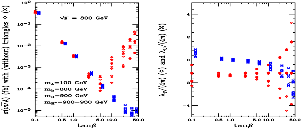
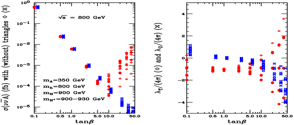
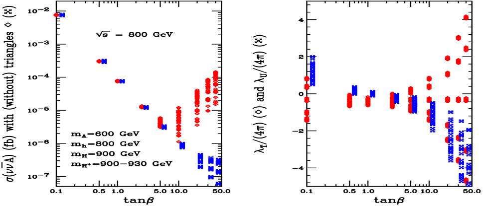
Figure 10: Left-hand graphs: $\sigma(\nu\overline{\nu}A^{0})$ as a function of $\tan\beta$ for $E_{cm}=800$ GeV, with (points slightly to the left) and without (points slightly to the right) Higgs-self-coupling triangle diagrams. Right-hand graphs: corresponding values of $\lambda_{T,U}/(4\pi)$. (We do not attempt to display point-to-point matching between the left-hand and right-hand plots.) The three plots are for $m_{A^{0}}=100,350,600~{}{\rm GeV}$, $m_{h^{0}}=800~{}{\rm GeV}$, $m_{H^{0}}=900~{}{\rm GeV}$ and $m_{H^{\pm}}\in[900,930]~{}{\rm GeV}$. The plotted points have $m_{H^{\pm}}$ and $\alpha$ chosen so that $S,T$ lie within the 95% CL precision electroweak data ellipse.

We show the results of this procedure in Fig. 10. We compute $\sigma(\nu\overline{\nu}A^{0})$ for $m_{A^{0}}=100$, $350$, and $600~{}{\rm GeV}$ as a function of $\tan\beta$, assuming a collider energy of $\sqrt{s}=800~{}{\rm GeV}$. We take $m_{h^{0}}=800~{}{\rm GeV}$ and $m_{H^{0}}=900~{}{\rm GeV}$ and scan over $0\leq\alpha\leq\pi$ in 10 steps and over $m_{H^{\pm}}$ in steps of $10~{}{\rm GeV}$ beginning with $m_{H^{0}}$ as the lowest value. In particular, all the Higgs masses other than $m_{A^{0}}$ are chosen such that none of the other Higgs bosons can be produced for the assumed collider energy. We plot only those points for which the $S,T$ values are within the 95% CL precision electroweak ellipse. In the left-hand plots of Fig. 10 we give $\sigma(\nu\overline{\nu}A^{0})$ with and without including the Feynman diagrams containing Higgs self-couplings. In the right-hand plots of Fig. 10, we plot the corresponding values of $\lambda_{T}/(4\pi)$ and $\lambda_{U}/(4\pi)$ (without attempting a point-by-point identification). We observe that the Higgs self-coupling diagrams can have a very large effect on the cross section at large $\tan\beta$ if one is willing to accept values of $\lambda_{T,U}/(4\pi)$ of order 2 to 3. At large $\tan\beta$, the cross section is very substantially enhanced by the self-coupling graphs and might be visible with $L=1000~{}{\rm fb}^{-1}$ of integrated luminosity. Certainly, detection of this cross section would be an extremely interesting and important probe of the Higgs self-couplings, especially given that all Higgs bosons other than the $A^{0}$ are too heavy to observe directly at the linear collider in the situations considered.

In short, the lesson of this section is that if nature chooses the Higgs sector parameters to be far from the decoupling regime, it could happen that only the $A^{0}$ will be within the kinematic reach of the linear collider and that the $\nu\overline{\nu}A^{0}$ cross section might be observable. If in the future the LHC finds a fairly heavy CP-even Higgs boson, then, within the 2HDM (or similar) context, the type of situation considered here will be required for consistency with current precision electroweak constraints and one should urgently search for the $A^{0}$ in single production modes.

IV.3 Special situations in the MSSM

In order to obtain a large cross section for $\nu\overline{\nu}A^{0}$ production in the MSSM when $\tan\beta>1$, the $t\overline{t}$ or $b\overline{b}$ coupling of the $A^{0}$ must be enhanced very substantially. This is within the realm of possibility. In particular, at large $\tan\beta$ it is possible to have important one loop modifications to the $A^{0}b\overline{b}$ coupling due to radiative corrections involving a gluino and a bottom squark. We briefly review this aspect of the MSSM and then show the resulting enhancement for favorable parameter choices.

Since supersymmetry is broken, the bottom quark will have, in addition to its usual tree-level coupling to the Higgs field $\Phi_{1}^{0}$, a small one-loop-induced coupling to $\Phi_{2}^{0}$ that couples to up quarks at tree-level:

$$-\mathcal{L}_{\rm Yukawa}\simeq h_{b}\Phi_{1}^{0}b\overline{b}+(\Delta h_{b})\Phi_{2}^{0}b\overline{b}\,.$$ (20)

When the Higgs doublets acquire their vacuum expectation values, the bottom quark mass receives an extra contribution equal to $(\Delta h_{b})v_{2}$. Although $\Delta h_{b}$ is one-loop suppressed relative to $h_{b}$, for sufficiently large values of $\tan\beta$ ($v_{2}\gg v_{1}$) the contribution to the bottom quark mass of both terms in Eq. (20) may be comparable in size. This induces a large modification in the tree–level relation,

$$m_{b}={h_{b}v_{1}\over\sqrt{2}}(1+\Delta_{b})\,,\qquad$$ (21)

where $\Delta_{b}\equiv(\Delta h_{b})\tan\beta/h_{b}$. The function $\Delta_{b}$ contains two main contributions: one from a bottom squark–gluino loop (which depends on the two bottom squark masses $m_{\tilde{b}_{1}}$ and $m_{\tilde{b}_{2}}$ and the gluino mass $m_{\tilde{g}}$) and another one from a top squark–higgsino loop (which depends on the two top squark masses $m_{\tilde{t}_{1}}$ and $m_{\tilde{t}_{2}}$ and the higgsino mass parameter $\mu$). The explicit form of $\Delta_{b}$ at one-loop in the limit of $M_{S}\gg m_{b}$ is given by deltamb0 ; deltamb1 ; deltamb2 :

$$\Delta_{b}\simeq{2\alpha_{s}\over 3\pi}m_{\tilde{g}}\mu\tan\beta~{}I(m_{\tilde{b}_{1}},m_{\tilde{b}_{2}},m_{\tilde{g}})+{Y_{t}\over 4\pi}A_{t}\mu\tan\beta~{}I(m_{\tilde{t}_{1}},m_{\tilde{t}_{2}},\mu),$$ (22)

where $\alpha_{s}=g_{s}^{2}/4\pi$, $Y_{t}\equiv h_{t}^{2}/4\pi$, and contributions proportional to the electroweak gauge couplings have been neglected. The function $I$ is manifestly positive. Since the Higgs coupling proportional to $\Delta h_{b}$ is a manifestation of the broken supersymmetry in the low energy theory, $\Delta_{b}$ does not decouple in the limit of large supersymmetry breaking masses. Indeed, if all supersymmetry breaking mass parameters (and $\mu$) are scaled by a common factor, the correction $\Delta_{b}$ remains constant. For our purposes, the important implication is the modified form of the $b\overline{b}A^{0}$ coupling $y_{b}$ [compare Eq. (14)]:

$$y_{b}=\frac{m_{b}}{v}\frac{\tan\beta}{1+\Delta_{b}},$$ (23)

where $\Delta_{b}\propto\tan\beta$ [see Eq. (22)]. For appropriate parameter choices with $\mu<0$ (assuming the standard convention of $m_{\tilde{g}}>0$), $\Delta_{b}\sim-1$ will occur at some value of moderate to large $\tan\beta$. At and near this point, the triangle diagrams in our calculation involving the $b\overline{b}A^{0}$ coupling [diagram (2) of Fig. 1 and the $b$-loop cases of diagrams (1) and (2) of Fig. 2] will be greatly enhanced leading to a very large cross section. We illustrate this for the specific choices of $m_{A^{0}}=300~{}{\rm GeV}$, $\sqrt{s}=800~{}{\rm GeV}$, $\mu=-2~{}{\rm TeV}$, $m_{\widetilde{b}_{R}}=525~{}{\rm GeV}$, $m_{\widetilde{g}}=M_{2}=m_{\widetilde{\ell}_{L,R}}=m_{\widetilde{q}_{L,R}}=m_{\widetilde{b}_{L}}=m_{\widetilde{t}_{L,R}}=1~{}{\rm TeV}$, and $A_{t}=A_{b}=A_{\tau}=\mu/\tan\beta+\sqrt{6}m_{\widetilde{t}_{L}}$ (corresponding to maximal-mixing in the stop sector). Since $A_{t}\neq 0$ in general, both the gluino–bottom squark and higgsino–top squark loops contribute to $\Delta_{b}$. Note that we have chosen sufficiently large masses for the SUSY particles that the one-loop contributions to $e^{+}e^{-}\to\nu\overline{\nu}A^{0}$ involving them will be very suppressed. Keeping only the $WW$ fusion $t$ and $b$ loop diagrams [diagrams (1)-(2) of Fig. 1] for simplicity, we plot $\sigma(\nu\overline{\nu}A^{0})$ as a function of $\tan\beta$ for these parameter choices in Fig. 11, and compare to the result that would be obtained without including $\Delta_{b}$.

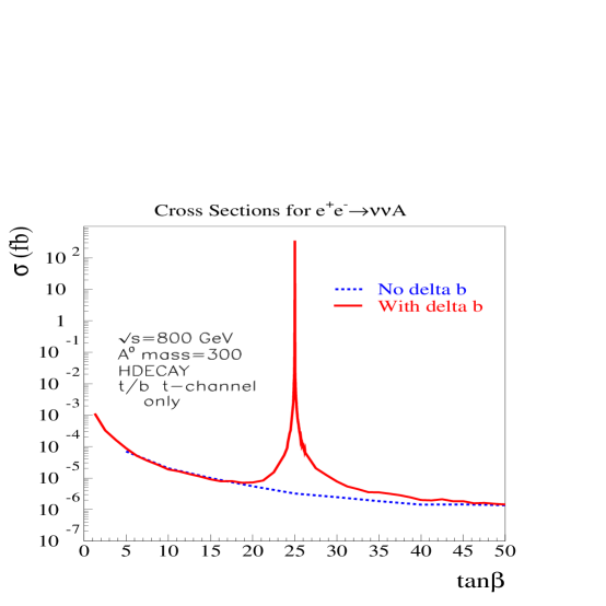
Figure 11: Dependence of $\sigma(\nu\overline{\nu}A^{0})$ on $\tan\beta$ for $m_{A^{0}}=300~{}{\rm GeV}$ and $\sqrt{s}=800~{}{\rm GeV}$, using HDECAY and MSSM parameters as specified in the text. Results are shown keeping only the (dominant) $t$-channel (i.e., $WW$ fusion) $t$ and $b$ fermion-loop graphs.

A close-up of the $\tan\beta$ region in which $\Delta_{b}\sim-1$ is shown in Fig. 12.

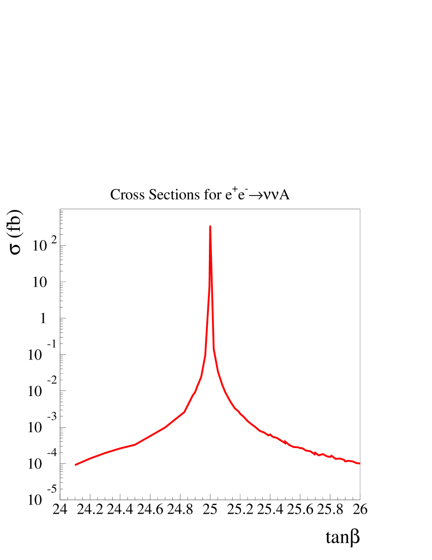
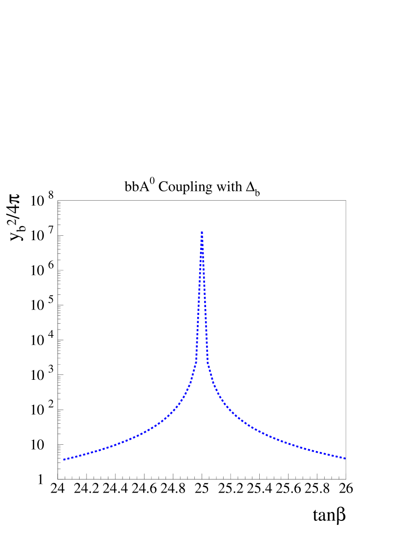
Figure 12: (Left) Dependence of $\sigma(\nu\overline{\nu}A^{0})$ on $\tan\beta$ as in Fig. 11, for $24\leq\tan\beta\leq 26$. (Right) The corresponding value of $y_{b}^{2}/(4\pi)$.

The plots show that for $\tan\beta$ within a few per mil of the point where $\Delta_{b}\sim-1$, the cross section can approach the femtobarn level. However, this corresponds to an extremely nonperturbative $b\overline{b}A^{0}$ coupling $y_{b}^{2}/(4\pi)\sim 10^{5}$. Requiring perturbativity, $y_{b}^{2}/(4\pi)\mathrel{\raise 1.29167pt\hbox{$<$\kern-7.5pt\lower 4.30554pt\hbox{$\sim$}}}\mathcal{O}(1)$, yields a cross section of order $10^{-4}$ fb, an enhancement of 1–2 orders of magnitude compared to the cross section without the $\Delta_{b}$ effects.

While it would be rather serendipitous for the MSSM parameters to be within the rather narrow range of $\tan\beta$ for which $\Delta_{b}$ is sufficiently near $-1$ to yield a significantly enhanced $e^{+}e^{-}\to\nu\overline{\nu}A^{0}$ cross section, one cannot simply rule the possibility out. Of course, if the one-loop enhancement is very large, higher loop corrections would need to be computed to more precisely evaluate the magnitude of the cross section enhancement.

V Conclusions

Detection of the CP-odd $A^{0}$ of a CP-conserving two-Higgs-doublet model via tree-level production mechanisms might not be possible due to: (a) the absence of $VVA^{0}$ ($V=W,Z$) tree-level couplings; (b) kinematic limitations such as $\sqrt{s_{e^{+}e^{-}}}<2m_{A^{0}},m_{A^{0}}+m_{H^{0}}$; and/or (c) the small size of the “Yukawa radiation” processes yielding $t\overline{t}A^{0}$ and $b\overline{b}A^{0}$ final states [as typical for intermediate $\tan\beta$ values in the “wedge” region of $(m_{A^{0}},\tan\beta)$ parameter space]. These difficulties become magnified in models with more than one CP-odd Higgs boson (the minimal such Higgs sector is that containing two-doublets plus one-singlet). Thus, it is generically important to compute single-$A^{0}$ production rates deriving from one-loop diagrams (i.e. not associated with $A^{0}$ radiation from a $b$ or $t$ quark) and ascertain the circumstances under which such processes might allow detection of the $A^{0}$. In this paper, we have computed the full (one-loop) cross section for $e^{+}e^{-}\to\nu\overline{\nu}A^{0}$ in the general CP-conserving 2HDM. Our results are presented in such a way that they can be easily extended to more complicated models containing a CP-odd Higgs boson. Complete formulae for the matrix elements are given in the Appendices.

We have presented numerical results for three cases in the context of the CP-conserving type-II 2HDM. The first case considered is that where the Higgs sector parameters are chosen using the tree-level MSSM Higgs sector constraints. For this choice, the 2HDM rapidly enters the “decoupling” regime once $m_{A^{0}}>m_{Z}$. For $\tan\beta>1$, the $e^{+}e^{-}\to\nu\overline{\nu}A^{0}$ cross section is typically rather small, especially for $m_{A^{0}}>2m_{t}$. However, for $\tan\beta<1$ we find that $e^{+}e^{-}\to\nu\overline{\nu}A^{0}$ production could provide a viable $A^{0}$ signal, thus covering this important part of the $(m_{A^{0}},\tan\beta)$ “wedge” parameter space region in the 2HDM where $A^{0}$ discovery using tree-level processes is not possible. In addition, if detected the $\nu\overline{\nu}A^{0}$ rate would provide a very sensitive constraint on $\tan\beta$.

For the decoupling 2HDM parameter choices considered above, the diagrams contributing to $\nu\overline{\nu}A^{0}$ production that involve Higgs self-couplings ($A^{0}A^{0}h^{0}$ and $A^{0}A^{0}H^{0}$) are typically smaller (often much smaller) in size than $t$- and $b$-loop diagrams involving $t\overline{t}A^{0}$ and $b\overline{b}A^{0}$ couplings. Thus, we have explored alternative 2HDM parameter choices for which one is far from the decoupling limit and the Higgs self-couplings are as large as they can be without violating perturbativity or precision electroweak constraints. We have found that substantial enhancement of the $e^{+}e^{-}\to\nu\overline{\nu}A^{0}$ cross section is possible when $\tan\beta>10$, possibly sufficient to make the process marginally observable. While $A^{0}$ discovery via the $\nu\overline{\nu}A^{0}$ final state would probably still be difficult, if the $A^{0}$ has been detected by other means and the approximate value of $\tan\beta$ is already known, the above results imply that $e^{+}e^{-}\to\nu\overline{\nu}A^{0}$ might provide an especially sensitive probe of the Higgs self-couplings of the 2HDM.

Finally, we considered the effect on the cross section of an enhancement of the $b\overline{b}A^{0}$ coupling caused by SUSY radiative corrections in the MSSM, parameterized by $\Delta_{b}$. While the $\Delta_{b}$ effects can enhance the cross section by 1–2 orders of magnitude while maintaining a perturbative $b\overline{b}A^{0}$ coupling, this enhancement typically occurs at moderate to large values of $\tan\beta$ where the cross section is already quite tiny, so that even with a $\Delta_{b}$ enhancement the cross section is not larger than about $10^{-4}$ fb.

For most parameter choices, the $e^{+}e^{-}\to\nu\overline{\nu}A^{0}$ cross section is smaller than other single $A^{0}$ production channels, most notably $e^{+}e^{-}\to\gamma A^{0}$. However, the two production modes are complementary in important respects. First, the $\nu\overline{\nu}A^{0}$ cross section could provide confirmation of a signal seen in the $\gamma A^{0}$ final state. Second, if $\tan\beta$ is not large, as might be known either because the two rates are fairly large or from other Higgs sector measurements, then $\Delta_{b}$ or Higgs self-coupling enhancements cannot be substantial and the determinations of $\tan\beta$ provided by the two processes can be fruitfully combined. Third, while the $\gamma A^{0}$ rate could also be enhanced by $\Delta_{b}$ effects it cannot be enhanced by large Higgs self-couplings (the needed $A^{0}H^{\pm}H^{\mp}$ and $ZH^{\pm}G^{\mp}$ vertices for the $H^{+}$-loop and $H^{+}$-$G^{+}$–loop, respectively, being absent in the 2HDM). Thus, an unexpectedly large cross section in the $e^{+}e^{-}\to\nu\overline{\nu}A^{0}$ channel would signal large Higgs self-couplings if a similar enhancement is not found in the $\gamma A^{0}$ final state. We note that this cross-check would be important even if no evidence for SUSY particles is found since a large $\Delta_{b}$ can arise for arbitrarily large SUSY particle masses.

An important extension of this work will be to include the contributions from one-loop diagrams that involve supersymmetric particles. For a light SUSY spectrum, very substantial enhancements could occur. This could be especially important in the following situation. Imagine that the LHC (or Tevatron) discovers fairly light SUSY particles and a SM-like $h^{0}$ but is unable to detect the heavier Higgs bosons $A^{0}$, $H^{0}$ and $H^{\pm}$. This situation arises at the LHC for moderate $\tan\beta$ values within the wedge beginning at $m_{A^{0}}\sim 200~{}{\rm GeV}$ and becoming rapidly wider in $\tan\beta$ as $m_{A^{0}}$ increases. If a linear $e^{+}e^{-}$ collider has too low a center-of-mass energy for $A^{0}H^{0}$ and $H^{+}H^{-}$ pair production, we must search for the $A^{0}$ (and the $H^{0}$ and $H^{\pm}$) in the single production modes. For a light enough SUSY spectrum these modes could be sufficiently enhanced to make $\gamma A^{0}$, $\nu\overline{\nu}A^{0}$ and similar processes observable, as found to be the case for $e^{+}e^{-}\to W^{\pm}H^{\mp}$ production Logan:2002jh .

Appendix A Notation and conventions

We follow the notation used on the LoopTools Hahn:1998yk web page (as of the date of this paper) for the one-loop integrals. To avoid any possible confusion, our explicit conventions are given below. The two-point integrals are:

$$\frac{i}{16\pi^{2}}\left\{B_{0},k^{\mu}B_{1}\right\}(k^{2},m_{1}^{2},m_{2}^{2})=\int\!\frac{d^{D}q}{(2\pi)^{D}}\frac{\{1,q^{\mu}\}}{(q^{2}-m_{1}^{2})((q+k)^{2}-m_{2}^{2})},$$ (24)

where $D$ is the number of dimensions.

Figure 13: Illustration of the LoopTools conventions employed for the triangle diagram case.

The three-point integrals are:

$$\frac{i}{16\pi^{2}}\left\{C_{0},C^{\mu},C^{\mu\nu}\right\}=\hskip 0.0pt\int\!\frac{d^{D}q}{(2\pi)^{D}}\frac{\{1,q^{\mu},q^{\mu}q^{\nu}\}}{(q^{2}-m_{1}^{2})((q+k_{1})^{2}-m_{2}^{2})((q+k_{2})^{2}-m_{3}^{2})},$$

where the denominator structure follows from the Feynman diagram of Fig. 13. The tensor integrals are decomposed in terms of scalar components as

$$C^{\mu} = k_{1}^{\mu}C_{1}+k_{2}^{\mu}C_{2}$$

$$C^{\mu\nu} = g^{\mu\nu}C_{00}+k_{1}^{\mu}k_{1}^{\nu}C_{11}+k_{2}^{\mu}k_{2}^{\nu}C_{22}+(k_{1}^{\mu}k_{2}^{\nu}+k_{2}^{\mu}k_{1}^{\nu})C_{12}.$$ (25)

The arguments of the scalar three-point integrals are specified in our convention as $(k_{1}^{2},(k_{2}-k_{1})^{2},k_{2}^{2},m_{1}^{2},m_{2}^{2},m_{3}^{2})$.

The four-point integrals are:

$$\frac{i}{16\pi^{2}}\left\{D_{0},D^{\mu},D^{\mu\nu}\right\}=\hskip 0.0pt\int\!\frac{d^{D}q}{(2\pi)^{D}}\frac{\{1,q^{\mu},q^{\mu}q^{\nu}\}}{(q^{2}-m_{1}^{2})((q+k_{1})^{2}-m_{2}^{2})((q+k_{2})^{2}-m_{3}^{2})((q+k_{3})^{2}-m_{4}^{2})},$$ (26)

where the tensor integrals are decomposed in terms of scalar components as

$$D^{\mu} = k_{1}^{\mu}D_{1}+k_{2}^{\mu}D_{2}+k_{3}^{\mu}D_{3}$$

$$D^{\mu\nu} = g^{\mu\nu}D_{00}+k_{1}^{\mu}k_{1}^{\nu}D_{11}+k_{2}^{\mu}k_{2}^{\nu}D_{22}+k_{3}^{\mu}k_{3}^{\nu}D_{33}$$ (27)

$$+(k_{1}^{\mu}k_{2}^{\nu}+k_{2}^{\mu}k_{1}^{\nu})D_{12}+(k_{1}^{\mu}k_{3}^{\nu}+k_{3}^{\mu}k_{1}^{\nu})D_{13}+(k_{2}^{\mu}k_{3}^{\nu}+k_{3}^{\mu}k_{2}^{\nu})D_{23}.$$

The arguments of the scalar four-point integrals are $(k_{1}^{2},(k_{2}-k_{1})^{2},(k_{3}-k_{2})^{2},k_{3}^{2},k_{2}^{2},(k_{1}-k_{3})^{2},m_{1}^{2},m_{2}^{2},m_{3}^{2},m_{4}^{2})$.

For the three-point functions $C_{i}$ and $C_{ij}$, it is useful to define the sums and differences of one-loop integrals as follows:

$$C^{S}_{i,ij}(k_{1}^{2},(k_{2}-k_{1})^{2},k_{2}^{2},m_{1}^{2},m_{2}^{2},m_{3}^{2}) = \frac{1}{2}\left[C_{i,ij}(k_{1}^{2},(k_{2}-k_{1})^{2},k_{2}^{2},m_{1}^{2},m_{2}^{2},m_{3}^{2})+C_{i,ij}((k_{2}-k_{1})^{2},k_{1}^{2},k_{2}^{2},m_{1}^{2},m_{2}^{2},m_{3}^{2})\right]$$

$$C^{D}_{i,ij}(k_{1}^{2},(k_{2}-k_{1})^{2},k_{2}^{2},m_{1}^{2},m_{2}^{2},m_{3}^{2}) = \frac{1}{2}\left[C_{i,ij}(k_{1}^{2},(k_{2}-k_{1})^{2},k_{2}^{2},m_{1}^{2},m_{2}^{2},m_{3}^{2})-C_{i,ij}((k_{2}-k_{1})^{2},k_{1}^{2},k_{2}^{2},m_{1}^{2},m_{2}^{2},m_{3}^{2})\right]$$

Appendix B 2HDM contributions to t-channel diagrams

We list here our results for the $t$-channel, i.e. $WW$-fusion, diagrams. In the expressions below, $k_{1}$ and $k_{2}$ denote the momenta of the $W^{+}$ and $W^{-}$, respectively, with directions such that $k_{1}=p_{\nu}-p_{e^{-}}$ and $k_{2}=p_{\overline{\nu}}-p_{e^{+}}$; see Fig. 1.1. (These $k_{1,2}$ should not be confused with those defining the LoopTools conventions in Appendix A.)

Fig. 1.1 ($ttb$ loop):

$$F_{t} = i{g^{3}m_{t}^{2}\cot\beta N_{c}\over 16m_{W}\pi^{2}}C_{2}^{S},$$ (29)

$$G_{t} = {g^{3}m_{t}^{2}\cot\beta N_{c}\over 32m_{W}\pi^{2}}\left[(k_{1}^{2}-k_{2}^{2})C_{2}^{S}-m_{A^{0}}^{2}C_{2}^{D}\right],$$ (30)

$$H_{t} = {g^{3}m_{t}^{2}\cot\beta N_{c}\over 16m_{W}\pi^{2}}C_{2}^{D}\,,$$ (31)

with the arguments for the integral functions as $C(k_{1}^{2},k_{2}^{2},m_{A^{0}}^{2},m_{t}^{2},m_{b}^{2},m_{t}^{2})$.

Fig. 1.2 ($bbt$ loop):

$$F_{b} = i{g^{3}m_{b}^{2}\tan\beta N_{c}\over 16m_{W}\pi^{2}}C_{2}^{S},$$ (32)

$$G_{b} = -{g^{3}m_{b}^{2}\tan\beta N_{c}\over 32m_{W}\pi^{2}}\left[(k_{1}^{2}-k_{2}^{2})C_{2}^{S}-m_{A^{0}}^{2}C_{2}^{D}\right],$$ (33)

$$H_{b} = -{g^{3}m_{b}^{2}\tan\beta N_{c}\over 16m_{W}\pi^{2}}C_{2}^{D}\,,$$ (34)

with the arguments for the integral functions as $C(k_{1}^{2},k_{2}^{2},m_{A^{0}}^{2},m_{b}^{2},m_{t}^{2},m_{b}^{2})$.

Fig. 1.3 ($SSS$ loop):

$$G_{SSS} = -\frac{ie^{3}}{2\pi^{2}}g_{AS_{1}S_{3}}g_{WS_{2}S_{1}}g_{WS_{3}S_{2}}C^{D}_{00},$$ (35)

$$H_{SSS} = -\frac{ie^{3}}{2\pi^{2}}g_{AS_{1}S_{3}}g_{WS_{2}S_{1}}g_{WS_{3}S_{2}}[C^{D}_{22}+C^{D}_{12}+C^{D}_{2}],$$ (36)

with the arguments for the integral functions as $C(k_{1}^{2},k_{2}^{2},m_{A^{0}}^{2},m_{1}^{2},m_{2}^{2},m_{3}^{2})$.

The combinations of scalar particles to be summed over and the respective couplings are given for the general type-II 2HDM in Table 1.

$S_{1}$	$S_{2}$	$S_{3}$	$g_{A^{0}S_{1}S_{3}}$	$g_{WS_{2}S_{1}}$	$g_{WS_{3}S_{2}}$
$h^{0}$	$H^{+}$	$A^{0}$	$g_{A^{0}A^{0}h^{0}}$	$-\cos(\beta-\alpha)/2s_{W}$	$-i/2s_{W}$
$H^{0}$	$H^{+}$	$A^{0}$	$g_{A^{0}A^{0}H^{0}}$	$\sin(\beta-\alpha)/2s_{W}$	$-i/2s_{W}$
$h^{0}$	$G^{+}$	$G^{0}$	$(m_{A^{0}}^{2}-m_{h^{0}}^{2})\cos(\beta-\alpha)/2m_{W}s_{W}$	$-\sin(\beta-\alpha)/2s_{W}$	$-i/2s_{W}$
$H^{0}$	$G^{+}$	$G^{0}$	$(m_{H^{0}}^{2}-m_{A^{0}}^{2})\sin(\beta-\alpha)/2m_{W}s_{W}$	$-\cos(\beta-\alpha)/2s_{W}$	$-i/2s_{W}$
$H^{-}$	$h^{0}$	$G^{-}$	$i(m_{H^{\pm}}^{2}-m_{A^{0}}^{2})/2m_{W}s_{W}$	$\cos(\beta-\alpha)/2s_{W}$	$\sin(\beta-\alpha)/2s_{W}$
$H^{-}$	$H^{0}$	$G^{-}$	$i(m_{H^{\pm}}^{2}-m_{A^{0}}^{2})/2m_{W}s_{W}$	$-\sin(\beta-\alpha)/2s_{W}$	$\cos(\beta-\alpha)/2s_{W}$

Table 1: The $A^{0}SS$ and $VSS$ couplings needed for Fig. 1.3 are tabulated. Here, $s_{W}$ and $c_{W}$ are the sine and cosine of the Weinberg angle.

Note that the “flipped” diagrams with $S_{1}\leftrightarrow S_{3}$ have already been taken into account in the form factors given above.

In the MSSM, the $A^{0}A^{0}h^{0}$ and $A^{0}A^{0}H^{0}$ coupling coefficients are:

$$g_{A^{0}A^{0}h^{0}} = (-m_{Z}/2s_{W}c_{W})\cos 2\beta\sin(\beta+\alpha),$$ (37)

$$g_{A^{0}A^{0}H^{0}} = (m_{Z}/2s_{W}c_{W})\cos 2\beta\cos(\beta+\alpha).$$ (38)

In the general 2HDM, these two coefficients are best expressed Gunion:2002zf in terms of certain combinations of the $\lambda_{i}$ of Eq. (1). For $\lambda_{6}=\lambda_{7}=0$, as assumed in this paper, we have

$$g_{\lower 1.5pt\hbox{$\scriptstyle A^{0}A^{0}h^{0}$}} = -{v\over e}\bigl{[}\lambda_{T}s_{\beta-\alpha}-\lambda_{U}c_{\beta-\alpha}\bigr{]}\,,$$ (39)

$$g_{\lower 1.5pt\hbox{$\scriptstyle A^{0}A^{0}H^{0}$}} = -{v\over e}\bigl{[}\lambda_{T}c_{\beta-\alpha}+\lambda_{U}s_{\beta-\alpha}\bigr{]}\,,$$ (40)

where ${v\over e}={2c_{W}m_{Z}\over s_{W}g^{2}}$ and

$$\lambda_{T} = {\textstyle{1\over 4}}s_{2\beta}^{2}(\lambda_{1}+\lambda_{2})+\lambda_{345}(s_{\beta}^{4}+c_{\beta}^{4})-2\lambda_{5}\,,$$ (41)

$$\lambda_{U} = {\textstyle{1\over 2}}s_{2\beta}(s_{\beta}^{2}\lambda_{1}-c_{\beta}^{2}\lambda_{2}+c_{2\beta}\lambda_{345})\,.$$ (42)

In Eqs. (41) and (42) the quartic Higgs couplings $\lambda_{1,2,3,4}$ are given in terms of the parameter set $m_{A^{0}}$, $m_{H^{0}}$, $m_{h^{0}}$, $m_{H^{\pm}}$, $\alpha$, $\tan\beta$ and $\lambda_{5}$ by Eqs. (6)–(9) of Sec. II.

Fig. 1.4$+$Fig. 1.5 ($SSV$ loop):

$$G_{SSV} = \frac{ie^{3}}{4\pi^{2}}g_{AS_{1}V_{3}}g_{WS_{2}S_{1}}g_{WV_{3}S_{2}}C^{D}_{00},$$ (43)

$$H_{SSV} = \frac{ie^{3}}{4\pi^{2}}g_{AS_{1}V_{3}}g_{WS_{2}S_{1}}g_{WV_{3}S_{2}}[C^{D}_{22}+C^{D}_{12}-C^{D}_{2}],$$ (44)

with the arguments for the integral functions as $C(k_{1}^{2},k_{2}^{2},m_{A^{0}}^{2},m_{1}^{2},m_{2}^{2},m_{3}^{2})$. The combinations of scalar and vector particles to be summed over and the respective couplings are given in Table 2.

$S_{1}$	$S_{2}$	$V_{3}$	$g_{A^{0}S_{1}V_{3}}$	$g_{WS_{2}S_{1}}$	$g_{WV_{3}S_{2}}$
$H^{-}$	$h^{0}$	$W^{-}$	$i/2s_{W}$	$\cos(\beta-\alpha)/2s_{W}$	$(m_{W}/s_{W})\sin(\beta-\alpha)$
$H^{-}$	$H^{0}$	$W^{-}$	$i/2s_{W}$	$-\sin(\beta-\alpha)/2s_{W}$	$(m_{W}/s_{W})\cos(\beta-\alpha)$
$h^{0}$	$G^{+}$	$Z$	$(-i/2s_{W}c_{W})\cos(\beta-\alpha)$	$-\sin(\beta-\alpha)/2s_{W}$	$-m_{Z}s_{W}$
$H^{0}$	$G^{+}$	$Z$	$(i/2s_{W}c_{W})\sin(\beta-\alpha)$	$-\cos(\beta-\alpha)/2s_{W}$	$-m_{Z}s_{W}$

Table 2: The $VSS$ couplings needed for Figs. 1.4 and 1.5 are tabulated.

Again we have already taken into account the “flipped” diagrams with $S_{1}\leftrightarrow V_{3}$.

Fig. 1.6$+$Fig. 1.7 ($SVV$ loop):

$$G_{SVV} = \frac{ie^{3}}{8\pi^{2}}\frac{c_{W}}{s_{W}}g_{AS_{1}V_{3}}g_{WV_{2}S_{1}}\left\{[C^{D}_{00}+2k_{1}\cdot k_{2}C^{D}_{1}+m_{A^{0}}^{2}C^{D}_{2}-m_{1}^{2}C^{D}_{0}\frac{}{}\right.$$ (45)

$$\left.+(k_{1}^{2}-k_{2}^{2})(C^{S}_{0}-C^{S}_{2})]+\frac{1}{2}B_{0}(k_{1}^{2},m_{2}^{2},m_{3}^{2})-\frac{1}{2}B_{0}(k_{2}^{2},m_{2}^{2},m_{3}^{2})\right\},$$

$$H_{SVV} = \frac{ie^{3}}{8\pi^{2}}\frac{c_{W}}{s_{W}}g_{AS_{1}V_{3}}g_{WV_{2}S_{1}}[C^{D}_{22}+C^{D}_{12}-4C^{D}_{1}-C^{D}_{2}].$$ (46)

with the arguments for the integral functions as $C(k_{1}^{2},k_{2}^{2},m_{A^{0}}^{2},m_{1}^{2},m_{2}^{2},m_{3}^{2})$. The combinations of scalar and vector particles to be summed over and the respective couplings are given in Table 3.

$S_{1}$	$V_{2}$	$V_{3}$	$g_{A^{0}S_{1}V_{3}}$	$g_{WV_{2}S_{1}}$
$h^{0}$	$W^{+}$	$Z$	$(-i/2s_{W}c_{W})\cos(\beta-\alpha)$	$(m_{W}/s_{W})\sin(\beta-\alpha)$
$H^{0}$	$W^{+}$	$Z$	$(i/2s_{W}c_{W})\sin(\beta-\alpha)$	$(m_{W}/s_{W})\cos(\beta-\alpha)$

Table 3: The $A^{0}SV$ and $WVS$ couplings needed for Figs. 1.6 and 1.7 are tabulated.

Again we have already taken into account the “flipped” diagrams with $S_{1}\leftrightarrow V_{3}$.

It is easy to check that in the on-shell limit where $k_{1}^{2}=k_{2}^{2}=m_{W}^{2}$, all the $C_{i,ij}^{D}$’s go to zero. Contributions to $G$ and $H$ vanish and the only contribution to $W^{+}W^{-}A^{0}$ effective coupling comes from $F$, as pointed out in gunhabkao .

Fig. 1.8 (box diagrams):

$$G = \frac{g^{3}}{16\pi^{2}}g_{Z}^{\nu}g_{WWS}g_{ZSA}(k_{2}^{2}-m_{W}^{2})\left[C_{0}+D_{0}(m_{Z}^{2}+2\widehat{s}+2t_{2}+2u_{1})\right.$$ (47)

$$\left.+D_{1}(2m_{A^{0}}^{2}+\widehat{s}+t_{2}+u_{1})+D_{2}(2m_{A^{0}}^{2}-2s-2t_{1}-2u_{2}+t_{2})+D_{3}(2\widehat{s}+2t_{2}+2u_{1})\right]$$

$$H_{1}=H_{4} = \frac{g^{3}}{16\pi^{2}}g_{Z}^{\nu}g_{WWS}g_{ZSA}(k_{2}^{2}-m_{W}^{2})(4D_{2}),$$ (48)

with the arguments for the integral functions as $D(m_{A^{0}}^{2},t_{1},0,0,t_{2},s+t_{1}+u_{2},m_{Z}^{2},m_{S}^{2},m_{W}^{2},0)$, $C_{0}(t_{1},0,s+t_{1}+u_{2},m_{S}^{2},m_{W}^{2},0)$, $g_{Z}^{\nu}=-T_{3\nu}/c_{W}$, and

$$s=2p_{e^{-}}\cdot p_{e^{+}},\quad\widehat{s}=2p_{\nu}\cdot p_{\overline{\nu}},\quad t_{1}=k_{1}^{2}=-2p_{e^{-}}\cdot p_{\nu},\quad t_{2}=k_{2}^{2}=-2p_{e^{+}}\cdot p_{\overline{\nu}},\quad u_{1}=-2p_{e^{-}}\cdot p_{\overline{\nu}},\quad u_{2}=-2p_{e^{+}}\cdot p_{\nu}\,.$$ (49)

The scalar could be $h^{0}$ or $H^{0}$, with the couplings given in Table 4.

$S$	$g_{WWS}$	$g_{ZSA^{0}}$
$h^{0}$	$m_{W}\sin(\beta-\alpha)$	$\cos(\beta-\alpha)/(2c_{W})$
$H^{0}$	$m_{W}\cos(\beta-\alpha)$	$-\sin(\beta-\alpha)/(2c_{W})$

Table 4: The $WWS$ and $ZSA^{0}$ couplings needed for Figs. 1.8–1.11 are given.

Fig. 1.9: Similar to Fig.1.8, under the exchange of

$$H_{4}\rightarrow H_{3},\ \ \ u_{1}\leftrightarrow u_{2},\ \ \ t_{1}\leftrightarrow t_{2},\ \ \ k_{1}^{2}\leftrightarrow k_{2}^{2},\ \ \ {\rm and\ an\ overall\ ``-"\ sign}.$$ (50)

Fig. 1.10: Similar to Fig.1.8, under the exchange of

$$g_{Z}^{\nu}\rightarrow g_{Z}^{eL}=-(T_{3eL}-Q_{e}s_{W}^{2})/c_{W},\ H_{1}\rightarrow H_{2},\ H_{4}\rightarrow H_{3},\ s\leftrightarrow\widehat{s},\ u_{1}\leftrightarrow u_{2},\ {\rm and\ an\ overall\ ``-"\ sign}.$$ (51)

Fig. 1.11: Similar to Fig. 1.8, under the exchange of

$$g_{Z}^{\nu}\rightarrow g_{Z}^{eL}=-(T_{3eL}-Q_{e}s_{W}^{2})/c_{W},\ \ \ H_{1}\rightarrow H_{2},\ \ \ s\leftrightarrow\widehat{s},\ \ \ t_{1}\leftrightarrow t_{2},\ \ \ k_{1}^{2}\leftrightarrow k_{2}^{2}.$$ (52)

Appendix C 2HDM contributions to s-channel diagrams

For the $s$-channel diagrams, we introduce the following operators:

$$\begin{array}[]{lcl}\mathcal{O}_{1}=\overline{v}(p_{e^{+}})\gamma^{\mu}P_{R}u(p_{e^{-}})\overline{u}(p_{\nu})\gamma_{\mu}P_{L}v(p_{\overline{\nu}})&&\mathcal{O}_{2}=\overline{v}(p_{e^{+}})\gamma^{\mu}P_{L}u(p_{e^{-}})\overline{u}(p_{\nu})\gamma_{\mu}P_{L}v(p_{\overline{\nu}})\\ \mathcal{O}_{3}=\overline{v}(p_{e^{+}})\not{p_{\nu}}P_{R}u(p_{e^{-}})\overline{u}(p_{\nu})\not{p_{e^{-}}}P_{L}v(p_{\overline{\nu}})&&\mathcal{O}_{4}=\overline{v}(p_{e^{+}})\not{p_{\nu}}P_{L}u(p_{e^{-}})\overline{u}(p_{\nu})\not{p_{e^{-}}}P_{L}v(p_{\overline{\nu}})\\ \mathcal{O}_{5}=\overline{v}(p_{e^{+}})\not{p_{\nu}}P_{R}u(p_{e^{-}})\overline{u}(p_{\nu})\not{p_{e^{+}}}P_{L}v(p_{\overline{\nu}})&&\mathcal{O}_{6}=\overline{v}(p_{e^{+}})\not{p_{\nu}}P_{L}u(p_{e^{-}})\overline{u}(p_{\nu})\not{p_{e^{+}}}P_{L}v(p_{\overline{\nu}})\\ \mathcal{O}_{7}=\overline{v}(p_{e^{+}})\not{p_{\overline{\nu}}}P_{R}u(p_{e^{-}})\overline{u}(p_{\nu})\not{p_{e^{-}}}P_{L}v(p_{\overline{\nu}})&&\mathcal{O}_{8}=\overline{v}(p_{e^{+}})\not{p_{\overline{\nu}}}P_{L}u(p_{e^{-}})\overline{u}(p_{\nu})\not{p_{e^{-}}}P_{L}v(p_{\overline{\nu}})\\ \mathcal{O}_{9}=\overline{v}(p_{e^{+}})\not{p_{\overline{\nu}}}P_{R}u(p_{e^{-}})\overline{u}(p_{\nu})\not{p_{e^{+}}}P_{L}v(p_{\overline{\nu}})&&\mathcal{O}_{10}=\overline{v}(p_{e^{+}})\not{p_{\overline{\nu}}}P_{L}u(p_{e^{-}})\overline{u}(p_{\nu})\not{p_{e^{+}}}P_{L}v(p_{\overline{\nu}}).\end{array}$$ (53)

We now list our results for $s$-channel diagrams.

Fig. 2.1+2.2 ($s$-channel top quark loop):

$$\mathcal{M} = \frac{2\alpha^{2}N_{c}g_{Z}^{\nu L}}{(s-m_{V}^{2})(\hat{s}-m_{Z}^{2}+im_{Z}\Gamma_{Z})}\frac{em_{t}^{2}\cot\beta}{m_{W}s_{W}}\left[(g_{V}^{tR}g_{Z}^{tL}+g_{V}^{tL}g_{Z}^{tR})C_{2}-(g_{V}^{tL}g_{Z}^{tL}+g_{V}^{tR}g_{Z}^{tR})(C_{0}+C_{2})\right]$$ (54)

$$\!\!\!\!\!\times\left[\frac{1}{2}(t_{1}-t_{2}+u_{1}-u_{2})(-g_{V}^{eR}\mathcal{O}_{1}+g_{V}^{eL}\mathcal{O}_{2})-g_{V}^{eR}(\mathcal{O}_{3}+\mathcal{O}_{7}-\mathcal{O}_{5}-\mathcal{O}_{9})+g_{V}^{eL}(\mathcal{O}_{4}+\mathcal{O}_{8}-\mathcal{O}_{6}-\mathcal{O}_{10})\right],$$

with the arguments for the integral functions as $C(m_{A^{0}}^{2},\hat{s},s,m_{t}^{2},m_{t}^{2},m_{t}^{2})$. This includes the top quark going clockwise and counterclockwise. The gauge boson connecting the initial $e^{+}e^{-}$ to the top quark loop is $V=\gamma$ or $Z$. The couplings are defined as:

$$g_{Z}^{qL} = \frac{(-T_{3}^{q}+Q_{q}s^{2}_{W})}{s_{W}c_{W}},\qquad g_{Z}^{qR}=\frac{Q_{q}s^{2}_{W}}{s_{W}c_{W}},\qquad g_{\gamma}^{qL}=g_{\gamma}^{qR}=-Q_{q}.$$ (55)

To get the $s$-channel bottom quark loop, make the following substitutions:

$$m_{t}\to m_{b},\qquad\cot\beta\to\tan\beta,\qquad(g_{V}^{tL},g_{V}^{tR})\to(g_{V}^{bL},g_{V}^{bR}).$$ (56)

Fig. 2.3 (box diagram): For $h^{0}$ in the box,

$$\mathcal{M} = \frac{\alpha^{2}\sin 2(\beta-\alpha)m_{W}}{4s^{2}_{W}c^{3}_{W}}\frac{eg^{\nu L}_{Z}}{(\hat{s}-m_{Z}^{2}+im_{Z}\Gamma_{Z})}\times\left[((g_{Z}^{eR})^{2}\mathcal{O}_{1}+(g_{Z}^{eL})^{2}\mathcal{O}_{2})\right.(-C_{0}+(\hat{s}+t_{1}+u_{1}-m_{h^{0}}^{2})D_{0}$$ (57)

$$\left.+(t_{1}+u_{1})D_{1}+(m_{A^{0}}^{2}-\hat{s}-t_{1}-u_{1})D_{3})+4D_{1}((g_{Z}^{eR})^{2}(\mathcal{O}_{3}+\mathcal{O}_{7})+(g_{Z}^{eL})^{2}(\mathcal{O}_{4}+\mathcal{O}_{8}))\right],$$

with the arguments for the integral functions as $C(0,0,s,m_{Z}^{2},0,m_{Z}^{2})$ and $D(\hat{s},0,0,m_{A^{0}}^{2},(\hat{s}+t_{1}+u_{1}),s,m_{h^{0}}^{2},m_{Z}^{2},0,m_{Z}^{2})$.

The crossed box is obtained by applying the substitutions:

$$t_{1}\to t_{2},\quad u_{1}\to u_{2},\quad(\mathcal{O}_{3},\mathcal{O}_{4},\mathcal{O}_{7},\mathcal{O}_{8})\to(\mathcal{O}_{5},\mathcal{O}_{6},\mathcal{O}_{9},\mathcal{O}_{10}),\quad\mbox{\rm and~{}an~{}overall~{}``$-$''~{}sign}.$$ (58)

The box diagram containing $H^{0}$ is obtained by applying the substitution:

$$m_{h^{0}}\to m_{H^{0}}\qquad\mbox{\rm and~{}an~{}overall~{}``$-$''~{}sign}.$$ (59)

Fig. 2.4: For $h^{0}$ in the box,

$$\mathcal{M} = \frac{\alpha^{2}\sin 2(\beta-\alpha)m_{W}}{4s^{2}_{W}c^{3}_{W}}\frac{e(g^{\nu L}_{Z})^{2}}{(s-m_{Z}^{2})}\left[(g_{Z}^{eR}\mathcal{O}_{1}+g_{Z}^{eL}\mathcal{O}_{2})(-C_{0}+(s+t_{2}+u_{1}-m_{h^{0}}^{2})D_{0}\right.$$ (60)

$$\left.+(t_{2}+u_{1})D_{1}+(m_{A^{0}}^{2}-s-t_{2}-u_{1})D_{3})+4D_{1}(g_{Z}^{eR}(\mathcal{O}_{7}+\mathcal{O}_{9})+g_{Z}^{eL}(\mathcal{O}_{8}+\mathcal{O}_{10})\right],$$

with the arguments for the integral functions as $C(0,0,\hat{s},m_{Z}^{2},0,m_{Z}^{2})$ and $D(s,0,0,m_{A^{0}}^{2},u^{\prime},\hat{s},m_{h^{0}}^{2},m_{Z}^{2},0,m_{Z}^{2})$, where $u^{\prime}=s+t_{2}+u_{1}$.

The crossed box is obtained by applying the substitutions:

$$t_{2}\to t_{1},\quad u_{1}\to u_{2},\quad(\mathcal{O}_{7},\mathcal{O}_{8},\mathcal{O}_{9},\mathcal{O}_{10})\to(\mathcal{O}_{3},\mathcal{O}_{4},\mathcal{O}_{5},\mathcal{O}_{6}),\quad\mbox{\rm and~{}an~{}overall~{}``$-$''~{}sign}.$$ (61)

The box diagram containing $H^{0}$ is obtained by applying the substitution:

$$m_{h^{0}}\to m_{H^{0}}\qquad\mbox{\rm and~{}an~{}overall~{}``$-$''~{}sign}.$$ (62)

Appendix D Square of the matrix element

The cross section for $e^{+}e^{-}\rightarrow\nu\overline{\nu}A^{0}$ is evaluated by integrating the spin-averaged matrix element square [Eq. (63)] over the three body phase space of the final states:

$${1\over 4}{\sum}_{spins}|{\cal M}|^{2} = {1\over 4}{\sum}_{spins}|{\cal M}_{t}|^{2}+{3\over 4}{\sum}_{spins}|\mathcal{M}_{s}(e^{-}_{L}e^{+}_{R})|^{2}+{3\over 4}{\sum}_{spins}|\mathcal{M}_{s}(e^{-}_{R}e^{+}_{L})|^{2}$$ (63)

$$+ {1\over 4}{\sum}_{spins}{\cal M}_{t}\mathcal{M}_{s}(e^{-}_{R}e^{+}_{L})^{*}+{\rm h.c.},$$

where the 3 in the second and third terms represents the sum over three neutrino flavors for the $s$-channel contribution. The various pieces in Eq. (63) are given explicitly below.

The spin-summed amplitude squared for $t$-channel diagrams is

$${\sum}_{spins}|{\cal M}_{t}|^{2} = {1\over 4}\left|{g^{2}\over(t_{1}-m_{W}^{2})(t_{2}-m_{W}^{2})}\right|^{2}K_{t}$$ (64)

where

$$K_{t} = |F|^{2}(-s^{2}\widehat{s}^{2}+2s\widehat{s}t_{1}t_{2}+2s\widehat{s}u_{1}u_{2}-t_{1}^{2}t_{2}^{2}+t_{1}t_{2}u_{1}^{2}+t_{1}t_{2}u_{2}^{2}-u_{1}^{2}u_{2}^{2})$$ (65)

$$+ 4|G|^{2}u_{1}u_{2}$$

$$+ |H_{1}|^{2}s^{2}u_{1}u_{2}+|H_{2}|^{2}\widehat{s}^{2}u_{1}u_{2}+|H_{3}|^{2}s\widehat{s}u_{1}^{2}+|H_{4}|^{2}s\widehat{s}u_{2}^{2}$$

$$+ 2\Re(H_{1}H_{2}^{*})s\widehat{s}u_{1}u_{2}$$

$$+ \Re(H_{1}H_{3}^{*})su_{1}(s\widehat{s}+u_{1}u_{2}-t_{1}t_{2})-4\Im(H_{1}H_{3}^{*})\epsilon(e^{-},e^{+},\overline{\nu},\nu)su_{1}$$

$$+ \Re(H_{1}H_{4}^{*})su_{2}(s\widehat{s}+u_{1}u_{2}-t_{1}t_{2})+4\Im(H_{1}H_{4}^{*})\epsilon(e^{-},e^{+},\overline{\nu},\nu)su_{2}$$

$$+ \Re(H_{2}H_{3}^{*})\widehat{s}u_{1}(s\widehat{s}+u_{1}u_{2}-t_{1}t_{2})-4\Im(H_{2}H_{3}^{*})\epsilon(e^{-},e^{+},\overline{\nu},\nu)\widehat{s}u_{1}$$

$$+ \Re(H_{2}H_{4}^{*})\widehat{s}u_{2}(s\widehat{s}+u_{1}u_{2}-t_{1}t_{2})+4\Im(H_{2}H_{4}^{*})\epsilon(e^{-},e^{+},\overline{\nu},\nu)\widehat{s}u_{2}$$

$$+ \Re(H_{3}H_{4}^{*})(s^{2}\widehat{s}^{2}-2s\widehat{s}t_{1}t_{2}+t_{1}^{2}t_{2}^{2}-2t_{1}t_{2}u_{1}u_{2}+u_{1}^{2}u_{2}^{2})+4\Im(H_{3}H_{4}^{*})\epsilon(e^{-},e^{+},\overline{\nu},\nu)(s\widehat{s}+u_{1}u_{2}-t_{1}t_{2})$$

$$+ \Re(FG^{*})8\epsilon(e^{-},e^{+},\overline{\nu},\nu)(u_{1}+u_{2})$$

$$+ 2\Im(FG^{*})(-s\widehat{s}u_{1}+s\widehat{s}u_{2}+t_{1}t_{2}u_{1}-t_{1}t_{2}u_{2}+u_{1}^{2}u_{2}-u_{1}u_{2}^{2})$$

$$+ 4\Re(FH_{1}^{*})\epsilon(e^{-},e^{+},\overline{\nu},\nu)(su_{1}+su_{2})+\Im(FH_{1}^{*})(-s^{2}\widehat{s}u_{1}+s^{2}\widehat{s}u_{2}+su_{1}^{2}u_{2}-su_{1}u_{2}^{2}+st_{1}t_{2}u_{1}-st_{1}t_{2}u_{2})$$

$$+ 4\Re(FH_{2}^{*})\epsilon(e^{-},e^{+},\overline{\nu},\nu)(\widehat{s}u_{1}+\widehat{s}u_{2})+\Im(FH_{2}^{*})(-s\widehat{s}^{2}u_{1}+s\widehat{s}^{2}u_{2}+\widehat{s}u_{1}^{2}u_{2}-\widehat{s}u_{1}u_{2}^{2}+\widehat{s}t_{1}t_{2}u_{1}-\widehat{s}t_{1}t_{2}u_{2})$$

$$+ 4\Re(FH_{3}^{*})\epsilon(e^{-},e^{+},\overline{\nu},\nu)(s\widehat{s}+u_{1}^{2}-t_{1}t_{2})$$

$$+ \Im(FH_{3}^{*})(u_{1}^{3}u_{2}-t_{1}t_{2}u_{1}^{2}-s\widehat{s}u_{1}^{2}-t_{1}t_{2}u_{1}u_{2}+t_{1}^{2}t_{2}^{2}+s^{2}\widehat{s}^{2}-2s\widehat{s}t_{1}t_{2}-s\widehat{s}u_{1}u_{2})$$

$$+ 4\Re(FH_{4}^{*})\epsilon(e^{-},e^{+},\overline{\nu},\nu)(s\widehat{s}+u_{2}^{2}-t_{1}t_{2})$$

$$- \Im(FH_{4}^{*})(u_{1}u_{2}^{3}-t_{1}t_{2}u_{2}^{2}-s\widehat{s}u_{2}^{2}-t_{1}t_{2}u_{1}u_{2}+t_{1}^{2}t_{2}^{2}+s^{2}\widehat{s}^{2}-2s\widehat{s}t_{1}t_{2}-s\widehat{s}u_{1}u_{2})$$

$$+ 4\Re(GH_{1}^{*})su_{1}u_{2}+4\Re(GH_{2}^{*})\widehat{s}u_{1}u_{2}$$

$$+ 2\Re(GH_{3}^{*})u_{1}(u_{1}u_{2}-t_{1}t_{2}+s\widehat{s})-8\Im(GH_{3}^{*})\epsilon(e^{-},e^{+},\overline{\nu},\nu)u_{1}$$

$$+ 2\Re(GH_{4}^{*})u_{2}(u_{1}u_{2}-t_{1}t_{2}+s\widehat{s})+8\Im(GH_{4}^{*})\epsilon(e^{-},e^{+},\overline{\nu},\nu)u_{2},$$

and

$$\epsilon(e^{-},e^{+},\overline{\nu},\nu)=\epsilon^{\mu\lambda\rho\sigma}p^{e^{-}}_{\mu}p^{e^{+}}_{\lambda}p^{\overline{\nu}}_{\rho}p^{\nu}_{\sigma}\,,$$ (66)

with $\epsilon^{0123}=+1$. Here, $\Re$ and $\Im$ denote the real and imaginary parts, respectively, of the indicated products.

The spin-summed amplitudes-squared for $s$-channel diagrams are

$$\sum_{spins}|\mathcal{M}_{s}(e^{-}_{R}e^{+}_{L})|^{2} = 4|\mathcal{M}_{1}|^{2}t_{1}t_{2}+|\mathcal{M}_{3}|^{2}t_{1}^{2}u_{1}u_{2}+|\mathcal{M}_{5}|^{2}t_{1}t_{2}u_{2}^{2}+|\mathcal{M}_{7}|^{2}t_{1}t_{2}u_{1}^{2}+|\mathcal{M}_{9}|^{2}t_{2}^{2}u_{1}u_{2}$$

$$+ 2{\Re}(\mathcal{M}_{1}\mathcal{M}_{3}^{*})t_{1}(s\hat{s}-t_{1}t_{2}-u_{1}u_{2})-8{\Im}(\mathcal{M}_{1}\mathcal{M}_{3}^{*})t_{1}\epsilon(e^{-},e^{+},\overline{\nu},\nu)$$

$$- 4{\Re}(\mathcal{M}_{1}\mathcal{M}_{5}^{*})t_{1}t_{2}u_{2}-4{\Re}(\mathcal{M}_{1}\mathcal{M}_{7}^{*})t_{1}t_{2}u_{1}$$

$$+ 2{\Re}(\mathcal{M}_{1}\mathcal{M}_{9}^{*})t_{2}(s\hat{s}-t_{1}t_{2}-u_{1}u_{2})+8{\Im}(\mathcal{M}_{1}\mathcal{M}_{9}^{*})t_{2}\epsilon(e^{-},e^{+},\overline{\nu},\nu)$$

$$- {\Re}(\mathcal{M}_{3}\mathcal{M}_{5}^{*})t_{1}u_{2}(s\hat{s}-t_{1}t_{2}-u_{1}u_{2})-4{\Im}(\mathcal{M}_{3}\mathcal{M}_{5}^{*})t_{1}u_{2}\epsilon(e^{-},e^{+},\overline{\nu},\nu)$$

$$- {\Re}(\mathcal{M}_{3}\mathcal{M}_{7}^{*})t_{1}u_{1}(s\hat{s}-t_{1}t_{2}-u_{1}u_{2})-4{\Im}(\mathcal{M}_{3}\mathcal{M}_{7}^{*})t_{1}u_{1}\epsilon(e^{-},e^{+},\overline{\nu},\nu)$$

$$+ {\Re}(\mathcal{M}_{3}\mathcal{M}_{9}^{*})\left[\frac{1}{2}(s\hat{s}-t_{1}t_{2}-u_{1}u_{2})^{2}-8(\epsilon(e^{-},e^{+},\overline{\nu},\nu))^{2}\right]$$

$$+ 4{\Im}(\mathcal{M}_{3}\mathcal{M}_{9}^{*})(s\hat{s}-t_{1}t_{2}-u_{1}u_{2})\epsilon(e^{-},e^{+},\overline{\nu},\nu)$$

$$+ {\Re}(\mathcal{M}_{5}\mathcal{M}_{7}^{*})\left[\frac{1}{2}(s\hat{s}-t_{1}t_{2}-u_{1}u_{2})^{2}+8(\epsilon(e^{-},e^{+},\overline{\nu},\nu))^{2}\right]$$

$$- {\Re}(\mathcal{M}_{5}\mathcal{M}_{9}^{*})t_{2}u_{2}(s\hat{s}-t_{1}t_{2}-u_{1}u_{2})-4{\Im}(\mathcal{M}_{5}\mathcal{M}_{9}^{*})t_{2}u_{2}\epsilon(e^{-},e^{+},\overline{\nu},\nu)$$

$$- {\Re}(\mathcal{M}_{7}\mathcal{M}_{9}^{*})t_{2}u_{1}(s\hat{s}-t_{1}t_{2}-u_{1}u_{2})-4{\Im}(\mathcal{M}_{7}\mathcal{M}_{9}^{*})t_{2}u_{1}\epsilon(e^{-},e^{+},\overline{\nu},\nu)$$

$$\sum_{spins}|\mathcal{M}_{s}(e^{-}_{L}e^{+}_{R})|^{2} = 4|\mathcal{M}_{2}|^{2}u_{1}u_{2}+|\mathcal{M}_{4}|^{2}t_{1}^{2}u_{1}u_{2}+|\mathcal{M}_{6}|^{2}t_{1}t_{2}u_{2}^{2}+|\mathcal{M}_{8}|^{2}t_{1}t_{2}u_{1}^{2}+|\mathcal{M}_{10}|^{2}t_{2}^{2}u_{1}u_{2}$$

$$- 4{\Re}(\mathcal{M}_{2}\mathcal{M}_{4}^{*})t_{1}u_{1}u_{2}$$

$$+ 2{\Re}(\mathcal{M}_{2}\mathcal{M}_{6}^{*})u_{2}(s\hat{s}-t_{1}t_{2}-u_{1}u_{2})+8{\Im}(\mathcal{M}_{2}\mathcal{M}_{6}^{*})u_{2}\epsilon(e^{-},e^{+},\overline{\nu},\nu)$$

$$+ 2{\Re}(\mathcal{M}_{2}\mathcal{M}_{8}^{*})u_{1}(s\hat{s}-t_{1}t_{2}-u_{1}u_{2})-8{\Im}(\mathcal{M}_{2}\mathcal{M}_{8}^{*})u_{1}\epsilon(e^{-},e^{+},\overline{\nu},\nu)$$

$$- 4{\Re}(\mathcal{M}_{2}\mathcal{M}_{10}^{*})t_{2}u_{1}u_{2}$$

$$- {\Re}(\mathcal{M}_{4}\mathcal{M}_{6}^{*})t_{1}u_{2}(s\hat{s}-t_{1}t_{2}-u_{1}u_{2})-4{\Im}(\mathcal{M}_{4}\mathcal{M}_{6}^{*})t_{1}u_{2}\epsilon(e^{-},e^{+},\overline{\nu},\nu)$$

$$- {\Re}(\mathcal{M}_{4}\mathcal{M}_{8}^{*})t_{1}u_{1}(s\hat{s}-t_{1}t_{2}-u_{1}u_{2})+4{\Im}(\mathcal{M}_{4}\mathcal{M}_{8}^{*})t_{1}u_{1}\epsilon(e^{-},e^{+},\overline{\nu},\nu)$$

$$+ {\Re}(\mathcal{M}_{4}\mathcal{M}_{10}^{*})\left[\frac{1}{2}(s\hat{s}-t_{1}t_{2}-u_{1}u_{2})^{2}+8(\epsilon(e^{-},e^{+},\overline{\nu},\nu))^{2}\right]$$

$$+ {\Re}(\mathcal{M}_{6}\mathcal{M}_{8}^{*})\left[\frac{1}{2}(s\hat{s}-t_{1}t_{2}-u_{1}u_{2})^{2}-8(\epsilon(e^{-},e^{+},\overline{\nu},\nu))^{2}\right]$$

$$- 4{\Im}(\mathcal{M}_{6}\mathcal{M}_{8}^{*})(s\hat{s}-t_{1}t_{2}-u_{1}u_{2})\epsilon(e^{-},e^{+},\overline{\nu},\nu)$$

$$- {\Re}(\mathcal{M}_{6}\mathcal{M}_{10}^{*})t_{2}u_{2}(s\hat{s}-t_{1}t_{2}-u_{1}u_{2})+4{\Im}(\mathcal{M}_{6}\mathcal{M}_{10}^{*})t_{2}u_{2}\epsilon(e^{-},e^{+},\overline{\nu},\nu)$$

$$- {\Re}(\mathcal{M}_{8}\mathcal{M}_{10}^{*})t_{2}u_{1}(s\hat{s}-t_{1}t_{2}-u_{1}u_{2})-4{\Im}(\mathcal{M}_{8}\mathcal{M}_{10}^{*})t_{2}u_{1}\epsilon(e^{-},e^{+},\overline{\nu},\nu),$$

where $8(\epsilon(e^{-},e^{+},\overline{\nu},\nu))^{2}=-{\textstyle{1\over 2}}(s\hat{s}+u_{1}u_{2}-t_{1}t_{2})^{2}+2s\hat{s}u_{1}u_{2}$.

The interference terms between $s$- and $t$-channel diagrams are

$${\sum}_{spins}{\cal M}_{t}\mathcal{M}_{s}(e^{-}_{L}e^{+}_{R})^{*}+{\rm h.c.}=\sum_{i\ {\rm even}}\sum_{spins}\mathcal{M}_{t}\mathcal{M}_{i}^{*}\mathcal{O}_{i}^{*}+{\rm h.c.}=\sum_{i\ {\rm even}}\left[\frac{g^{2}}{2}\frac{1}{(t_{1}-m_{W}^{2})(t_{2}-m_{W}^{2})}\right]K^{\prime}_{i},$$ (69)

where

$$K^{\prime}_{2} = -8{\Re}(G\mathcal{M}_{2}^{*})u_{1}u_{2}-8{\Re}(F\mathcal{M}_{2}^{*})(u_{1}+u_{2})\epsilon(e^{-},e^{+},\overline{\nu},\nu)$$

$$-2{\Im}(F\mathcal{M}_{2}^{*})(u_{1}-u_{2})(-s\hat{s}+t_{1}t_{2}+u_{1}u_{2})-4{\Re}(H_{1}\mathcal{M}_{2}^{*})su_{1}u_{2}$$

$$-4{\Re}(H_{2}\mathcal{M}_{2}^{*})\hat{s}u_{1}u_{2}-2{\Re}(H_{3}\mathcal{M}_{2}^{*})u_{1}(u_{1}u_{2}-t_{1}t_{2}+s\hat{s})$$

$$-8{\Im}(H_{3}\mathcal{M}_{2}^{*})u_{1}\epsilon(e^{-},e^{+},\overline{\nu},\nu)-2{\Re}(H_{4}\mathcal{M}_{2}^{*})u_{2}(u_{1}u_{2}-t_{1}t_{2}+s\hat{s})$$

$$+8{\Im}(H_{4}\mathcal{M}_{2}^{*})u_{2}\epsilon(e^{-},e^{+},\overline{\nu},\nu)$$

$$K^{\prime}_{4} = 4{\Re}(F\mathcal{M}_{4}^{*})t_{1}(u_{1}+u_{2})\epsilon(e^{-},e^{+},\overline{\nu},\nu)$$

$$-{\Im}(F\mathcal{M}_{4}^{*})t_{1}(s\hat{s}-t_{1}t_{2}-u_{1}u_{2})(u_{1}-u_{2})$$

$$+4{\Re}(G\mathcal{M}_{4}^{*})t_{1}u_{1}u_{2}+2{\Re}(H_{1}\mathcal{M}_{4}^{*})st_{1}u_{1}u_{2}+2{\Re}(H_{2}\mathcal{M}_{4}^{*})\hat{s}t_{1}u_{1}u_{2}$$

$$+{\Re}(H_{3}\mathcal{M}_{4}^{*})t_{1}u_{1}(s\hat{s}+u_{1}u_{2}-t_{1}t_{2})+4{\Im}(H_{3}\mathcal{M}_{4}^{*})t_{1}u_{1}\epsilon(e^{-},e^{+},\overline{\nu},\nu)$$

$$+{\Re}(H_{4}\mathcal{M}_{4}^{*})t_{1}u_{2}(s\hat{s}+u_{1}u_{2}-t_{1}t_{2})-4{\Im}(H_{4}\mathcal{M}_{4}^{*})t_{1}u_{2}\epsilon(e^{-},e^{+},\overline{\nu},\nu)$$

$$K^{\prime}_{6} = 4{\Re}(F\mathcal{M}_{6}^{*})(t_{1}t_{2}+u_{1}u_{2}-s\hat{s})\epsilon(e^{-},e^{+},\overline{\nu},\nu)$$

$$+{\Im}(F\mathcal{M}_{6}^{*})[(t_{1}t_{2}+u_{1}u_{2}-s\hat{s})^{2}-2t_{1}t_{2}u_{2}(u_{1}+u_{2})]$$

$$+2{\Re}(G\mathcal{M}_{6}^{*})u_{2}(t_{1}t_{2}+u_{1}u_{2}-s\hat{s})-8{\Im}(G\mathcal{M}_{6}^{*})u_{2}\epsilon(e^{-},e^{+},\overline{\nu},\nu)$$

$$+{\Re}(H_{1}\mathcal{M}_{6}^{*})su_{2}(t_{1}t_{2}+u_{1}u_{2}-s\hat{s})-4{\Im}(H_{1}\mathcal{M}_{6}^{*})su_{2}\epsilon(e^{-},e^{+},\overline{\nu},\nu)$$

$$+{\Re}(H_{2}\mathcal{M}_{6}^{*})\hat{s}u_{2}(t_{1}t_{2}+u_{1}u_{2}-s\hat{s})-4{\Im}(H_{2}\mathcal{M}_{6}^{*})\hat{s}u_{2}\epsilon(e^{-},e^{+},\overline{\nu},\nu)$$

$$+{\Re}(H_{3}\mathcal{M}_{6}^{*})[-(t_{1}t_{2}-s\hat{s})^{2}+u_{1}u_{2}(t_{1}t_{2}+s\hat{s})]$$

$$+4{\Im}(H_{3}\mathcal{M}_{6}^{*})(t_{1}t_{2}-s\hat{s})\epsilon(e^{-},e^{+},\overline{\nu},\nu)$$

$$+{\Re}(H_{4}\mathcal{M}_{6}^{*})u_{2}^{2}(u_{1}u_{2}-t_{1}t_{2}-s\hat{s})-4{\Im}(H_{4}\mathcal{M}_{6}^{*})u_{2}^{2}\epsilon(e^{-},e^{+},\overline{\nu},\nu)$$

$$K^{\prime}_{8} = 4{\Re}(F\mathcal{M}_{8}^{*})(t_{1}t_{2}+u_{1}u_{2}-s\hat{s})\epsilon(e^{-},e^{+},\overline{\nu},\nu)$$

$$+{\Im}(F\mathcal{M}_{8}^{*})[-(t_{1}t_{2}+u_{1}u_{2}-s\hat{s})^{2}+2t_{1}t_{2}u_{1}(u_{1}+u_{2})]$$

$$+2{\Re}(G\mathcal{M}_{8}^{*})u_{1}(t_{1}t_{2}+u_{1}u_{2}-s\hat{s})+8{\Im}(G\mathcal{M}_{8}^{*})u_{1}\epsilon(e^{-},e^{+},\overline{\nu},\nu)$$

$$+{\Re}(H_{1}\mathcal{M}_{8}^{*})su_{1}(t_{1}t_{2}+u_{1}u_{2}-s\hat{s})+4{\Im}(H_{1}\mathcal{M}_{8}^{*})su_{1}\epsilon(e^{-},e^{+},\overline{\nu},\nu)$$

$$+{\Re}(H_{2}\mathcal{M}_{8}^{*})\hat{s}u_{1}(t_{1}t_{2}+u_{1}u_{2}-s\hat{s})+4{\Im}(H_{2}\mathcal{M}_{8}^{*})\hat{s}u_{1}\epsilon(e^{-},e^{+},\overline{\nu},\nu)$$

$$+{\Re}(H_{3}\mathcal{M}_{8}^{*})u_{1}^{2}(u_{1}u_{2}-t_{1}t_{2}-s\hat{s})+4{\Im}(H_{3}\mathcal{M}_{8}^{*})u_{1}^{2}\epsilon(e^{-},e^{+},\overline{\nu},\nu)$$

$$+{\Re}(H_{4}\mathcal{M}_{8}^{*})[-(t_{1}t_{2}-s\hat{s})^{2}+u_{1}u_{2}(t_{1}t_{2}+s\hat{s})]$$

$$+4{\Im}(H_{4}\mathcal{M}_{8}^{*})(s\hat{s}-t_{1}t_{2})\epsilon(e^{-},e^{+},\overline{\nu},\nu)$$

$$K^{\prime}_{10} = 4{\Re}(F\mathcal{M}_{10}^{*})t_{2}(u_{1}+u_{2})\epsilon(e^{-},e^{+},\overline{\nu},\nu)$$ (70)

$$-{\Im}(F\mathcal{M}_{10}^{*})t_{2}(s\hat{s}-t_{1}t_{2}-u_{1}u_{2})(u_{1}-u_{2})$$

$$+4{\Re}(G\mathcal{M}_{10}^{*})t_{2}u_{1}u_{2}+2{\Re}(H_{1}\mathcal{M}_{10}^{*})st_{2}u_{1}u_{2}+2{\Re}(H_{2}\mathcal{M}_{10}^{*})\hat{s}t_{2}u_{1}u_{2}$$

$$+{\Re}(H_{3}\mathcal{M}_{10}^{*})t_{2}u_{1}(s\hat{s}+u_{1}u_{2}-t_{1}t_{2})+4{\Im}(H_{3}\mathcal{M}_{10}^{*})t_{2}u_{1}\epsilon(e^{-},e^{+},\overline{\nu},\nu)$$

$$+{\Re}(H_{4}\mathcal{M}_{10}^{*})t_{2}u_{2}(s\hat{s}+u_{1}u_{2}-t_{1}t_{2})-4{\Im}(H_{4}\mathcal{M}_{10}^{*})t_{2}u_{2}\epsilon(e^{-},e^{+},\overline{\nu},\nu).$$

References

- (1) J. F. Gunion, H. E. Haber, G. L. Kane and S. Dawson, The Higgs Hunter’s Guide, (Addison-Wesley, Redwood City, CA, 1990) [Erratum arXiv:hep-ph/9302272].
- (2) LEP Higgs Working Group, LHWG/2001-03 (July 2001), arXiv:hep-ex/0107029.
- (3) LEP Higgs Working Group, LHWG/2001-04 (July 2001), arXiv:hep-ex/0107030.
- (4) For a recent summary, see e.g., U. Schwickerath, (Final) Higgs Results From LEP arXiv:hep-ph/0205126.
- (5) For a recent summary, see e.g., L. Moneta, Higgs Searches at the Tevatron, to appear in the proceedings of 36th Rencontres de Moriond on QCD and Hadronic Interactions, Les Arcs, France, 17-24 Mar 2001 [arXiv:hep-ex/0106050].
- (6) Y. Yamada, K. Hagiwara, and S. Matsumoto, Prog. Theor. Phys. Suppl. 123, 195 (1996) [arXiv:hep-ph/9512227]; J. Erler and D.M. Pierce, Nucl. Phys. B526, 53 (1998) [arXiv:hep-ph/9801238].
- (7) C. A. Marin and B. Hoeneisen, hep-ph/0210167.
- (8) B. Grzadkowski, J. F. Gunion and J. Kalinowski, Phys. Rev. D 60, 075011 (1999) [arXiv:hep-ph/9902308].
-
(9)
OPAL Collaboration, G. Abbiendi et al., OPAL Physics Note PN475 (2001),
http://opal.web.cern.ch/Opal/pubs/physnote/html/pn475.html. - (10) M. Carena et. al, Report of the Tevatron Higgs working group [arXiv:hep-ph/0010338].
-
(11)
ATLAS Collaboration, Detector and Physics
Performance technical Design Report Vol. II (1999), CERN/LHCC/99-15, p.675
– 811, available from
http://atlasinfo.cern.ch/Atlas/GROUPS/PHYSICS/TDR/access.html. - (12) CMS Collaboration, Technical Design Report, CMS TDR 1-5 (1997,1998); S. Abdullin et al. [CMS Collaboration], Discovery potential for supersymmetry in CMS, J. Phys. G 28, 469 (2002) [arXiv:hep-ph/9806366].
- (13) K. Lassila-Perini, ETH Dissertation thesis No. 12961 (1998).
- (14) D. Zeppenfeld, R. Kinnunen, A. Nikitenko and E. Richter-Was, Phys. Rev. D 62, 013009 (2000) [arXiv:hep-ph/0002036].
- (15) M. Battaglia and K. Desch, in Physics and experiments with future linear colliders, Proc. of the 5th Int. Linear Collider Workshop, Batavia, Illinois, USA, 2000, edited by A. Para and H. E. Fisk (American Institute of Physics, New York, 2001), pp. 163-182 [arXiv:hep-ph/0101165].
- (16) J. A. Aguilar-Saavedra et al. [ECFA/DESY LC Physics Working Group], TESLA Technical Design Report, Part 3: Physics at an linear collider [arXiv:hep-ph/0106315].
- (17) T. Abe et al. [American Linear Collider Working Group Collaboration], Linear collider physics resource book for Snowmass 2001, Part 2: Higgs and supersymmetry studies, [arXiv:hep-ex/0106056].
- (18) J. R. Espinosa and J. F. Gunion, Phys. Rev. Lett. 82, 1084 (1999) [arXiv:hep-ph/9807275].
- (19) G. W. Bennett et al. [Muon g-2 Collaboration], Phys. Rev. Lett. 89, 101804 (2002) [Erratum-ibid. 89, 129903 (2002)] [arXiv:hep-ex/0208001].
- (20) T. Ibrahim and P. Nath, Phys. Rev. D 58, 111301 (1998) [Erratum-ibid. D 60, 099902 (1999)] [arXiv:hep-ph/9807501]; M. Brhlik, G. J. Good and G. L. Kane, Phys. Rev. D 59, 115004 (1999) [arXiv:hep-ph/9810457]; M. Brhlik, L. L. Everett, G. L. Kane and J. Lykken, Phys. Rev. Lett. 83, 2124 (1999) [arXiv:hep-ph/9905215]; T. Ibrahim and P. Nath, Phys. Rev. D 61, 093004 (2000) [arXiv:hep-ph/9910553]; T. Ibrahim, U. Chattopadhyay and P. Nath, Phys. Rev. D 64, 016010 (2001) [arXiv:hep-ph/0102324].
- (21) H. E. Haber and Y. Nir, Phys. Lett. B 306, 327 (1993) [arXiv:hep-ph/9302228].
- (22) T. Farris, J. F. Gunion and H. E. Logan, in Proc. of the APS/DPF/DPB Summer Study on the Future of Particle Physics (Snowmass 2001) ed. R. Davidson and C. Quigg, arXiv:hep-ph/0202087.
- (23) A. Djouadi, P. M. Zerwas and H. E. Haber, Multiple production of MSSM neutral Higgs bosons at high-energy e+ e- colliders, in Physics with e+ e- Linear Colliders (The European Working Groups 4 Feb - 1 Sep 1995: Session 1), Annecy, France, 4 Feb 1995, pp. 89–103, arXiv:hep-ph/9605437.
- (24) J. F. Gunion and H. E. Haber, Phys. Rev. D 67, 075019 (2003) [arXiv:hep-ph/0207010].
- (25) P. Chankowski, T. Farris, B. Grzadkowski, J. F. Gunion, J. Kalinowski and M. Krawczyk, Phys. Lett. B 496, 195 (2000) [arXiv:hep-ph/0009271].
- (26) K. Cheung, C. H. Chou and O. C. Kong, Phys. Rev. D 64, 111301 (2001) [arXiv:hep-ph/0103183].
- (27) A. Djouadi, J. Kalinowski and P. M. Zerwas, Mod. Phys. Lett. A 7, 1765 (1992).
- (28) B. Grzadkowski, J. F. Gunion and J. Kalinowski, Phys. Lett. B480, 287 (2000) [hep-ph/0001093].
- (29) A. Gutierrez-Rodriguez, M. A. Hernandez-Ruiz and O. A. Sampayo, Rev. Mex. Fis. 48, 413 (2002) [arXiv:hep-ph/0110289].
- (30) U. Cotti, A. Gutierrez-Rodriguez, A. Rosado and O. A. Sampayo, Phys. Rev. D 59, 095011 (1999) [arXiv:hep-ph/9902417].
- (31) J. F. Gunion and H. E. Haber, Phys. Rev. D 48, 5109 (1993).
- (32) D. M. Asner, J. B. Gronberg and J. F. Gunion, Phys. Rev. D 67, 035009 (2003) [arXiv:hep-ph/0110320].
- (33) M. M. Muhlleitner, M. Kramer, M. Spira and P. M. Zerwas, Phys. Lett. B 508, 311 (2001) [arXiv:hep-ph/0101083].
- (34) M. Carena, H. E. Haber, H. E. Logan and S. Mrenna, Phys. Rev. D 65, 055005 (2002) [Erratum-ibid. D 65, 099902 (2002)] [arXiv:hep-ph/0106116].
- (35) M. Battaglia and K. Desch, arXiv:hep-ph/0101165.
- (36) S. Kiyoura and Y. Okada, arXiv:hep-ph/0101172.
- (37) K. Abe et al. [ACFA Linear Collider Working Group Collaboration], “Particle physics experiments at JLC,” arXiv:hep-ph/0109166.
- (38) A. Djouadi, V. Driesen, W. Hollik and J. Rosiek, Nucl. Phys. B 491, 68 (1997) [arXiv:hep-ph/9609420].
- (39) A. G. Akeroyd, A. Arhrib and M. Capdequi Peyranere, Mod. Phys. Lett. A 14, 2093 (1999) [Erratum-ibid. A 17, 373 (2002)] [arXiv:hep-ph/9907542].
- (40) A. G. Akeroyd, A. Arhrib and M. Capdequi Peyranère, Phys. Rev. D 64, 075007 (2001) [Erratum-ibid. D 65, 099903 (2002)].
- (41) A. Arhrib, Phys. Rev. D 67, 015003 (2003) [arXiv:hep-ph/0207330].
- (42) T. Farris, J.F. Gunion, H.E. Logan, S. Su, in preparation.
- (43) P. Chankowski, S. Pokorski and J. Rosiek, Nucl. Phys. B 423, 437 (1994) [arXiv:hep-ph/9303309].
- (44) J. F. Gunion, H. E. Haber and C. Kao, Phys. Rev. D 46, 2907 (1992).
- (45) A. Denner, S. Dittmaier, M. Roth and M. M. Weber, Nucl. Phys. B 660, 289 (2003) [arXiv:hep-ph/0302198].
-
(46)
T. Hahn and M. Perez-Victoria,
Comput. Phys. Commun. 118, 153 (1999)
[arXiv:hep-ph/9807565];
T. Hahn, LoopTools User’s Guide,
http://www.feynarts.de/looptools/. We note that the notation in the article is not always the same as that which appeared on the web page at the time this paper was written. We have employed the web-page notation as explicitly given in the Appendix A text. - (47) S. Heinemeyer, W. Hollik and G. Weiglein, Eur. Phys. J. C 9, 343 (1999) [arXiv:hep-ph/9812472].
- (48) A. G. Akeroyd and A. Arhrib, Phys. Rev. D 64, 095018 (2001) [arXiv:hep-ph/0107040].
- (49) R. Hempfling, Phys. Rev. D49, 6168 (1994); L. Hall, R. Rattazzi and U. Sarid, Phys. Rev. D50, 7048 (1994) [hep-ph/9306309].
- (50) M. Carena, M. Olechowski, S. Pokorski and C.E.M. Wagner, Nucl. Phys. B426, 269 (1994) [hep-ph/9402253].
- (51) D. Pierce, J. Bagger, K. Matchev, and R. Zhang, Nucl. Phys. B491, 3 (1997) [hep-ph/9606211].
- (52) H. E. Logan and S. Su, Phys. Rev. D 66, 035001 (2002) [arXiv:hep-ph/0203270]; Phys. Rev. D 67, 017703 (2003) [arXiv:hep-ph/0206135].