DESY 02–204 ISSN 0418–9833
BI–TP–2002/29
CERN-TH/2003-023
LMU–12/02
SFB/CPP-03-02
hep-ph/0302259
Elektroweak one-loop corrections for annihilation into
including hard bremsstrahlung *** Work supported in part by the European Community’s Human Potential Programme under contract HPRN-CT-2000-00149 ‘Physics at Colliders’ and by Sonderforschungsbereich/Transregio 9 of DFG ‘Computergestützte Theoretische Teilchenphysik’. This research has also been supported by a Marie Curie Fellowship of the European Community Programme ‘Improving Human Research Potential and the Socio-economic Knowledge Base’ under the contract number HPMF-CT-2002-01694.
J. Fleischer1
,
A. Leike2,
T. Riemann3
and
A. Werthenbach3,4†††E-mails: fleischer@physik.uni-bielefeld.de,
leike@theorie.physik.uni-muenchen.de,
Tord.Riemann@desy.de,
Anja.Werthenbach@cern.ch
1 Fakultät für Physik, Universität Bielefeld, Universitätsstr. 25, 33615 Bielefeld, Germany
2 Sektion Physik der Universität München, Theresienstr. 37, 80333 Munich, Germany
3 Deutsches Elektronen-Synchrotron, DESY Zeuthen, Platanenallee 6, 15738 Zeuthen, Germany
4 Theory Division, CERN, 1211 Geneva 23, Switzerland
Abstract
We present the complete electroweak one-loop corrections to top-pair production at a linear collider in the continuum region. Besides weak and photonic virtual corrections, real hard bremsstrahlung with simple realistic kinematical cuts is included. For the bremsstrahlung we advocate a semi-analytical approach with a high numerical accuracy. The virtual corrections are parametrized through six independent form factors, suitable for Monte-Carlo implementation. Alternatively, our numerical package topfit, a stand-alone code, can be utilized for the calculation of both differential and integrated cross sections as well as forward–backward asymmetries.
1 Introduction
At a future linear collider with a centre-of-mass energy above 350 GeV, one of the most important reactions will be top-pair production well above the threshold (i.e. in the continuum region),
| (1.1) |
Several hundred thousand events are expected, and the anticipated accuracy of the corresponding theoretical predictions should be around a few per mille. Of course, it is not only the two-fermion production process (1.1), with electroweak radiative corrections (EWRC) and QCD corrections to the final state that has to be calculated with high precision. Additionally the decay of the top quarks and a variety of quite different radiative corrections such as real photonic bremsstrahlung and other non-factorizing contributions to six-fermion production and beamstrahlung have to be considered. Potentially, new physics effects also have to be taken into account. For more details on the general subject of top physics, we refer the reader to [1] and, for top-pair production, to the recent collider studies [2, 3, 4] and references therein.
The electroweak one-loop corrections will be a central building block in any precision study of top-pair production. Also it might well be that for most of the physics a phenomenological study of the two-particle (top-pair) production cross section will be sufficient, thus avoiding to deal too much with many-particle final states observed in the detectors [5, 6, 7, 8, 9]. For these reasons, we recalculated the complete set of electroweak contributions, including real hard photon corrections. Several studies on this topic are already available in the literature. In [10, 11], the complete corrections, including hard photon radiation, are calculated. The virtual and soft photon corrections both in the Standard Model and in the minimal supersymmetric Standard Model are determined in [12, 13], and (only) in the Standard Model in [14]. Experience proves that so far it was difficult to get a satisfactory numerical comparison based on articles or computer codes without contacting the corresponding authors. Due to the importance of the process, for future applications, it is therefore necessary to provide a common basis and accessible documentation. Thus we aim, with the present write-up, to carefully document the one-loop radiative corrections for the process (1.1) 111 The situation with massless fermion-pair production is much better due to the efforts related to LEP physics; see [15, 16] and the references therein. , with the publicly available Fortran program topfit [17, 18], and with the sample Fortran outputs. In the mean time, we compared our calculations in detail with the results of two collaborations [19, 20].222Another series of numerical comparisons with the authors of [14] was started in September 2001; see also [21].
In this article, we sketch in short our calculation and present some typical numerical results applicable at typical Linear Collider energies.
2 Conventions and Cross Sections
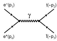
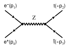
In lowest order perturbation theory the process can be illustrated by the two Feynman diagrams of Fig. 2.1.
For convenience we introduce the following abbreviations:
| (2.1) | ||||
| (2.2) | ||||
| (2.3) |
In the Feynman gauge the matrix elements corresponding to Fig. 2.1 are:
| (2.4) | ||||
| (2.5) |
with
| (2.6) | ||||
| (2.7) |
where is the quantum number corresponding to the third component of the weak isospin, the electromagnetic charge, and the weak mixing angle.
We parametrize the radiative corrections by means of form factors. Defining the following four matrix elements
| (2.8) |
with and , the Born amplitude can be written in a compact form:
| (2.9) |
The form factors are
| (2.10) | ||||
| (2.11) | ||||
| (2.12) | ||||
| (2.13) |
Besides (2.8), we find at one-loop level three further basic matrix element structures (in the limit of vanishing electron mass):
| (2.14) |
with
| (2.15) | ||||
| (2.16) | ||||
| (2.17) | ||||
| (2.18) |
and respectively sixteen scalar form factors in total. An alternative notion uses the helicity structures,
| (2.19) |
etc., with . The interferences of these matrix elements with the Born amplitude have to be calculated. Only six of these interferences are independent, e.g. , and , 333 We are grateful to D. Bardin and P. Christova for drawing our attention to this simplification. i.e. we have the following 10 equivalences :
| (2.20) | |||||
| (2.21) | |||||
| (2.22) | |||||
| (2.23) | |||||
| (2.24) | |||||
| (2.25) | |||||
| (2.26) | |||||
| (2.27) |
In the massless limit () , only and will contribute to the cross-section, and it can be expressed in terms of the Born-like structures exclusively. We introduce the variables
| (2.28) | ||||
| (2.29) | ||||
| (2.30) |
Based on the relations (2.20 to 2.27 ) the virtual corrections can be expressed in terms of six independent, modified, dimensionless form factors :
| (2.31) | |||||
| (2.32) | |||||
| (2.33) | |||||
| (2.34) | |||||
| (2.35) | |||||
| (2.36) |
The resulting cross-section formula is:
| (2.37) | |||||
where the dimensionless form factors are
| (2.38) | |||||
| (2.39) |
and , . The are defined so that double counting for the Born contributions is avoided. The factor is conventional.
In the numerical program, helicity form factors are calculated as well. They are defined as follows:
| (2.40) | |||||
| (2.41) | |||||
| (2.42) | |||||
| (2.43) |
At the end of this introductory section, we would like to give the relation of our form factors to those used in the literature for pair production of massless fermions. In that case, only the four form factors contribute. They have to replace, in the massless limit, the form factors and , which are conventionally used to renormalize the muon decay constant and the weak mixing angle and are precisely defined in [22, 23]. We rewrite the matrix element in such a way that it gives exactly the Born amplitude (2.5) when the four form factors are set equal to 1:
| (2.44) |
From here, it is easy to derive the relations between the form factors in an (L,R) or (1,5) basis and , respectively:
| (2.45) | ||||
| (2.46) | ||||
| (2.47) | ||||
| (2.48) |
Three process-dependent effective weak mixing angles and the weak coupling strength are obtained by inverting these relations:
| (2.49) | |||||
| (2.50) | |||||
| (2.51) | |||||
| (2.52) |
For the simplest approximations with factorizing, universal weak corrections, the , , and become equal, real and constant (independent of process and kinematics); for more details see for instance the discussion of the weak corrections in [15, 16] and references therein. There, also the important influence of higher order corrections is considered.
3 Virtual Corrections
The virtual corrections come from self-energy insertions, vertex and box diagrams, and from renormalization. A complete list of the contributing diagrams may be found in [19]. By means of the package DIANA [24, 25, 26] we generated useful graphical presentations of the diagrams and the input for subsequent FORM [27, 28] manipulations. With the DIANA output (FORM input), we performed two independent calculations of the virtual form factors, both using the ’t Hooft–Feynman gauge.
For the final numerical evaluations we used two Fortran packages: FF [29] and LoopTools [30]. Both have been taken from the corresponding homepages, and LoopTools was slightly adapted: one infrared was added and the was used only for photon mass .
In the package FF, the Passarino–Veltman tensor decomposition of the amplitudes [31] is defined in terms of the external momenta of the diagrams, while in LoopTools this decomposition is performed in terms of internal momenta and the latter are later expressed in terms of the external ones. The resulting linear relation between the corresponding form factors is given in Appendix A. Both the ultraviolet (UV) and the infrared (IR) divergences are treated by dimensional regularization, introducing the dimension and parametrizing the infinities as poles in . The UV divergences have to be eliminated by renormalization on the amplitude level, while the IR ones can only be eliminated on the cross-section level by including the emission of soft photons. For the IR divergences we have alternatively introduced a finite photon mass, as is foreseen in FF, yielding a logarithmic singularity in this mass. Agreement to high precision was achieved for the two approaches.
Because the calculation of one-loop corrections for two-fermion production is well known, we do not present a detailed prescription of the calculations. We perform the renormalization closely following [32]. On the other hand, we want to fix some cornerstones and sketch the renormalization and show the UV-divergent parts of all the contributing diagrams, such that their cancellations can be deduced. The treatment of the IR divergences will be discussed in more detail because of the interplay with real photonic corrections. Finally, concerning the finite parts, we refer to the Fortran program topfit. We only mention that we did not perform a complete reduction of the various scalar functions to , , , and , since this is not needed for a purely numerical evaluation.
3.1 The self-energy diagrams
We have to renormalize the UV singularities of the self-energies of the photon and the boson, and also that of their mixing. Since the counter terms from wave-function and parameter renormalization must exhibit Born-like structures, it is clear from the very beginning that a cancellation of UV divergences can only occur in terms of single propagator poles. The double poles, which originally occur in the self-energy diagrams, are cancelled by mass renormalization. This we want to stress for the following, by allowing only single poles in the self-energy contributions. Thus the photon self-energy and the self-energy diagrams take the form
| (3.1) | |||||
| (3.2) |
In the – mixing diagrams, a partial fraction decomposition of the product is performed, but no subtraction:
| (3.3) | |||||
| (3.4) |
We give the UV-divergent parts of the renormalized self-energies (for definitions, see Appendix B):
| (3.5) | |||||
| (3.6) | |||||
| (3.7) |
Three families of fermions are assumed. The UV-divergent terms of the self-energies are independent of the fermion masses, but this is, of course, not true for the finite contributions.
The form factors are easily deduced from the above representations. The photon self-energy, for instance, contributes to only:
| (3.8) |
3.2 The vertex diagrams
From the initial-state vertex corrections, form factors , arise, and from the final vertices and , the latter being proportional to . There are UV divergences from the vertex diagrams in : again only Born-like amplitudes are UV-divergent.
The divergent parts of vertices with a photon or boson in the -channel, correspondingly, are:444To compactify the following formula we introduce the abbreviations: and .
| (3.9) | |||||
The explicit expressions from the initial and final photonic vertices are:
| (3.11) | |||||
| (3.12) | |||||
| (3.13) |
For the boson in the -channel we only give the sum of the initial- and final-state fermion vertices:
| (3.16) | |||||
| (3.17) |
The resulting form factors can be extracted, e.g.
| (3.18) |
3.3 The box diagrams
, and box diagrams contribute to all form factors to introduced in (2.14) to (2.18), while the box diagram contributes only to . The pure photonic box diagrams contribute only to and . Simple power counting shows that there are no UV divergences from the boxes. The IR divergences will be discussed in Section 3.5 and Appendix C.
3.4 The counter-term contributions
Finally we have to take into account the contribution from the counter terms of Appendix B, where we also introduce some of the notation to be used in the following. With these the photon exchange becomes:
| (3.19) |
Analogously, for the exchange
| (3.20) | |||||
It is again easy to collect from the above expressions the corresponding contributions to the form factors to . The contributions to, say, from the counter terms are:
| (3.21) | |||||
The resulting terms may be read off in Appendix B.
The sum of all the terms listed in the foregoing subsections for the form factors , , has been shown to finally vanish separately for the photon and the pole of the s-channel propagator:
| (3.22) |
3.5 Infrared divergences
In topfit, we have incorporated two weak libraries. One uses the package LoopTools [30], and the other one the package FF [29]. With these two options, we have a variety of internal cross checks at our disposal.
The photonic virtual corrections contain infrared divergences. They appear as singular behaviour of classes of one-loop functions. One may follow several strategies to handle them in a numerical calculation. The simplest one is to blindly give the task to the library for numerical calculation of the one-loop functions and then control the infrared stability numerically in the Fortran program. Both packages allow for this approach; LoopTools with dimensional regularization or with a finite photon mass, while FF treats loop functions with finite photon mass only.
In addition, we checked the IR stability in two ways explicitly. In the library based on FF, we simply took a small but finite photon mass and directly applied FF without simplifying any tensor functions. Several analytic checks were also performed. In the other one, we isolated in all the scalar functions the IR divergence explicitly and the cancellations with the divergences from bremsstrahlung corrections (see Section 4.3) were controlled both analytically and numerically.
In Appendix C, we fix the notation and discuss the basics of the treatment of IR divergences. In the rest of this section, we simply give a list of the divergent parts of the form factors:
From the renormalization of the fermion self-energies (wave function renormalization factors) :
| (3.23) |
From the vertex corrections (index ):
| (3.24) |
These form factors combine in the cross-section with the initial- and final-state soft photon corrections to an infrared-finite contribution. For instance, the pure photonic parts contribute only to . The resulting IR-divergent cross-section contribution in (2.37),
| (3.25) |
with
| (3.26) |
A little more involved are the box diagram contributions. As a typical example, we show the photonic box parts. The direct box gives:
| (3.27) | |||||
| (3.28) | |||||
| (3.29) |
with
| (3.30) |
From these expressions, the form factors (2.31) to (2.35) get contributions:
| (3.31) |
and all the others vanish. Analogously, from the crossed photonic box diagram:
| (3.32) | |||||
| (3.33) | |||||
| (3.34) |
with
| (3.35) |
From these expressions, the form factors (2.31) to (2.35) get contributions:
| (3.36) |
and again all the others vanish.
In Appendix C we show the relevant scalar functions explicitly.
4 Real Photonic Radiative Corrections
4.1 The three-particle phase space
The reaction
| (4.1) |
with
| (4.2) |
is the one which in reality always takes place, even if for soft photons the ‘elastic’ Born cross-section can be a good approximation without taking into account the radiated photons. Here we introduce the final-state phase-space parametrization: for convenience of notation, the top physical momenta are used here. We will not neglect the electron mass systematically, , and . Our semi-analytical integration approach with physically accessible observables as integration variables may be used to set benchmarks and to control the numerical precision to more than four digits. Their choice is constrained by the observables we want to predict, notably the angular distribution and certain cross-section asymmetries. Basically we follow the approach proposed in [33, 34] and extend the required formulae to the massive fermion case.
There is not too much found in the literature for the radiative production of massive fermion pairs. Thus, we will discuss the kinematical details with some care, since they define the integration boundaries of our numerical integration program.
In (2.1) and (2.3) we defined and for two-particle production. With the additional photon in the final state, we have to be more specific and will use the following definitions:
| (4.3) | |||||
| (4.4) |
Additionally, the following invariants will be used:
| (4.5) | |||||
| (4.6) | |||||
| (4.7) |
The squares of all three-momenta in the centre-of-mass system can be expressed in terms of a set of functions:
| (4.8) | |||||
| (4.9) | |||||
| (4.10) | |||||
| (4.11) |
where we use and the relation for .
The phase space of three particles in the final state is five-dimensional. This means that only five of the ten scalar products (those introduced already: , plus ) built from the five momenta are independent. In fact, the following relations hold
| (4.12) | |||||
| (4.13) |
We use the first of relations (4.12) in order to substitute everywhere in favour of as already done in (4.9). Since we do not consider transversally polarized initial particles, an integration of the cross section over the corresponding rotation angle is trivially giving a factor and we are left with four non-trivial phase space variables.
For the calculation of the forward–backward asymmetry, the angle between the three-momenta of and is used, in accordance with (4.3). Further, the energies , , and are ‘good’ variables. As mentioned before, they can be expressed in terms of the invariants and :
| (4.14) | |||||
| (4.15) | |||||
| (4.16) |
The scattering angle in the centre-of-mass system may now be expressed by invariants:
| (4.17) |
As will be seen later, the two invariants and also describe the angles between any pair of final-state particles. Therefore, we choose them to parametrize the phase space. Finally, the fourth integration variable will be the azimuthal angle of the photon .
The coordinate system is chosen such that the moves along the axis and the beam axis is in the – plane. The four-momenta of all particles can then be written as follows:
| (4.18) | |||||
| (4.19) | |||||
| (4.20) | |||||
| (4.21) | |||||
| (4.22) |
The and are the azimuthal and polar angles of the photon. The expression for (and also that for ) can be obtained from ,
| (4.23) |
and again depends only on and . The differential bremsstrahlung cross section (4.2) takes the form
| (4.24) |
In the last step, dimensionless variables are introduced:
| (4.25) | |||||
| (4.26) | |||||
| (4.27) |
The integration boundaries are either trivial ( and ) or can be found from the condition that the three three-vectors form a triangle with the geometrical constraint . The four integration variables vary within the following regions:
| (4.28) | |||||
| (4.29) | |||||
| (4.30) | |||||
| (4.31) |
If the order of integrations over and is interchanged, their boundaries are
| (4.32) | |||||
| (4.33) |


The kinematic regions of and are shown in Fig. 4.1(a) for massless () and in Fig. 4.1(b) for massive () final fermions. At the kinematic boundaries, the three-momenta are parallel. Further, there are three special points where exactly one of the three three-momenta vanishes
| (4.34) | |||||
| (4.35) | |||||
| (4.36) |
At point the soft photons are located. Section 4.3 is devoted to their treatment. The () are at rest in (). In the massless case, , the three points and are located at the corners of the kinematic triangle, . From (4.14)–(4.16) it follows that the photon energy is maximal at the left edge, coinciding with the -axis; the fermion energy is maximal at the lower edge, coinciding with the -axis; and finally the energy of the anti fermion is maximal at the third edge.
4.1.1 Energy cuts
Cuts on the energy of the final state particles are of importance for two reasons: they are being applied in the experimental set-ups, and for the photon we have to identify the soft photon terms in order to combine them with virtual corrections for a finite net elastic cross section. The lower hard photon energy (being also the upper soft photon energy) is
| (4.37) |
All three energy cuts are deduced from (4.14) to (4.16). The photon energy is related to by
| (4.38) |
and the limits to be imposed are
| (4.39) |
Constraining the fermion energies leads to cuts on :
| (4.40) |
All the energy cuts are independent of the mass of the final fermions and of . They are illustrated in Fig.4.1. From (4.40) it can be seen that the derivatives of the kinematic border at points and in Fig. 4.1(b) (for their definitions see (4.34) and (4.35)) are and .
4.1.2 Angular cuts
The scattering angle
is the angle between and . This angle is one of the integration variables and is constrained directly:
| (4.41) |
Additional angular cuts deserve a study of the () parameter space. To be definite, we will always consider the kinematic bound of for an arbitrarily chosen value of .
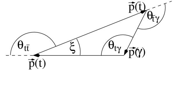
The directions of the final-state particles define three angles , , and ; as shown In Fig. 4.2. The acollinearity angle is defined by
| (4.42) |
The condition restricts the events to a Born-like kinematics: the fermions are back to back and only soft photons or photons collinear to one of the final fermions are allowed. Using the above formulae, the acollinearity angle is expressed in terms of the invariants and :
| (4.43) |
Equation (4.43) can readily be derived considering the scalar product or alternatively the triangle of the three-momenta of the final particles in Fig. 4.2, with account of the relations (4.11) between functions and absolute values of three-momenta.


For massless fermions, Eq. (4.43) is much simpler and describes a hyperbola with a symmetry axis rotated by an angle of relative to the axis. The kinematic regions for different values of the acollinearity angle are shown in Fig. 4.3. All lines intersect at the points and . For moderate cuts on the maximum acollinearity angle, the kinematic area is only constrained for values of above the point , i.e. for . In this case only the lower bound of is changed. The constraint to the kinematic region acts in a way similar to a cut to hard photons. This is clear from the topology of events with high acollinearity: the fermion and anti fermion fly approximately in one direction and must recoil against a hard photon. For stronger acollinearity cuts, constraints of the kinematic area arise also for values of below the point . In this case the allowed range for splits in two regions. The first region extends from the lower kinematic border to the smaller solution of (4.43), while the second region extends from the larger solution of (4.43) to the upper kinematic border.
The analytic treatment of the acollinearity cut for the massless case was also discussed in [35, 36, 23, 37].
In a similar way as explained for the acollinearity angle, the two angles and can be expressed in terms of the two invariants and :
| (4.44) | |||||
| (4.45) |
Although physically the situation for a cut on is equivalent to a cut on , the symmetry is broken because we had to make a choice between and . The constraint on leads to a quadratic equation in and , while that for is quadratic in and of fourth order in . In the massless case, the constraints to become a bilinear equation in and , describing a hyperbola with a symmetry axis, which is rotated by an angle relative to the axis. The massless limit of (4.45) leads to a constraint on , which is linear in and quadratic in , describing a hyperbola with a symmetry axis, which is rotated by an angle of relative to the axis.


The kinematic regions for different values of the angle are shown in Fig. 4.4. All lines intersect at the points and . The exclusion of events with small angles excludes regions near the edge . These kinematic regions correspond to events with large anti fermion energies, (compare Fig. 4.1). Technically, a constraint of the angle from below changes the upper bound of in the kinematic region for a fixed . The lower bound of is unchanged by this cut.


Finally, the kinematic regions for different values of the angle are shown in Fig. 4.5. All lines intersect at the points and . The exclusion of events with small angles excludes regions near the axis. These kinematic regions correspond to events with large fermion energies, (compare Fig. 4.2). Technically, a constraint of the angle from below affects the kinematic region only for some below a certain value. For these and for massless fermions, the integration region of is split into two regions. The first region extends from the lower kinematic border to the smaller solution of (4.45), and the second one extends from the larger solution of (4.45) to the upper kinematic border. For massive fermions, the cutting out of small angles changes only the lower bound of as far as is below the point . For a harder cut on , the kinematic region is also affected for values of , larger than the coordinate of the point . For a fixed and finite , two regions of near the kinematic border are then allowed, while some region in the “middle” is cut out by the constraint. This is similar to the situation in the massless case.
4.2 Radiative differential cross sections
For massless fermions, typically a threefold analytical integration of the radiative contributions to fermion pair production with realistic cuts may be performed, see [36, 23, 35] and references quoted therein. For massive pair production, everything becomes non-trivial and, in the end, we decided to perform only the first integration analytically, that over . This leaves three integrations at most for a numerical treatment. Our practice proved that the accuracy and speed are absolutely satisfactory for our needs of calculating benchmarks and physics case studies.
For this reasons, and in order to make everything well-defined, we now have to collect the singly analytically integrated contributions to be used in a subsequent numerical calculation.
We will use a notation for the couplings with some flexibility not needed in the Born case:
| (4.46) | |||||
| (4.47) | |||||
| (4.48) | |||||
| (4.49) | |||||
where we use , , , and and
| (4.50) | |||||
| (4.51) |
With these conventions, the Born cross section becomes
| (4.52) |
The cross section for subdivides in the gauge-invariant subsets of initial-state radiation, final-state radiation and the interference between them. Explicit expressions for the totally differential cross section may be found in [37]. The integration over is not too complicated and in fact we could simply use existing tables of integrals [33, 34, 37]. This first integration is unaffected by the cuts discussed and has to be performed with an exact treatment of both and .
The cross section for initial-state radiation after the integration over is
| (4.53) | |||||
with
| (4.54) | |||||
| (4.55) | |||||
| (4.56) | |||||
| (4.57) | |||||
The cross section for final-state radiation after the integration over is
| (4.58) | |||||
with
| (4.59) |
The cross section for the interference between initial- and final-state radiation after the integration over is
| (4.60) | |||||
4.3 Soft photon corrections
The four-dimensional integration of the bremsstrahlung contributions is divergent in the soft-photon part of the phase-space and is treated in dimensions. One starts from a reparametrization of the photonic phase-space part with Born-like kinematics for the matrix element squared. To obtain a soft photon contribution we have to take the terms of the bremsstrahlung amplitude without in the numerators. In this limit, approaches and the soft contribution to the differential cross section takes the form
| (4.61) |
with
| (4.62) | |||||
and
| (4.63) | |||||
The scalar products have to be taken according to Born kinematics, i.e. the expressions (4.6) and (4.7) become
| (4.64) | |||||
| (4.65) | |||||
| (4.66) | |||||
| (4.67) |
From here we see that is constructed to be independent of . Substitute now, with , ,
| (4.68) | |||||
We introduce the abbreviation for the infrared divergence
| (4.69) |
The infrared divergence can also be regularized by introducing a finite photon mass :
| (4.70) |
The last integral over is trivial for the products and , since they contain only one angle; one may thus identify either or . In the initial–final interference, one may introduce a Feynman parameter
| (4.71) |
with
| (4.72) |
Then, and identify now . Further,
| (4.73) | |||||
| (4.74) |
The final result is
| (4.75) |
with
| (4.76) | |||||
| (4.77) | |||||
| (4.78) | |||||
and
| (4.79) | |||||
| (4.80) |
and analogue definitions for . We calculate the finite interference part given in (4.78) numerically, but have shown the agreement with Eq. (3.64) of [38]:
| (4.81) | |||||
5 Results
In this section we present the numerical results of the electroweak
one-loop calculation to the process . We have performed a
fixed-order
calculation, i.e. no higher order corrections such as
photon exponentiation have been taken into account.
For the numerical evaluation we assume the following input values [20, 19, 18]:
| (5.6) |
Two packages, namely FF [29] and LoopTools
[30] have been used for the numerical evaluation of the loop
integrals.
In Fig. 5.1, we present the differential cross section for various generic values of .

It can be seen that for rather high
centre-of-mass
energies the characteristic features of a massive
fermion pair production become less prominent. At TeV
the differential cross section of electroweak radiative corrections
starts to exhibit collinear mass singularities at the
edges of phase
space.
Those are cured by applying
a cut on .
In general it can be
seen that the effects of radiative corrections are more dramatic for
top-pairs produced close to the direction of the beam. For the TESLA
range of centre-of-mass energies, backward scattered top quarks give
rise to slightly larger corrections than forward scattered ones [19]. For
higher energies this effect is more or less washed out.
In Table 5.1 to 5.3 we present a complete set of form
factors entering the cross-section calculation. The form factors given
correspond to the minimal set of independent form factors possible
for a two-to-two process with two massless and two massive fermions in
the initial and final state respectively, and are defined with respect
to
the ‘naturally’ arising form factors in Eq. (2.31). For
completeness we also give the corresponding Born form factors. The
numerical values given are obtained for a characteristic
centre-of-mass
energy of GeV and a fixed scattering angle
.
| f.f. | Born | weak 1-loop contributions | ||
|---|---|---|---|---|
| Re | Im | Re | Im | |
| f.f. | Born | weak 1-loop contributions | ||
|---|---|---|---|---|
| Re | Im | Re | Im | |
| f.f. | Born | weak 1-loop contributions | ||
|---|---|---|---|---|
| Re | Im | Re | Im | |
In Fig. 5.2 we present the total integrated cross section as a function of . From the previous discussion it is clear that the effect of radiative corrections is less dramatic in the total cross section, since the effects above and below the Born cross section are averaged out.

Finally the forward–backward asymmetry of the total integrated cross
section can serve as a good observable to determine the effects of
radiative corrections. Towards higher energies, the effects become
distinctively.

In summary our calculation shows that for the next generation of linear colliders with centre-of-mass energies above = 500 GeV, electroweak radiative corrections modify the differential as well as the integrated cross section within the experimental precision of a few per mille. The package topfit provides the means to calculate those corrections and allows predictions for various realistic cuts on the scattering angle as well as on the energy of the photon.
Acknowledgements
J.F. and A. L. would like to thank DESY Zeuthen for invitations and all authors thank the Heisenberg-Landau projekt ‘New methods of computing massive Feynman integrals and mass effects in the Standard Model’ for financing visits to Dubna.
Appendices
A Translation of Tensor Decompositions
On the left-hand side we give the Passarino-Veltman functions, used in [29], according to the tensor decomposition of Feynman diagrams with respect to external momenta as systematically introduced in [31]. On the right-hand side we follow the corresponding notation in the LoopTools package [30], with . There are also sign differences reflecting different notions of metrics.
| (A.1) | |||||
| (A.2) | |||||
| (A.3) | |||||
| (A.4) | |||||
| (A.5) | |||||
| (A.6) | |||||
| (A.7) | |||||
| (A.8) | |||||
| (A.9) | |||||
| (A.10) | |||||
| (A.11) | |||||
| (A.12) | |||||
| (A.13) | |||||
| (A.14) | |||||
| (A.15) | |||||
| (A.16) | |||||
| (A.17) |
B Renormalization
A detailed formulation of renormalization of fermion pair production can be found in various textbooks, e.g. [39]. To complete the documentation of our calculation we present some relations resulting from the application of an on-mass-shell renormalization, closely following [32]. They had been used to derive the formulae given in Section 3.
After the renormalization of the boson self-energies: we have to use the following expressions:
| (B.1) | |||||
| (B.2) | |||||
| (B.3) |
The divergent parts of those renormalized self-energies were given in (3.7). For the mixing angle renormalization and are needed:
| (B.4) |
Among the free parameters of the theory we have, only one coupling constant , using
| (B.5) |
The electric charge renormalization differs in pure QED and electroweak theory
| (B.6) | |||||
| (B.7) | |||||
| (B.8) |
The wav-function renormalization factor is obtained from the fermion self-energy , with
| (B.9) |
The resulting factor is:
| (B.10) | |||||
For QED, the axial terms vanish, of course.
Explicitly, the UV-divergent parts are given by :
| (B.11) | |||||
| (B.12) | |||||
| (B.13) | |||||
| (B.14) |
with denoting the isospin partner of .
The above relations define the complete renormalization procedure needed for our reaction. A vertex renormalization, e.g. resulting from terms such as in the Lagrangian, traces back to and . Explicit formulae may be found in the Fortran code [17].
C Infrared Divergences
The conventions of the one-loop functions and related ones are those used in the package LoopTools [30]. In particular the normalization of the one-loop integration is used as in the following simplest example:
| (C.1) | |||||
In the Fortran program, we leave the treatment of IR divergences to the packages used for the calculation of one-loop integrals. Additionally, we checked analytically their cancellation. For this purpose, we isolated them in the few IR-divergent scalar integrals contributing to the process .
One-loop infrared divergences are due to the exchange of a photon between two massive particles, which occur also as external (on-shell) ones.
Wave function renormalization yields IR-divergent contributions and , the on-mass-shell derivatives of and (w.r.t. the external momentum squared). From 555In FF, there is no foreseen, while in LoopTools this function was numerically unstable for . This might be improved now. With the representation
| (C.2) |
one arrives at
| (C.3) | |||||
The UV divergences cancel at the right-hand side and the IR divergence is traced back to . We mention for completeness that the similar function , arising from the charged current self-energy with a massless neutrino, is finite.
An explicit calculation gives
| (C.4) | |||||
| (C.5) |
Assigning the loop-momentum to the photon line in the initial- and final-state vertex diagrams ensures that the divergent part is exclusively contained in one scalar three-point function :
with
| (C.7) |
The finite, small photon mass is defined according to (4.70).
Finally, IR-divergent functions from the photonic box diagrams, , , , and , have to be considered. We indicate for the direct two-photon box, shown in Fig. .4, how the singularities can be isolated.
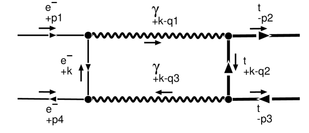
The key ingredient for this method [31] is the following identity:
For , evidently the numerator of the first of the three terms makes it an IR-finite contribution and the other two are functions. To demonstrate more explicitely the procedure we select the above diagram (see Fig. .4) and obtain (see also [40]):
| (C.9) | |||||
Only one scalar function has to be calculated, and in the limit of vanishing we find
| (C.10) |
From the crossed box diagram, we get another function, , with in Eq. (C.10) replaced by . When combining virtual and soft corrections, the singularities of these functions are cancelled against the divergent parts of (4.78).
The vector and tensor functions may be treated quite similarly:
| (C.11) | |||||
| (C.12) | |||||
To cross-check the result, we isolated the IR-divergent parts also with another approach, where the tensor integrals are reduced to scalar ones by means of recurrence relations [41, 42]. The divergent contributions hidden in the tensor integrals manifest themselves in the form of the three IR-divergent scalar functions introduced above, namely (C.5) for self-energies, (C) for vertices, and (C.10) for boxes, correspondingly.
References
- [1] E. H. Simmons, “The top quark: Experimental roots and branches of theory”, Boston Univ. preprint BUHEP 02-39 (2002), to appear in: M. Erdmann et al. (eds.), Proc. of the 14th Topical Conference on Hadron Collider Physics, Sept/Oct 2002, Karlsruhe, Germany (HCP2002), hep-ph/0211335.
- [2] ECFA/DESY LC Physics Working Group (E. Accomando et al.), Phys. Rept. 299 (1998) 1, hep-ph/9705442.
- [3] ECFA/DESY LC Physics Working Group (J. Aguilar-Saavedra et al.), “TESLA Technical Design Report Part III: Physics at an Linear Collider”, preprint DESY 2001–011 (2001), hep-ph/0106315.
- [4] American Linear Collider Working Group (T. Abe et al.), “Linear collider physics resource book for Snowmass 2001”, Fermilab preprint FERMILAB-PUB-01-058-E (2001), hep-ex/0106055, hep-ex/0106056, hep-ex/0106057, hep-ex/0106058.
- [5] A. Biernacik, K. Cieckiewicz, and K. Kolodziej, Eur. Phys. J. C20 (2001) 233–237, hep-ph/0102253.
- [6] K. Kolodziej, Eur. Phys. J. C23 (2002) 471–477, hep-ph/0110063.
- [7] A. Biernacik and K. Kolodziej, “Top quark pair production and decay at linear colliders: Signal vs. off resonance background”, to appear in: J. Blümlein et al. (eds.), Proc. of 6th Int. Symp. on Radiative Corrections: Application of Quantum Field Theory Phenomenology (RADCOR 2002) and 6th Zeuthen Workshop on Elementary Particle Theory (Loops and Legs in Quantum Field Theory), Kloster Banz, Germany, 8-13 Sep 2002, hep-ph/0210405.
- [8] M. L. Nekrasov, Phys. Lett. B545 (2002) 119–126, hep-ph/0207215.
- [9] S. Dittmaier and M. Roth, Nucl. Phys. B642 (2002) 307–343, hep-ph/0206070.
- [10] J. Fujimoto and Y. Shimizu, Mod. Phys. Lett. 3A (1988) 581.
- [11] F. Yuasa et al., Prog. Theor. Phys. Suppl. 138 (2000) 18–23, hep-ph/0007053.
- [12] W. Beenakker, S. van der Marck, and W. Hollik, Nucl. Phys. B365 (1991) 24–78.
- [13] W. Hollik and C. Schappacher, Nucl. Phys. B545 (1999) 98–140, hep-ph/9807427.
- [14] D. Bardin, L. Kalinovskaya, and G. Nanava, “An electroweak library for the calculation of EWRC to within the CalcPHEP project”, Dubna preprint JINR E2–2000–292 (2000), hep-ph/0012080, v.2 (12 Dec 2001).
- [15] D. Bardin et al., “Electroweak working group report”, in Reports of the Working Group on Precision Calculations for the Resonance, report CERN 95–03 (1995) (D. Bardin, W. Hollik, and G. Passarino, eds.), pp. 7–162, hep-ph/9709229.
- [16] Two Fermion Working Group (M. Kobel et al.), “Two-fermion production in electron positron collisions”, in Reports of the working groups on precision calculations for LEP2 physics, Proc. of the Monte Carlo Workshop, Geneva, 1999-2000, report CERN 2000-09-D (2000) (S. Jadach, G. Passarino, and R. Pittau, eds.), pp. 269–378, hep-ph/0007180.
-
[17]
J. Fleischer, A. Leike, T. Riemann, and A. Werthenbach, Fortran program topfit.F v.0.91 (06 March 2002),
http://www-zeuthen.desy.de/~riemann/. - [18] J. Fleischer, A. Leike, T. Riemann, and A. Werthenbach, “Status of electroweak corrections to top pair production”, preprint DESY 02–203 (2002), to appear in Proc. of the Int. Workshop on Linear Colliders (LCWS 2002), 26–30 Aug 2002, Jeju Island, Korea, hep-ph/0211428.
- [19] J. Fleischer, T. Hahn, W. Hollik, T. Riemann, C. Schappacher, and A. Werthenbach, “Complete electroweak one-loop radiative corrections to top-pair production at TESLA: A comparison”, TESLA note LC-TH-2002-002 (2002), contribution to the second workshop of the extended ECFA/DESY study “Physics and Detectors for a 90 to 800 GeV Linear Collider”, 12-15 April 2002, Saint-Malo, France, hep-ph/0202109.
- [20] J. Fleischer, J. Fujimoto, T. Ishikawa, A. Leike, T. Riemann, Y. Shimizu, and A. Werthenbach, “One-loop corrections to the process including hard bremsstrahlung”, in Second Symposium on Computational Particle Physics (CPP, Tokyo, 28–30 Nov 2001), KEK Proceedings 2002-11 (2002) (Y. Kurihara, ed.), pp. 153–162, hep-ph/0203220.
- [21] A. Andonov et al., “Update of one loop corrections for , first run of CalcPHEP system”, preprint CERN-TH/2001-308 (2001), CERN-TH/2002-068 (2002), hep-ph/0207156.
- [22] D. Bardin, M. Bilenky, G. Mitselmakher, T. Riemann, and M. Sachwitz, Z. Phys. C44 (1989) 493.
- [23] D. Bardin, P. Christova, M. Jack, L. Kalinovskaya, A. Olchevski, S. Riemann, and T. Riemann, Comput. Phys. Commun. 133 (2001) 229–395, hep-ph/9908433.
- [24] M. Tentyukov and J. Fleischer, Comput. Phys. Commun. 132 (2000) 124–141, hep-ph/9904258.
-
[25]
M. Tentyukov and J. Fleischer,
“DIANA, a program for Feynman diagram evaluation”, hep-ph/9905560, see also
http://www.physik.uni-bielefeld.de/~tentukov/diana.html. - [26] J. Fleischer and M. Tentyukov, “A Feynman diagram analyser DIANA: Graphic facilities”, in: P. Bhat and M. Kasemann (eds.), Proc. of the VIIth Int. Workshop ACAT 2000, Batavia, USA, 16-20 Oct. 2000, AIP Conference Proceedings (Melville, New York, 2001), vol. 583, p. 193, hep-ph/0012189.
- [27] J. Vermaseren, “Symbolic manipulation with FORM” (Computer Algebra Nederland, Amsterdam, 1991).
- [28] J. Vermaseren, “New features of FORM”, math-ph/0010025.
- [29] G. van Oldenborgh, Comput. Phys. Commun. 66 (1991) 1–15; http://www.xs4all.nl/ gjvo/.
- [30] T. Hahn and M. Perez-Victoria, Comput. Phys. Commun. 118 (1999) 153–165; http://www.feyn-arts.de/looptools, hep-ph/9807565.
- [31] G. Passarino and M. Veltman, Nucl. Phys. B160 (1979) 151.
- [32] J. Fleischer and F. Jegerlehner, Phys. Rev. D23 (1981) 2001–2026.
- [33] D. Bardin and N. Shumeiko, Nucl. Phys. B127 (1977) 242.
- [34] G. Passarino, Nucl. Phys. B204 (1982) 237–266.
- [35] G. Montagna, O. Nicrosini, and G. Passarino, Phys. Lett. B309 (1993) 436–442.
- [36] P. Christova, M. Jack, and T. Riemann, Phys. Lett. B456 (1999) 264–269, hep-ph/9902408.
- [37] M. Jack, “Semi-analytical calculation of QED radiative corrections to with special emphasis on kinematical cuts to the final state”, preprint DESY-THESIS 2000-030 (August 2000), hep-ph/0009068.
- [38] W. Beenakker, “Electroweak corrections: Techniques and applications”, Ph.D. thesis, Univ. Leiden, 1989.
- [39] M. Böhm, A. Denner, and H. Joos, Gauge Theories of the Strong and Electroweak Interaction (Teubner, Stuttgart, 2001).
- [40] J. Fleischer, F. Jegerlehner, and M. Zralek, Z. Phys. C42 (1989) 409.
- [41] O. V. Tarasov, Phys. Rev. D54 (1996) 6479–6490, hep-th/9606018.
- [42] J. Fleischer, F. Jegerlehner, and O. V. Tarasov, Nucl. Phys. B566 (2000) 423–440, hep-ph/9907327.