Geometry of Reggeized amplitudes from AdS/CFT

Abstract:

String theory has long ago been initiated by the quest for a theoretical explanation of the observed high-energy “Reggeization” of strong interaction amplitudes. In terms of quantum field theory, it is the so-called “soft” regime, where the coupling constant is expected to be large and thus perturbative calculations inadequate. However, since then, no convincing derivation of the link between gauge field theory at strong coupling and string theory has come out. This 35-years-old puzzle is thus still unsolved. We discuss how modern tools like the AdS/CFT correspondence give a new insight on the problem by applying it to two-body elastic and inelastic scattering amplitudes. We obtain a geometrical interpretation of Reggeization and its relation with confinement in gauge theory.

1 Introduction

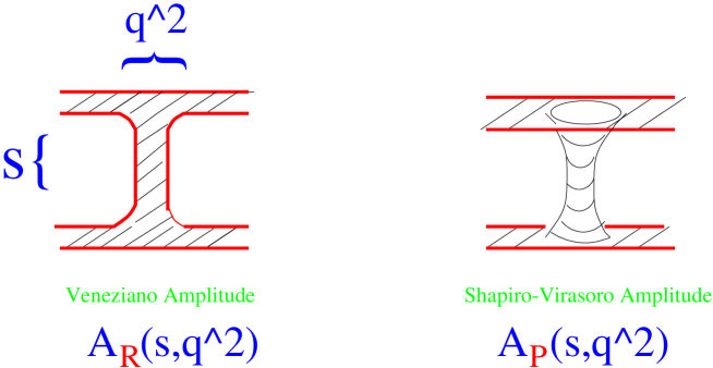
Figure 1: “Duality diagrams” for two-body inelastic and elastic amplitudes.

It is well-known that string theory started from the proposal of scattering amplitudes which may grasp the two major structures of soft interaction phenomenology for $2\to 2$ reactions in a condensed form: resonances and Regge poles. Two types of amplitudes were proposed for four-point amplitudes. The Veneziano amplitude corresponds to Reggeon exchanges with non-vacuum quantum numbers, i.e. inelastic two-body reaction amplitudes, and the Shapiro-Virasoro amplitude corresponds to Pomeron exchange with vacuum quantum numbers, i.e. elastic amplitudes. These amplitudes have been conveniently represented by “duality diagrams”, see Fig.1. In the representation of the Veneziano amplitude in terms of quark lines, $q\bar{q}$ intermediate states in the direct $s$-channel correspond to the resonances, and $q\bar{q}$ intermediate states in the exchanged $s$-channel to Regge poles, where $s,t$ are the well-known Mandelstam variables. The quark lines are to be considered as boundaries of a surface bearing no quantum numbers, as can be seen for the representation of the Shapiro-Virasoro amplitude corresponding to no quantum nmber exchange.

Quite amazingly, this representation found its justification in terms of string theory. The “duality diagram” representation of Fig. 1 can be mapped into the fusing and splitting of strings. More precisely, the Veneziano and Shapiro-Virasoro amplitudes are topologically related to open and closed tree-level string respectively. This topological relation can be more formally expressed in string theory by the invariance of amplitudes with respect to deformations of the world sheet spanned by the interacting string, and by its conformal invariant properties. After a generalization of dual amplitudes has been found for multiparticle amplitudes, this raised the hope to find both a theoretically consistent theory of strong interactions and a calculation procedure using the perturbative topological expansion of string amplitudes [1].

However, despite many efforts during years, no widely recognized progress has been done in the string theory of strong interaction amplitudes. Moreover, after the discovery of QCD as the gauge field theory of quarks and gluons and its validity for a quantitative description of many “hard” scattering processes, there remained little hope that a string theory of strong interactions could take place. Indeed, even before the discovery of QCD, major theoretical obstacles to the formulation of a consistent string theory of strong intractions were being raised. Let us give a non exhaustive list of problems.

The conformal anomaly of string theories in Minkowski $D$-dimensional space leads to the limitation $D=26,10$ for respectively bosonic and super strings in flat space. More generally, the requirement of conformal and diffeomorphism invariance imposes stringent constraints on the space in which the string moves.

Zero mass gauge and gravitational fields appear in the string spectra of asymptotic states. Consistent string theory, when considered in flat target space, contains (in general) gauge group and gravitational fields and degrees of freedom. They are thus more suitable for a stringy approach of grand unified theories, than for strong interactions and the confinement problem, characterized by the absence of asymptotic zero mass states in the theory.

To these difficulties, new ones have been added after the discovery of QCD. Let us list three among the main questions (at least those concerning the scattering of two particles):

• Can we find a consistent picture of the Reggeization of high-energy amplitudes when QCD enters its strong coupling regime?. Even knowing the QCD lagrangian, it has not been possible to derive from it high-energy amplitudes in the soft interaction case. Lattice calculations have been useful for investigations at low energy but are seemingly hopeless in the kinematical domain of high energies.

• Where are “hard” interactions recovered in a string theory framework? String world sheets are suitable objects for the description of “soft” phenomena due to their extended structure in space and time. It is more intricate to show off in string theory the “hard” structure visible in short-time interactions.

• Can we elaborate a suitable string theory which could coherently describe the properties of gauge fields?. The degrees of freedom and the symmetries of a gauge field theory are much different from those commonly found for string theories. the matching of these two require non trivial constraints as recognized in particular in Ref.[2].

To the first of these three questions, the recently proposed duality corespondence between certain string and certain gauge field theories gives new and reliable answers. It seems that the second one can find some interesting clues also in the same framework [3]. we will focus here upon the third one, namely the understanding of Regge two-body amplitudes in gauge field theories at strong coupling in terms of the AdS/CFT duality. This question has been the subject of an approach [4, 5, 6, 7] which I will now develop.

The plan of the present review is the following: in section 2, we will give a brief account of the AdS/CFT dual correspondence, focusing on aspects relevant for our study. In section 3, we will explain the formalism using the classical approximation and minimal surfaces for the determination of the AdS duals of two-body scattering amplitudes. We successively apply it to quark (anti)quark, dipole-dipole elastic scattering and finally inelastic dipole-dipole scattering. Next in 4, we will develop a semi-classical approximation, improving the previous method by computing the fluctuation factor around the minimal surface solution. A final section 5 is devoted to a summary and conclusion about the geometrical nature of Reggeization in the confining AdS dual backgrounds.

2 String/Gauge fields Duality

The AdS/CFT correspondence [8] has many interesting formal and physical facets. Concerning the aspects which are of interest for our problem, it allows one to find relations between gauge field theories at strong coupling and string gravity at weak coupling in the limit of large number of colours ($N_{c}\!\to\!\infty$). It can be examined quite precisely in the AdS₅/CFT₄ case which conformal field theory corresponds to $SU(N)$ gauge theory with ${\cal N}\!=\!4$ supersymmetries.

Some existing extensions to other gauge theories with broken conformal symmetry and less or no supersymmetries will be valuable for our approach, since they lead to confining gauge theories which are more similar to QCD. Indeed, one important question is to examine to what extent confinement plays a rôle in the Reggeization of amplitudes. Our aim is thus to investigate the possible realization and origin of Reggeization of two-body amplitudes in such theories and what are the difference appearing with the original AdS₅/CFT₄ case.

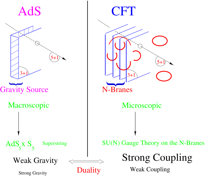
Figure 2: AdS₅/CFT₄ duality correspondence.

Let us recall the canonical derivation leading to the AdS₅ background [9], see Fig.2. One starts from the (super)gravity classical solution of a system of $N\ D_{3}$-branes in a $10\!-\!D$ space of the (type IIB) superstrings. The metrics solution of the (super)Einstein equations read

$$ds^{2}=f^{\!-\!1/2}(\!-\!dt^{2}\!+\!\sum_{1\!-\!3}dx_{i}^{2})\!+\!f^{1/2}(dr^{2}\!+\!r^{2}d\Omega_{5})\ ,$$ (1)

where the first four coordinates are on the brane and $r$ corresponds to the coordinate along the normal to the branes. In formula (1), one defines

$$f=1+\frac{R^{4}}{r^{4}}\ ;\ \ \ \ \ R=4\pi g^{2}_{YM}\alpha^{\prime 2}{N}\ ,$$ (2)

where $g^{2}_{YM}{N}$ is the ‘t Hooft-Yang-Mills coupling and $\alpha^{\prime}$ the string tension.

One considers the limiting behaviour considered by Maldacena, where one zooms on the neighbourhood of the branes while in the same time going to the limit of weak string slope $\alpha^{\prime}.$ The near-by space-time is thus distorted due to the (super) gravitational field of the branes. One goes to the limit where

$$\ R\ fixed\ ;\frac{\alpha^{\prime}(\to 0)}{r(\to 0)}\to z\ fixed\ .$$ (3)

This, from the second equation of (2) obviously implies

$${\alpha^{\prime}\to 0}\ ,\ g^{2}_{YM}{N}\sim\frac{1}{\alpha^{\prime 2}}\to\infty\ ,$$ (4)

i.e. both a weak coupling limit for the string theory and a strong coupling limit for the dual gauge field theory. By reorganizing the two parts of the metrics one obtains

$$ds^{2}={\frac{1}{z^{2}}(-dt^{2}+\sum_{1-3}dx_{i}^{2}+dz^{2})}+{R^{2}d\Omega_{5}}\ ,$$ (5)

which corresponds to the AdS₅ $\times\ {S_{5}}$ background structure, ${S_{5}}$ being the 5-sphere. More detailed analysis shows that the isometry group of the 5-sphere is the geometrical dual of the ${\cal N}\!=\!4$ supersymmetries. More intricate is the quantum number dual to $N_{c},$ the number of colours, which is the invariant charge carried by the Ramond-Ramond form field.

In the case of confining backgrounds, an intrinsic scale breaks conformal invariance and is brought in the dual theory through e.g. a geometrical constraint. For instance in [10] a proposal was made that a confining gauge theory is dual to string theory in an $AdS_{BH}$ black hole (BH) background

$$ds^{2}_{BH}=\frac{16}{9}\frac{1}{f(z)}\frac{dz^{2}}{z^{2}}+\frac{\eta_{\mu\nu}dx^{\mu}dx^{\nu}}{z^{2}}+\ldots$$ (6)

where $f(z)=z^{2/3}(1-(z/R_{0})^{4})$ and $R_{0}$ is the position of the horizon. We will use this background to study the interplay between the confining nature of gauge theory and its reggeization properties. Actually the qualitative arguments and approximations should be generic for most confining backgrounds, as already discussed in Ref. [12]. For instance, other geometries for (supersymmetric) confining theories [13, 14] have been discussed in this respect. They have the property that for small $z$, i.e. close to the boundary, the geometry looks like $AdS_{5}\times S^{5}$ (in [14] up to logarithmic corrections related to asymptotic freedom) giving a coulombic $q\bar{q}$ potential. For large $z$ the geometry is effectively flat. In all cases there is a scale, similar to $R_{0}$ above, which marks a transition between the small $z$ and large $z$ regimes.

In order to illustrate the way one formulates the AdS/CFT correspondence in a context similar to QCD, let us consider the example of the vacuum expectation value (vev) of Wilson lines in a configuration parallel to the time direction of the branes. This configuration allows a determination of the potential between colour charges [15]. The rôle of colour charges in the fundamental representation is played by open string states elongated between a stack of $N_{c}$ $D_{3}$ branes on one side and one $D_{3}$ brane near the boundary of AdS space (cf. [9]).

Figure 3: Exemple of minimal surfaces with Wilson line boundaries.

One writes

$$\langle e^{iP\int_{C}\vec{A}\cdot\vec{d}l}\rangle\!=\!\!\int_{\Sigma}\!e^{-\frac{Area({\Sigma})}{\alpha^{\prime}}}\!\!\approx e^{-\frac{Area_{min}}{\alpha^{\prime}}}\times Fluct.\ ,$$ (7)

where $C$ is the Wilson line contour near the $D_{3}$ branes and $\Sigma$ the surface in $AdS$-space with $C$ as the boundary, see Fig.3. The minimal area approximation is the vev evaluation in the classical $\alpha^{\prime}\to 0$ limit. The factor denoted $Fluct.$ refers to the fluctuation determinant around the minimal surface, corresponding to the first one-loop (in $\sigma$-model sense) quantum correction. It gives a calculable semi-classical correction.

In Fig.3, we have sketched the form of minimal surface solutions for the “confining” $AdS_{BH}$ case, (see above (6)). For large separation of Wilson lines, the minimal surface “feels” the horizon and is consequently curved. At smaller separation, the solution becomes again similar to the conformal case, since the horizon cut-off does not play a big rôle.

The vev results in the classical approximation can be summed up as follows:

$$AdS_{5}:\langle Wilson\ Lines\rangle = e^{TV(L)}\sim e^{\#_{1}T/L}$$

$$AdS_{BH}:\langle Wilson\ Lines\rangle = e^{TV(L)}\sim e^{\#_{2}TL/R_{0}^{2}}\ ,$$

where, the potential behaviour is as expected for respectively conformal (perimeter law) and confining (area law) cases. Note that there is an interesting information stored in the coupling dependent numbers here denoted by $\#_{1,2}$ . Note also that, even in the case of a confining geometry with an horizon at $R_{0},$ Wilson lines separated by a distance $L<<R_{0}$ do not give rise to minimal surfaces sensitive to the horizon (see Fig.3), and thus give rise to classical solutions similar to the non-confining case.

The important rôle of fluctuation corrections and the way of computing it in some non-trivial cases will be discussed further on.

3 Supergravity Duals of Scattering Amplitudes

Using the AdS/CFT correspondence, we find that two-body high energy amplitudes in gauge field theories can be related to specific configurations of minimal surfaces.

Indeed, at high energy, fast moving colour sources propagate along linear trajectories in coordinate space thanks to the eikonale approximation. An analytic continuation from Minkowski to Euclidean ${\cal R}^{4}$ space allows one to find a geometrical interpretation in terms of a well-defined minimal surface problem. Let us consider for illustration different applications.

3.1 Quark-quark elastic scattering

Figure 4: Wilson lines for quark-quark elastic scattering in ${\cal R}^{4}.$

In a framework suitable for performing the AdS/CFT correspondence, quarks (resp. antiquarks) can be represented by colour sources in the fundamental (resp. anti fundamental) reps. of SU(N). In the brane world, they are obtained (e.g. see [9]) by considering systems of $N\!+\!1\ D_{3}$ branes of which one of the brane is removed to a distance from the remaining stack of $N\ D_{3}$ branes. This distance is large (or equivalently $z$ small) in order to satisfy a static approximation for the quarks considered as ultra-massive.

In the corresponding gauge field theoretical framework, it is knowen since a long time [19] that the high-energy elastic quark-(anti)quark amplitude can be formulated as follows

$$A(s,q^{2})=2is\int d\vec{l}\ e^{i\vec{q}\cdot\vec{l}}\ \langle W_{1}W_{2}\rangle_{L=|\vec{l}|}^{\chi=\log s/m^{2}}$$

$$=2is\int d\vec{l}\ e^{i\vec{q}\cdot\vec{l}-\frac{1}{\alpha^{\prime}}Area_{min}(\vec{l})}\ ,$$ (8)

where $\vec{l}$ is the impact parameter vector between the two trajectories, conjugated to the momentum transfer $\vec{q},$ and $\chi=\log s/m^{2}$ the total rapidity interval. Performing an analytic continuation from Minkovskian to Euclidean space [20]:

$$\chi\to i\theta\ \ \ ;\ \ t_{Mink}\to-it_{Eucl}\ ,$$ (9)

the Wilson line vev can be expressed as a minimal surface problem whose boundaries are two straight lines in a 3-dimensional coordinate space, placed at an impact parameter distance $L$ and rotated one with respect to the other by an angle $\theta,$ see Fig.4. In flat space, with the same boundary conditions, the minimal surface is the helicoid. One thus realizes that the problem can be formulated as a minimal surface problem whose mathematically well-defined solution is a generalized helicoidal manifold embedded in curved background spaces, such as Euclidean AdS Spaces. Unfortunately, this problem is rather difficult to solve analytically, even in flat space. It is known as the Plateau problem, namely the determination of minimal surfaces for given boundary conditions (see for instance [21]).

Thus, the interest of considering quark-quark scattering relies on the simple definition of the minimal surface geometry in the conditions of a confined $AdS_{BH}$ metrics (6). Indeed, in the configuration of Wilson lines of Fig.3 in the context of a confining theory, the AdS_BH metrics is characterized by a singularity at $z=0$ which implies a rapid growth in the $z$ direction towards the D₃ branes, then stopped near the horizon at $z_{0}.$ Thus, to a good approximation, and for large enough impact parameter (compared to the horizon distance), the main contribution to the minimal area is from the metrics in the bulk near $z_{0}$ which is nearly flat. Hence, near $z_{0},$ the relevant minimal area can be drawn on a classical helicoid which can be parametrized:

$$t = \tau\cos{\theta\sigma}/{L}$$

$$y = \tau\sin{\theta\sigma}/{L}$$

$$x = \sigma$$

$$z \sim z_{0}\ .$$ (10)

However, the practical calculation [4] of the amplitude is complicated by the necessity of introducing a cut-off in the $T$-direction (see Fig.4). This is physically expected since the area spanned by the helicoid in the confining geometry goes to infinity, corresponding to the spreading of the color field between the quarks, the confining forces increasing till the string breaks for the production of particles, not described in the present scheme. It is the expected counterpart, in QCD, of the infinite phase of electron-electron scattering in QED. Let us sketch the calculations of [4].

The truncated helicoid solution is parametrized by (10)with $\tau=-T\ldots T,$ $\sigma=0\ldots L$ and $\theta$ is the total twisting angle. Its area is given by the formula

$$Area=\int_{0}^{L}d\sigma\int_{-T}^{T}d\tau\sqrt{1+\frac{\tau^{2}\theta^{2}}{L^{2}}}=LT\sqrt{1+\frac{T^{2}\theta^{2}}{L^{2}}}+\frac{L^{2}}{2\theta}\log\left\{\frac{\sqrt{1+\frac{T^{2}\theta^{2}}{L^{2}}}+\theta\frac{T}{L}}{\sqrt{1+\frac{T^{2}\theta^{2}}{L^{2}}}-\theta\frac{T}{L}}\right\}\ .$$ (11)

Through the analytical continuation (9), one would naively obtain a pure $T$-dependent phase factor going to $\infty$ when removing the cut-off. However the analytic structure of the euclidean area (11) involves cuts in the complex $T$, $\theta$ planes and thus leads to an ambiguity coming from the branch cut of the logarithm. In fact when performing the analytical continuation we have to specify the Riemann sheet of the logarithm (i.e. $log\to log+2\pi in$).

This leads [4] to a $T$-independent real term which, inserted in formula (8), gives rise to a reggeized amplitude. Doing this, the removal we make of the (infinite as $T\to\infty$) phase could be considered as a natural infrared regularisation. One finally obtains

$$A_{\cal P}(s,q^{2})=2is\int d\vec{l}\ e^{i\vec{q}\cdot\vec{l}-\left\{n\frac{\sqrt{2g_{YM}^{2}N}}{\chi}\frac{L^{2}}{2R_{0}^{2}}\right\}}\propto s^{1-q^{2}\frac{R_{0}^{2}}{n\sqrt{8g_{YM}^{2}N}}}\ .$$ (12)

which represents a ($n$-dependent) set of Reggeized elastic amplitudes, with linear Regge trajectories characterized by a Regge intercept 1 and Regge slopes given by $\frac{R_{0}^{2}}{n\sqrt{8g_{YM}^{2}N}}$. In this framework the removal of the (infinite as $T\to\infty$) phase could be considered as a natural infrared regularisation. We will see now how this assumption, related to the consideration of unphysical asymptotic quark states, can be relaxed without affecting the Reggeization property, when considering scattering between colorless dipoles .

. Figure 4bis: Helicoids describing quark-quark and quark-antiquark scattering.

It is interesting to note that the realization of Reggeization provided by the helicoid geometry through analytic continuation also gives a natural interpretation of the “signature” factor, i.e. the phase factor distinguishing quark quark scattering and quark antiquark scattering in Regge amplitudes. Indeed, quark quark scattering and quark antiquark scattering are related through twisted helicoidal configurations in the bulk coordinate space. For a given helicoid configuration representing quark quark scattering, twisting one of the a quark lines will give rise to the helicoid representing quark antiquark scattering with the same kinematics, see Fig.4bis. Hence, through analytic continuation, one finds

$$\theta\to\theta+\frac{\pi}{2}\ \Rightarrow\ s\to s\ e^{-i\pi}\ ,$$ (13)

which, once inserted in formula (12), gives rise precisely to the Regge phase signature factor.

In the non-confining $AdS_{5}\times S_{5}$ case, one would need to identify a generalized helicoidal manifold embedded with the metrics (5), ı.e. the minimal surface with straight line boundaries with an angle. This is a well-defined mathematical problem, which is yet not solved. With some crude approximation however, looking for a variational solution with $z_{0}\to z(\sigma,\tau)$ in the parametrization (10), one can obtain [5] a solution at large $\log s\ :$

$$A(s,q^{2})\propto\left(\frac{L}{\log s}\right)^{n\frac{F(\pi/2)}{\pi}\ \frac{\sqrt{2g^{2}_{YM}N}}{2\pi}}\ s^{n\frac{2\pi^{4}}{\Gamma(1/4)^{4}}\ \frac{\sqrt{2g^{2}_{YM}N}}{2\pi}}\ ,$$ (14)

where $F(\Omega)$ is the “cusp anomalous dimension” calculated in [17] ($F(\pi/2)\sim 0.3\pi$). It is interesting to note that in this case, there is no Reggeization, at least with a non-zero Regge slope. Formula 14 appears as an extension of the weak coupling result [18] including a screening effect on the coupling ($g^{2}_{YM}N\to\sqrt{g^{2}_{YM}N}$) when it becomes strong, as for the potential in the conformal case [15].

3.2 Dipole-dipole elastic scattering

Figure 5: Wilson contours for Dipole-dipole elastic scattering.

Elastic scattering of colourless states is expected to be cured from the infra-red divergent phase factor encountered in quark-(anti)quark scattering. In this respect, it is interesting to consider the elastic interaction of two very massive QCD dipoles. Thanks to their high mass (or equivalently small size $a$), one can neglect the fluctuations around their classical trajectory and thus their propagation in coordinate space in the eikonale approximation can be represented by elongated Wilson loops near both right and left moving light-cone directions. More precisely [4], one has to compute a Wilson loop correlator in the configuration displayed in Fig.5.

$$A(s,q^{2})=-2is\int d^{2}x_{\perp}e^{iqx_{\perp}}\left\langle{\frac{W_{1}W_{2}}{\left\langle{W_{1}}\right\rangle\left\langle{W_{2}}\right\rangle}-1}\right\rangle$$ (15)

where the Wilson loops follow classical straight lines for quark(antiquark) trajectories: $W_{1}\longrightarrow x_{1}^{\mu}=p_{1}^{\mu}\tau\,(+a^{\mu})$ and $W_{2}\longrightarrow x_{2}^{\mu}=x_{\perp}^{\mu}+p_{2}^{\mu}\tau\,(+a^{\mu})$ and close at infinite times. The normalization ${\left\langle{W_{1}}\right\rangle\left\langle{W_{2}}\right\rangle}$ of the correlator ensures that the amplitude vanishes when the Wilson loops get decorrelated at large distances. Let us consider the solution in the confining background (6), approximated by a flat metrics near the horizon. For this setup we have to calculate the correlation function of two Wilson loops elongated along the “time” direction and have a large but arbitrary temporal length $T$ (the exact analogue for Wilson loops of $T$ considered in the previous section). However, the cut-off dependence on $T$ is removed and thus the related IR divergence which was present for the $q(\bar{q})-q$ scattering case. Indeed, for large positive and negative times the minimal surface will be well approximated by two seperate copies of the standard minimal surfaces for each loop separately. When we come to the interaction region, and for $L$ sufficiently small, one can lower the area by forming a “tube” joining the two worldsheets. Since we want to calculate the normalized correlator $\left\langle{W_{1}W_{2}}\right\rangle/\left\langle{W_{1}}\right\rangle\left\langle{W_{2}}\right\rangle$, the contributions of the regions outside the tube will cancel out (in a first approximation neglecting deformations near the tube). Therefore we have just to find the area of the tube, and subtract from it the area of the two independent worldsheets. It is at this stage that we see that the result does not depend on the maximal length of the Wilson loops $T$, and hence is IR finite. The whole contribution to the amplitude will just come from the area of the tube.

Our calculation scheme proposed in [5] goes as follows. Since one does not know the explicit minimal surface for these boundary conditions, let us perform a variational approximation. Namely we consider a family of surfaces forming the tube, parameterized by $T_{tube}$, which has the interpretation of an “effective” time of interaction. Then we make a saddle point minimization of the area as a function of this parameter.

Suppose that the tube linking the two Wilson lines is formed in the region of the time parameter $t\in$ $(-T_{tube},T_{tube}).$ In our approximation its two “sides” are formed by a duplication of the helicoid solution . The front and back will be each approximated by strips of area $aL\sqrt{1+\frac{T^{2}_{tube}\theta^{2}}{L^{2}}}$ (we assume $a,L\geq R_{0}$).

The total area corresponding to the two Wilson loops is then given by

$$Area(T_{tube})=2L\int_{-T_{tube}}^{T_{tube}}d\tau\sqrt{1+\frac{\tau^{2}\theta^{2}}{L^{2}}}+2aL\sqrt{1+\frac{T^{2}_{tube}\theta^{2}}{L^{2}}}-4a\cdot T_{tube}\ ,$$ (16)

where $-2aT_{tube}$ is the contribution of each individual Wilson loop to the normalization $1/\left\langle{W_{1}}\right\rangle\left\langle{W_{2}}\right\rangle$ of the Wilson loop correlation function.

Analytically continuing the area formula (16) to the Minkowskian case and using a convenient change of variables, the Minkowskian area can be put in the following simple form

$$Area(T_{tube})=\frac{2L^{2}}{\chi}\left\{\phi+\frac{\sin 2\phi}{2}+\rho\chi\cos\phi-2\rho\sin\phi\right\}\ ,$$ (17)

where $\rho\equiv a/L$ and $\sin\phi=i\chi\,T_{tube}/L$ is the new variational parameter.

In the strong coupling limit ($\alpha^{\prime}=1/\sqrt{2g^{2}_{YM}N}\!\to\!0$) the parameter $\phi$ is dynamically determined from the saddle point equation:

$$0=\frac{\partial Area(\phi)}{\partial\phi}=\cos\phi(\cos\phi-\rho)-\frac{\rho\chi}{2}\sin\phi$$ (18)

It is easy to realize that for large enough energy, the last term dominates and thus $\phi\sim\pm n\pi$. Inserting this solution into the area (17) we find

$$Area(\phi)=-\frac{2L^{2}}{\chi}n\pi+2aL(-1)^{n}$$ (19)

where we retain the physical solutions with $n$ positive integer. We thus find a set of solutions very similar to the inelastic factor obtained in the previous section. The modification due to the front-back contribution $2aL$ is negligible in the Fourier transformed amplitude for momentum transfer $\sqrt{q^{2}}\gg a/R_{0}^{2}$. Also this term is probably more dependent on the treatment of the front-back parts of the tube in our approximation.

Figure 6: Dipole-dipole scattering at large impact parameter.

Concerning the non-confining metrics $AdS_{5}\times S_{5},$ the minimal area solution with the corresponding boundary conditions is difficult to find in analytic form, necessary for the continuation to Minkowski space. However, there exists a generic and intringuing feature: the existence of a geometrical transition between small and large impact parameter, corresponding to the realization of the minimal surface by two disconnected ones, see Fig.6, where each of them reproduces the known solution used for the calculation of the interquark potential [15].

Taking advantage of this unique configuration, valid at large enough impact parameter distance, it is possible [4] to compute the elastic amplitude via the supergravity approximation of the AdS string theory at small curvature. The amplitude is dominated by the exchange contribution of all zero-mass excitations of the appropriate supergravity theory, namely, Kaluza-Klein scalars, dilaton, antisymmetric tensor and graviton. All in all, the graviton dominates at large energy as $A(s,L)\propto s\times L^{-6}$ in the amplitude, but the region of validity of the supergravity approximation requires a condition $L\gg s^{2/7}$ or $A(s,L)\ll s^{-5/7}$ which lies significantly below the absolute unitarity limit $A(s,L)<{\cal O}(1).$ As expected the behaviour at large $L$ is power-like and, for fixed $s$ is found dominated by the KK scalar tail in $s\ L^{-2}.$

3.3 Dipole-dipole inelastic scattering

The application of AdS/CFT correspondence for the two previous exemples is not so easy, even if partial results are encouraging. For “quark” elastic scattering, an infra-red time-like cut-off is to be introduced due to the colour charges of the quarks which implies a regularization scheme and a complication of the geometrical aspects. For dipole elastic scattering, there is no need for a cut-off but the geometry of the minimal surface is complicated. Inelastic scattering of dipoles allows one to circumvent both of these difficulties. Indeed, the helicoidal geometry remains valid due to the eikonale approximation for the “spectator quarks” while the “exchanged quarks” define a trajectory drawn on the helicoid, see Fig.7. This trajectory plays the rôle of a dynamical time-like cut-off which takes part in the minimization procedure.

Figure 7: Wilson lines for inelastic dipole scattering.

Following the approach of [6] let us consider a meson-meson scattering process

$$(11^{\prime})+(22^{\prime})\longrightarrow(33^{\prime})+(44^{\prime}),$$ (20)

where the continuous lines 1-3, 2-4 correspond to spectator quark and antiquark, while the dashed lines 1’-2’, 3’-4’ correspond to annihilated and produced quark-antiquark pairs. The labels correspond to the initial and final spacetime position 4-vectors that we fix for our calculation.

The spacetime picture of this process is schematically illustrated in figure (7), where the impact parameter axis $x$ is perpendicular to the longitudinal $t-y$ plane. Note that the impact parameter is defined w.r.t. the spectator quark asymptotic trajectories.

The amplitude corresponding to the scattering process (20) can be schematically written as

$$\left\langle{<\!\!out|S_{F}(3^{\prime},4^{\prime}|{\cal A})\,S_{F}(1,3|{\cal A})\,S_{F}(4,2|{\cal A})\,S_{F}(2^{\prime},1^{\prime}|{\cal A})|in\!\!>}\right\rangle_{\cal A}$$ (21)

where $<\!\!out|$ and $|in\!\!>$ are wavefunctions for the outgoing and incoming mesons (up to modifications due to LSZ reduction formulae). In formula (21), $S_{F}(X,Y|{\cal A})$ denotes the full quark propagator between spacetime points $X$ and $Y$ in a given background gauge field configuration ${\cal A}$, while the correlation function $\left\langle{\ldots}\right\rangle_{\cal A}$ stands for averaging over these configurations.

Let us first perform the calculations for the above scattering amplitude rotated into Euclidean space. In impact parameter space we use the worldline expression for the (Euclidean) fermion propagator in a background gauge field ${\cal A}=A^{C}_{\mu}(X^{\mu})$ as a path integral over classical trajectories [22]:

$$S_{F}(X,Y|{\cal A})=\int_{0}^{\infty}dTe^{-mT}\int{\cal D}X^{\mu}(\tau)\delta(\dot{X}^{2}\!-\!1)\,I[X^{\mu}(\tau)]\,Pe^{i\int A_{\mu}(X(\tau))\cdot\dot{X}^{\mu}d\tau}$$ (22)

Here the path integral is over trajectories $X^{\mu}(\tau)$ joining $X$ and $Y$, parametrized by $\tau\in(0,T)$. Because of the delta function, $T$ is also the total length of the trajectory. The quark mass dependence appears in the first exponential. The colour and gauge field dependence is encoded in the (open) Wilson line along the trajectory $Pe^{i\int A_{\mu}(X(\tau))\,\dot{X}^{\mu}d\tau}$, while the spin 1/2 character of the quark is responsible for the appearance of the spin factor:

$$I[X^{\mu}(\tau)]=P\prod\frac{1\!+\!\dot{X}^{\mu}\gamma_{\mu}}{2}=\lim_{N\to\infty}\frac{1\!+\!\dot{X}^{\mu}(T)\gamma_{\mu}}{2}\ldots\frac{1\!+\!\dot{X}^{\mu}(\frac{2}{N}T)\gamma_{\mu}}{2}\frac{1\!+\!\dot{X}^{\mu}(\frac{1}{N}T)\gamma_{\mu}}{2}$$ (23)

where the second equality gives a suitably regularized definition of the infinite product along the trajectory $X^{\mu}(\tau)$. Note that each of the $N$ factors in this expression is a projector due to the fact that $\dot{X}^{2}=1$. This spin factor was first formulated for D=3 and later for arbitrary D [22]. In practice it was computed explicitly in D=2 and D=3, but not in general for $D>3$. We computed it [6] for the configuration of figure (7), i.e. in a $D=3$ submanifold in $D=4$ spacetime.

Let us comment two important steps [6] of the calculation of (21).

i) Since the initial and final mesons are colour singlets, the four Wilson lines close to form a single Wilson loop, and the gauge averaging factorizes out of the expression:

$$\left\langle{\mbox{\rm tr }Pe^{i\int_{C}\vec{A}\cdot d\vec{X}}}\right\rangle_{\cal A}$$ (24)

where the contour $C$ follows the quark trajectories $1\to 3^{\prime}\to 4^{\prime}\to 2^{\prime}\to 1^{\prime}$ (following the contours sketched on Fig.7). Hence, adopting the “world-line” path integral scheme of Feynman [22], one may write the inelastic amplitude in terms of a Wilson loop vev:

$$\int{\cal D}\tau\,\left\langle{W(1\!\to\!3^{\prime}\!\to\!4^{\prime}\!\to\!2^{\prime}\!\to\!1^{\prime})}\right\rangle_{{\cal A},\tau}\ e^{-2m{\cal L}(\tau)}\ ,$$ (25)

where $\tau$ parametrizes the boundary trajectories and ${\cal L}$ is their total length. Using the AdS-CFT correspondence in the same framework as previously, one may formally integrate over the gauge degrees of freedom and write

$$\left\langle{\mbox{\rm tr }Pe^{i\int_{C}\vec{A}\cdot d\vec{X}}}\right\rangle_{\cal A}\equiv\left\langle{W(1\!\!\to\!\!3^{\prime}\!\!\to\!\!4^{\prime}\!\!\to\!\!2^{\prime}\!\!\to\!\!1^{\prime})}\right\rangle_{{\cal A},\tau}\!\!=\!e^{-\!\frac{Area(\tau)}{2\pi\alpha^{\prime}}}\times Fluct(\tau).$$ (26)

Note that the remaining minimization of (25) in $\tau$ runs now on both the area and its boundary.

ii) The spin factor matrices multiply

$$I[1\!\to\!3]_{\alpha_{1}\alpha_{3}}\,I[4\!\to\!2]_{\alpha_{4}\alpha_{2}}\,I[2^{\prime}\!\to\!1^{\prime}]_{\alpha_{2^{\prime}}\alpha_{1^{\prime}}}\,I[3^{\prime}\!\to\!4^{\prime}]_{\alpha_{3^{\prime}}\alpha_{4^{\prime}}}$$ (27)

and are contracted with the initial and final spinor wavefunctions like $u_{\alpha_{1}}(p_{1})\bar{v}_{\alpha_{1^{\prime}}}(p_{1}),$ corresponding to a simple approximation for the wave-functions of the external mesons as mentioned in the introduction. After non-trivial simplifications due to the 3-dimensional dimension of the embedded trajectories, one finds

$$I[\dot{X}]=\frac{1\!+\!\dot{X}^{\mu}(T)\gamma^{\mu}}{2}\frac{1\!+\!\dot{X}^{\mu}(0)\gamma^{\mu}}{2}\cdot\left(\frac{1\!+\!\dot{X}(T)\cdot\dot{X}(0)}{2}\right)^{-1}\Rightarrow\frac{1}{s}\ ,$$ (28)

once contracted with the initial and final spinors.

Let us focus on the configuration of Wilson lines of Fig.7 in the context of a confining theory. As previously noted, the main contribution to the minimal area is from the metrics in the bulk near $z_{0}$ which is nearly flat. Hence, near $z_{0},$ the relevant minimal area can be drawn on a classical helicoid. However, by contrast with the previous cases, the natural cut-off is provided by the exchanged quark trajectory, which is self-consistently fixed by the minimization procedure. The solution of the amplitude boils down to an Euler-Lagrange minimization over $\tau,$ namely

$$A_{\cal R}(s,L^{2})\propto\frac{1}{s}\lim_{\alpha^{\prime}\to 0}\int{\cal D}\tau\,e^{-\frac{1}{2\pi\alpha^{\prime}}Area(\tau)}e^{-2m{\cal L}(\tau)}\times Fluct.\ ,$$ (29)

where $Area(\tau)$ is the section of an helicoid bounded by the quark trajectories having total length ${\cal L}(\tau).$

It can be easily shown that the Euler-Lagrange equations admit a solution which mimimizes both the area and the boundary length, namely

$$\frac{\partial(-\frac{1}{2\pi\alpha^{\prime}}Area\!-\!2mLength)}{\partial\tau}=0\Rightarrow\sqrt{1+\left(\frac{\theta\tau}{L}\right)^{2}}=0\ .$$ (30)

The solution is a constant ($\frac{\partial\tau(\sigma)}{\partial\sigma}=0$) and complex trajectory

$$\tau(\sigma)_{min}\equiv{\cal T}=\pm iL/\theta\ .$$ (31)

Here the complex value has to be understood in the sense of applying the steepest descent method to the path integral (22), and deforming the integration contours into the complex plane.

Substituting the classical solution $p\tau(\sigma)=-i$ into (22) gives a non vanishing contribution from the logarithm:

$$e^{-\frac{1}{2\pi\alpha_{eff}^{\prime}}Area(-iL/\theta)}=e^{-\frac{iL^{2}}{4\alpha_{eff}^{\prime}\theta}}\longrightarrow e^{-\frac{L^{2}}{4\alpha_{eff}^{\prime}\chi}}$$ (32)

after analytical continuation to Minkowski space.

Performing the Fourier transform, the resulting amplitude reads:

$$A_{\cal R}(s,q^{2})=\int d\vec{l}\ e^{i\vec{q}\cdot\vec{l}}\ e^{-\frac{L^{2}}{4\alpha_{eff}^{\prime}\chi}}\propto s^{-\alpha_{eff}^{\prime}q^{2}}\ ,$$ (33)

corresponding to a linear Regge trajectory with intercept $0$ and slope $\alpha_{eff}^{\prime}$ related to the quark potential calculated within the same AdS/CFT framework.

4 Beyond the classical approximation: Fluctuations

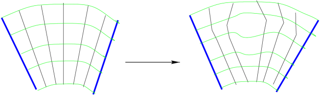
Figure 8: Fluctuations around the minimal helicoid.

Up to now, we restricted ourselves to a classical approximation based on the evaluation of minimal surfaces solutions for the various Wilson loops involved in the preceeding calculations. It is interesting to note [7] that a further step can be done by evaluating the contribution of quadratic fluctuations of the string worldsheet around the minimal surfaces in the case where these surfaces are embedded in helicoids, as discussed for the confining backgrounds. The semi classical correction comes from the fluctuations near the minimal surface sketched in Fig.8. The main outcome is that this semi classical correction can be computed and is intimately related to the well-known “universal” Lüscher term contribution to the interquark potential [23].

The fluctuation determinant for the case of a helicoid bounded by two helices with $\tau=\pm{\cal T}$ has already been calculated [6, 7]. Let us briefly recall the basic steps. First one reparametrizes the helicoid by replacing the variable $\tau$ in (10) by

$$\rho=\frac{L}{\theta}\ \log\left(\frac{\theta\tau}{L}+\sqrt{1+\frac{\theta^{2}\tau^{2}}{L^{2}}}\right)\ .$$ (34)

In the variables $\rho$, $\sigma$ the induced metric on the helicoid has a conformal factor i.e.

$$g_{ab}=(\cosh^{2}\theta\rho/L)\ \ \delta_{ab}\ .$$ (35)

Therefore, since string theory in the AdS background is expected to be critical (conformal invariant), we may perform the calculation getting rid of the conformal factor, i.e. for the conformally equivalent flat metric $g_{ab}=\delta_{ab}$. This reduces to a calculation of the fluctuation determinant for a rectangle of size $a\times b$ where

$$a=L\ ;\ b=\frac{2L}{\theta}\log\left(\theta{\cal T}/L+\sqrt{1+\theta^{2}{\cal T}^{2}/L^{2}}\right)\ .$$ (36)

Furthermore, we assume that the quadratic bosonic fluctuations are governed by the Polyakov action, as is indeed the case for string theories on AdS backgrounds. For high energies (after continuation to Minkowski space at large $a/b={\cal O}(\log s)\gg 1$) one obtains

$$Fluct.(\tau(\sigma)\equiv{\cal T})\to\exp\left(\frac{n_{\perp}\cdot\pi}{24}\cdot\frac{a}{b}\right)\ ,$$ (37)

where $n_{\perp}$ is the number of zero modes in the transverse-to-the-branes directions. The result is just equivalent to the Lüscher term in the potential (c.f. Ref.[23]) except that the number of zero modes $n_{\perp}=D-2$ can be larger than the usual value (2) corresponding to flat $4D$ space.

Let us consider the resulting amplitudes after account taken of the fluctuation contributions:

For elastic dipole-dipole scattering, see the discussion in subsection 3.2, one considers [6, 7] the analytic continuation of the minimal area when $\theta\to\chi/\pi.$ Retaining here also the dominant term in the $b\to\frac{4i\pi L}{\chi}$ for large $\chi\sim\log s,$ one obtains the fluctuation-corrected “Pomeron” amplitude

$$A_{\cal P}(s,t)\propto s^{\alpha_{\cal P}(t)}=s^{1+\frac{n_{\perp}}{96}+\frac{\alpha_{eff}^{\prime}}{4}t}\ .$$ (38)

For two-body inelastic scattering, see the discussion in subsection 3.3, one has to implement the minimal condition (31) namely $b\equiv\frac{i\pi L}{\chi}.$ Hence, the fluctuation-corrected “Reggeon” trajectory (cf. 33) reads:

$$A_{\cal R}(s,t)\propto s^{\alpha_{\cal R}(t)}\ =s^{\frac{n_{\perp}}{24}+{\alpha_{eff}^{\prime}}t}\ .$$ (39)

Let us comment these results. The first observation is that in both cases, the slope is determined by minimal surface solutions through the logarithmic contribution in the helicoid area. The factor four in the slope comes from the specific saddle point path integral over the exchanged quark trajectories (for Reggeon exchange). It is interesting to note that this theoretical feature is in qualitative agreement with the phenomenology of soft scattering. Indeed once we fix the $\alpha_{eff}^{\prime}$ from the phenomenological value of the static $q\bar{q}$ potential ($\alpha_{eff}^{\prime}\sim 0.9\,GeV^{-2}$) we get for the slopes $\alpha_{R}=\alpha_{eff}^{\prime}\sim 0.9\,GeV^{-2}$ and $\alpha_{P}=\alpha_{eff}^{\prime}/4\sim 0.23\,GeV^{-2}$ in good agreement with the phenomenological slopes.

The second feature is the relation between the Pomeron and Reggeon intercepts. At the classical level of our approach these are respectively 1 and 0. Note that this classical piece is in agreement with what is obtained from simple exchanges of two gluons and quark-antiquark pair, respectively, in the $t$ channel. The fluctuation (quantum) contributions to the Reggeon and Pomeron are also related by the factor four.

Adding both classical and fluctuation contributions gives an estimate which is in qualitative agreement with the observed intercepts. Indeed, when calculating the fluctuations around a minimal surface near the horizon in the BH backgrounds there could be $n_{\perp}=7,8$ massless bosonic modes [12]. For $n_{\perp}=7,8$ one gets $1.073-1.083$ for the Pomeron and $0.3-0.33$ for the Reggeon. This result is in agreement with the observed intercept for the “Pomeron” and somewhat below the intercepts of around $0.5$ observed for the dominant Reggeon trajectories.

An interesting feature of the results is the key role of the logarithmic term in the formulae (cf. (11) for the area of the truncated helicoids. Besides the main feature being that it leads, through its analytical structure, to Reggeization, it also gives rise to the possibility of additional contributions from crossing different Riemann sheets ($log\to log+2\pi ik$) in the course of performing analytical continuation from Euclidean to Minkowski space .

For instance in the “Reggeon” case, the amplitude in impact parameter space (33) picks up new multiplicative factors:

$$e^{-\frac{L^{2}}{4\alpha_{eff}^{\prime}\log s}}\cdot e^{-k\frac{L^{2}}{\alpha_{eff}^{\prime}\log s}}\ .$$ (40)

This can be interpreted (for $k>0$) as $k$-Pomeron exchange corrections to a single Reggeon exchange. Indeed the slope of the trajectory obtained from Fourier transform of formula (40) is the one expected from such contributions.

5 Conclusion: Reggeization and confinement

The interesting output of the application of AdS/CFT correspondence to high energy amplitudes at strong coupling is to emphasize the relation between Reggeization and confinement, using the description of two-body scattering amplitudes in the dual string theory. Lattice calculations, which is the only presently known way to evaluate directly QCD observables at strong coupling, are not able to compute high-energy amplitudes.

When comparing AdS₅ duality - which corresponds to a conformal, non-confining gauge theory - with AdS_BH duality, which leads to reggeization, the difference ultimately comes from the different metrics in the bulk and thus from the different geometrical features of the minimal surfaces for the same boudary conditions. In particular, taking into account their different geometry, see e.g. Fig.9, one expects after analytic continuation and in the large energy ($\chi\to\infty$) limit:

$$Area^{AdS}_{min}\sim\lim_{\chi\to\infty}\frac{L}{L/\chi}\ ;\ Area^{BH}_{min}\sim\lim_{\chi\to\infty}L\times\frac{L}{\chi}\ .$$ (41)

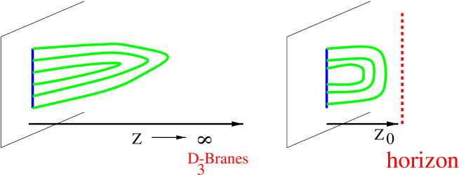
Figure 9: Comparison of $AdS_{5}$ and $AdS_{BH}$ minimal contours at high energy.

The AdS₅ case leads to a $L$-invariant value, as it is scale invariant, and, after Fourier transformation, to a high-energy amplitude with a $q^{2}$ independent energy exponent (or flat Regge trajectory), see formula (14). On the other hand, the AdS_BH case leads to a linear Regge trajectory after Fourier transformation. For the AdS_BH case this rough expectation can be verified by an explicit calculation. Hence confinement appears as an essential ingredient for the reggeized structure of two-body high-energy amplitudes. We expect this result not to be dependent on the precise geometrical AdS_BH setting and thus to indicate a quite general property of confining theories.

As a conclusion, let us summarize our results:

• The AdS/CFT correspondence can be used to give a geometrical formulation of two-body scattering amplitudes in the gravitational dual of gauge field theories.

• The consideration of quark-quark scattering in physical Minkowski space shows that the main geometrical features of two-body scattering amplitudes are related to a (generalized to AdS metrics) helicoidal structure of minimal surfaces in Euclidian space via analytical continuation.

• In the case of non conformal theories, such as the $AdS_{BH}$ case, the metrics is approximately flat near the horizon corresponding to the confinement scale. The (flat space) helicoidal solutions lead to amplitudes with linear Regge slopes.

• While quark-quark scattering is entailed by a cut-off dependence, colourless dipole scattering give rise to cut-off free amplitudes. In particular the two-body dipole-dipole scattering with quark exchange leads to unambiguous results with well-defined regge behaviour.

• Regge trajectories come out linear, with slopes and intercepts related to the quark potential. They include a semi-classical correction due to the fluctuation around the minmal surfaces which are similar to a Lüscher term, but in a 10-dimensional string framework.

• The Pomeron (elastic case) intercept is $1+\epsilon$ where $\epsilon$ is related to a Lüsher term. There exists a factor four between the Reggeon (inelastic case) and Pomeron Regge slopes in agreement with “soft scattering” phenomenology.

In conclusion, the AdS/CFT framework give new insights on the 35-years-old puzzle of high-energy amplitudes at strong gauge coupling.

As a short outlook let us list some interesting problems for future work:

• High-energy phenomenology: Many aspects, like the Flavor/Spin dependences, remain to be studied.

• Approximations: The dual gauge theory is not specified, and the exact minimal surface in the bulk metrics to be determined.

• Dual of QCD? In the present framework, the confining scale $R_{0}$ has no relation with $\Lambda_{QCD}.$

• Unitarity: A more complete investigation requires the study of multi-leg amplitudes.

• Deeper general problems: The formulation of string theory in AdS backgrounds and last but not least, a proof of the AdS/CFT conjecture.

- [1] For a good introduction to String theory models and problems for strong interactions, see P.H.Frampton, Dual Resonance Models , (1974, Benjamin; New edition: 1986, World Scientific).
- [2] A.M. Polyakov, Nucl.Phys.Proc.Suppl. 68 (1998) 1.
- [3] J. Polchinski and M.J. Strassler, Phys. Rev. Lett. 88 (2002) 031601.
- [4] R.A. Janik and R. Peschanski, Nucl. Phys. B565 (2000) 193.
- [5] R.A. Janik and R. Peschanski, Nucl. Phys. B586 (2000) 163.
- [6] R.A. Janik and R. Peschanski, Nucl. Phys. B625 (2002) 279.
- [7] R.A. Janik, Phys. Lett. B500 (2001) 118.
- [8] J. Maldacena, Adv. Theor. Math. Phys. 2 (1998) 231; S.S. Gubser, I.R. Klebanov and A.M. Polyakov, Phys. Lett. B428 (1998) 105.
- [9] For a detailed review and an extensive list of references, please refer to: O. Aharony, S.S. Gubser, J. Maldacena, H. Ooguri and Y. Oz, Phys.Rept. 323 (2000)183.
- [10] E. Witten, Adv. Theor. Math. Phys. 2 (1998) 505.
- [11] H. Ooguri, H. Robins and J. Tannenhauser, Phys. Lett. B437 (1998) 77.
- [12] Y. Kinar, E. Schreiber, J. Sonnenschein and N. Weiss, Nucl. Phys. B583 (2000) 76.
- [13] A. Kehigas and K. Sfetsos, Phys. Lett. B456 (1999) 22.
- [14] C. Angelantonj and A. Armoni, Phys. Lett. B482 (2000) 329.
- [15] J. Maldacena, Phys. Rev. Lett. 80 (1998) 4859; S.-J. Rey and J. Yee, hep-th/9803001; JJ. Sonnenschein and A. Loewy, JHEP 0001 (2000) 042.
- [16] M. Rho, S.-J. Sin and I. Zahed, Phys. Lett. B466 (1999) 199.
- [17] N. Drukker, D.J. Gross and H. Ooguri, Phys.Rev., D60 (1999) 125006;H. Ooguri, Prog.Theor.Phys.Suppl., 134 (1999) 153.
- [18] L.N. Lipatov, Sov. J. Nucl. Phys. 23 (1976) 642; V.S. Fadin, E.A. Kuraev and L.N. Lipatov, Phys. Lett. B60 (1975) 50; E.A. Kuraev, L.N. Lipatov and V.S. Fadin, Sov. Phys. JETP 44 (1976) 45, 45 (1977) 199; I.I. Balitsky and L.N. Lipatov, Sov. J. Nucl. Phys. 28 (1978) 822.
- [19] O. Nachtmann, High Energy Collisions and Nonperturbative QCD, Lectures given at Banz (Germany) 1993 and at Schladming (Austria) 1996, hep-ph/9609365.
- [20] E. Meggiolaro, Z. Phys. C76 (1997) 523; , Nucl. Phys. B625 (2002) 312.
- [21] J.C.C. Nitsche, Lectures on minimal surfaces, Cambridge University Press,1989.
- [22] R.P. Feynman, Phys. Rev. 80 (1950) 440 A. M. Polyakov, Mod. Phys. Lett. A3 (1988) 325. G. P. Korchemsky, Int. J. Mod. Phys. A7 (1992) 339; , Phys. Lett. B232 (1989) 334.
- [23] M. Lüscher, K. Symanzik and P. Weisz, Nucl.Phys. B173 (1980) 365. O. Alvarez, Phys.Rev. D24 (1981) 440.