Status of Evidence for
Neutrinoless Double Beta Decay

Abstract

The present experimental status in the search for neutrinoless double beta decay is reviewed, with emphasis on the first indication for neutrinoless double beta decay found in the HEIDELBERG-MOSCOW experiment, giving first evidence for lepton number violation and a Majorana nature of the neutrinos. Future perspectives of the field are briefly outlined.

1 Introduction

The neutrino oscillation interpretation of the atmospheric and solar neutrino data, deliver a strong indication for a non-vanishing neutrino mass. While such kind of experiments yields information on the difference of squared neutrino mass eigenvalues and on mixing angles (for the present status see, e.g. Bahc01 ; Barg02-Sol ), the absolute scale of the neutrino mass is still unknown. Information from double beta decay experiments is indispensable to solve these questions KKPS1-2 ; KK60Y . Another important problem is that of the fundamental character of the neutrino, whether it is a Dirac or a Majorana particle Majorana37 ; Rac37 . Neutrinoless double beta decay could answer also this question. Perhaps the main question, which can be investigated by double beta decay with high sensitivity, is that of lepton number conservation or non-conservation.

Double beta decay, the rarest known nuclear decay process, can occur in different modes:

$2\nu\beta\beta-\rm decay:$	$A(Z,N)\rightarrow A(Z\!+\!2,N\!-\!2)+2e^{-}+2\bar{\nu}_{e}$          (1)
$0\nu\beta\beta-\rm decay:$	$A(Z,N)\rightarrow A(Z\!+\!2,N\!-\!2)+2e^{-}$                  (2)
$0\nu(2)\chi\beta\beta-\rm decay:$	$A(Z,N)\rightarrow A(Z\!+\!2,N\!-\!2)+2e^{-}+(2)\chi$         (3)

While the two-neutrino mode (1) is allowed by the Standard Model of particle physics, the neutrinoless mode ($0\nu\beta\beta$ ) (2) requires violation of lepton number ($\Delta$L=2). This mode is possible only, if the neutrino is a Majorana particle, i.e. the neutrino is its own antiparticle (E. Majorana Majorana37 , G. Racah Rac37 , for subsequent works we refer to Mcl57 ; Case57 ; Ahl96 , for some reviews see Doi85 ; Mut88 ; Gro89/90 ; Kla95/98 ; KK60Y ; Vog2001 ). First calculations of $0\nu\beta\beta$ decay based on the Majorana theory have been done by W.H. Furry Fur39 . The most general Lorentz-invariant parametrization of neutrinoless double beta decay is shown in Fig. 1.

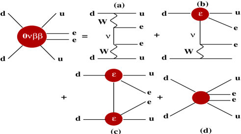
Figure 1: Feynman graphs of the general double beta decay with long range (a-c) and short range (d) parts (see KK-Paes99 ).

The usually used assumption is that the first term (i.e. the Majorana mass mechanism) dominates the decay process. However, as can be seen from Fig. 1, and as discussed elsewhere (see, e.g. KK60Y ; KK-LeptBar98 ; KK-SprTracts00 ; Faes01 ) neutrinoless double beta decay can not only probe a Majorana neutrino mass, but various new physics scenarios beyond the Standard Model, such as R-parity violating supersymmetric models, R-parity conserving SUSY models, leptoquarks, violation of Lorentz-invariance, and compositeness (for a review see KK60Y ; KK-LeptBar98 ; KK-SprTracts00 ). Any theory containing lepton number violating interactions can in principle lead to this process allowing to obtain information on the specific underlying theory. It has been pointed out already in 1982, however, that independently of the mechanism of neutrinoless double decay, the occurence of the latter implies a non-zero neutrino mass and vice versa Sch82a . This theorem has been extended to supersymmetry. It has been shown H_KK_Kov97-98 that if the neutrino has a finite Majorana mass, then the sneutrino necessarily has a (B-L) violating ’Majorana’ mass, too, independent of the mechanism of mass generation. The experimental signature of the neutrinoless mode is a peak at the Q-value of the decay.

Restricting to the Majorana mass mechanism, a measured half-life allows to deduce information on the effective Majorana neutrino mass $\langle m\rangle$ , which is a superposition of neutrino mass eigenstates Doi85 ; Mut88 :

$$[T^{0\nu}_{1/2}(0^{+}_{i}\rightarrow 0^{+}_{f})]^{-1}=C_{mm}\frac{\langle m\rangle^{2}}{m_{e}^{2}}+C_{\eta\eta}\langle\eta\rangle^{2}+C_{\lambda\lambda}\langle\lambda\rangle^{2}+C_{m\eta}\langle\eta\rangle\frac{\langle m\rangle}{m_{e}}$$ (1)

$$+C_{m\lambda}\langle\lambda\rangle\frac{\langle m_{\nu}\rangle}{m_{e}}+C_{\eta\lambda}\langle\eta\rangle\langle\lambda\rangle,$$ (2)

$${}\langle m\rangle=|m^{(1)}_{ee}|+e^{i\phi_{2}}|m_{ee}^{(2)}|+e^{i\phi_{3}}|m_{ee}^{(3)}|~{},$$ (3)

where $m_{ee}^{(i)}\equiv|m_{ee}^{(i)}|\exp{(i\phi_{i})}$ ($i=1,2,3$) are the contributions to $\langle m\rangle$ from individual mass eigenstates, with $\phi_{i}$ denoting relative Majorana phases connected with CP violation, and $C_{mm},C_{\eta\eta},...$ denote nuclear matrix elements squared, which can be calculated, (see, e.g. Sta90 , for a review and some recent discussions see e.g. Tom91 ; KK60Y ; Mut88 ; Gro89/90 ; FaesSimc ; St-KK01-1 ; St-KK01-2 ; Faes01 ). Ignoring contributions from right-handed weak currents on the right-hand side of eq.(1), only the first term remains.

The effective mass is closely related to the parameters of neutrino oscillation experiments, as can be seen from the following expressions

$${}|m^{(1)}_{ee}| = |U_{e1}|^{2}m_{1},$$ (4)

$$|m^{(2)}_{ee}| = |U_{e2}|^{2}\sqrt{\Delta m^{2}_{21}+m_{1}^{2}},$$ (5)

$$|m^{(3)}_{ee}| = |U_{e3}|^{2}\sqrt{\Delta m^{2}_{32}+\Delta m^{2}_{21}+m_{1}^{2}},$$ (6)

Here, $U_{ei}$ are entries of the neutrino mixing matrix, and $\Delta m^{2}_{ij}~{}=~{}|m^{2}_{i}-m^{2}_{j}|$, with $m_{i}$ denoting neutrino mass eigenstates. $U_{ei}$ and $\Delta m^{2}$ can be determined from neutrino oscillation experiments.

The importance of $\langle m\rangle$ for solving the problem of the structure of the neutrino mixing matrix and in particular to fix the absolute scale of the neutrino mass spectrum which cannot be fixed by $\nu$ - oscillation experiments alone, has been discussed in detail in e.g. KK-Sar_Evid01 ; KKPS1-2 ; Viss01 .

Double beta experiments to date gave only upper limits for the effective mass. The most sensitive limits HM97a ; HM99 ; HDM01 were already of striking importance for neutrino physics, excluding for example, in hot dark matter models, the small mixing angle (SMA) MSW solution of the solar neutrino problem Gla00 ; Ellis99 ; Adh99 ; Minak-Nuno ; Minak01 ; Minak97 ; KKPS1-2 ; KK60Y in degenerate neutrino mass scenarios.

The HEIDELBERG-MOSCOW double beta decay experiment in the Gran Sasso Underground Laboratory KK-Prop87 ; KK-Neutr98 ; Kla96b ; KK-LeptBar98 ; KK-StProc00 ; KK60Y searches for double beta decay of ${}^{76}{Ge}\longrightarrow^{76}{Se}$ + 2 $e^{-}$ + (2$\bar{\nu}$) since 1990. It is the most sensitive double beta experiment since almost eight years now. The experiment operates five enriched (to 86$\%$) high-purity ${}^{76}{Ge}$ detectors, with a total mass of 11.5 kg, the active mass of 10.96 kg being equivalent to a source strength of 125.5 mol ${}^{76}{Ge}$ nuclei.

In this paper, we present a new, refined analysis of the data obtained in the HEIDELBERG-MOSCOW experiment during the period August 1990 - May 2000 which have recently been published HDM01 . The analysis concentrates on the neutrinoless decay mode which is the one relevant for particle physics (see, e.g. KK60Y ). First evidence for the neutrinoless decay mode will be presented (a short communication has been given already in KK-Evid01 (see also KK-China01 ), and first reactions have been published already KK-Sar_Evid01 ; KK3-Sar_Evid01 ; Ma02-Ev ; Barg02-Ev ; Ueh02-Ev ; Min-Evid02 ; Chat-Evid02 ; Xing-Evid02 ; Ham-Evid02 ; Ahl-Kirch-Evid02 ; Nature02-Evid ; Ma-Evid2-02 ; Hab-Suz02 ; Mohap02-Evid ; Kays02-Evid ; Fodor02-Evid ; Pakv02-Evid ; Niels02 ; He02-Evid ; Josh02-Evid ; Bran02-Evid ; Cheng02-Evid ; Smirn02-Evid ; Mats02-Evid ; Wiss-Evid02 ). For the results concerning 2$\nu\beta\beta$ decay and Majoron-accompanied decay we refer to HDM01 . The results will be put into the context of other present $\beta\beta$ activities.

2 Experimental Set-up and Results

A detailed description of the HEIDELBERG-MOSCOW experiment has been given recently in HDM97 , and in HDM01 . Therefore only some important features will be given here. We start with some general notes.

1. Since the sensitivity for the $0\nu\beta\beta$ half-life is

$${}T^{0\nu}_{1/2}\sim a\times\epsilon\sqrt{\frac{Mt}{\Delta EB}}$$ (7)

(and $\frac{1}{\sqrt{T^{0\nu}}}\sim\langle m_{\nu}\rangle$), with a denoting the degree of enrichment, $\epsilon$ the efficiency of the detector for detection of a double beta event, M the detector (source) mass, $\Delta E$ the energy resolution, B the background and t the measuring time, the sensitivity of our 11 kg of enriched ${}^{76}{Ge}$ experiment corresponds to that of an at last 1.2 ton natural Ge experiment. After enrichment, energy resolution, background and source strength are the most important features of a $\beta\beta$ experiment.

2. The high energy resolution of the Ge detectors of 0.2$\%$ or better, assures that there is no background for a $0\nu\beta\beta$ line from the two-neutrino double beta decay in this experiment, in contrast to most other present experimental approaches, where limited energy resolution is a severe drawback.

3. The efficiency of Ge detectors for detection of $0\nu\beta\beta$ decay events is close to 100 $\%$ (95%, see Diss-Dipl ).

4. The source strength in this experiment of 11 kg is the largest source strength ever operated in a double beta decay experiment.

5. The background reached in this experiment is, with 0.17 events/kg y keV in the $0\nu\beta\beta$ decay region (around 2000-2080 keV), the lowest limit ever obtained in such type of experiment.

6. The statistics collected in this experiment during 10 years of stable running is the largest ever collected in a double beta decay experiment.

7. The Q value for neutrinoless double beta decay has been determined recently with very high precision to be Q_ββ=2039.006(50) keV New-Q-2001 ; Old-Q-val .

	Total	Active	Enrichment	FWHM 1996	FWHM 2000
Detector	Mass	Mass	in ${}^{76}{Ge}$	at 1332 keV	at 1332 keV
Number	[kg]	[kg]	[$\%$]	[keV]	[keV]
No. 1	0.980	0.920	85.9 $\pm$ 1.3	2.22 $\pm$ 0.02	2.42 $\pm$ 0.22
No. 2	2.906	2.758	86.6 $\pm$ 2.5	2.43 $\pm$ 0.03	3.10 $\pm$ 0.14
No. 3	2.446	2.324	88.3 $\pm$ 2.6	2.71 $\pm$ 0.03	2.51 $\pm$ 0.16
No. 4	2.400	2.295	86.3 $\pm$ 1.3	2.14 $\pm$ 0.04	3.49 $\pm$ 0.24
No. 5	2.781	2.666	85.6 $\pm$ 1.3	2.55 $\pm$ 0.05	2.45 $\pm$ 0.11

Table 1: Technical parameters of the five enriched detectors. (FWHM - full width at half maximum.)

We give now some experimental details. All detectors (whose technical parameters are given in Table 1 (see HDM97 )), except detector No. 4, are operated in a common Pb shielding of 30 cm, which consists of an inner shielding of 10 cm radiopure LC2-grade Pb followed by 20 cm of Boliden Pb. The whole setup is placed in an air-tight steel box and flushed with radiopure nitrogen in order to suppress the ${}^{222}{Rn}$ contamination of the air. The steel box is centered inside a 10-cm boron-loaded polyethylene shielding to decrease the neutron flux from outside. An active anticoincidence shielding is placed on the top of the setup to reduce the effect of muons. Detector No. 4 is installed in a separate setup, which has an inner shielding of 27.5 cm electrolytical Cu, 20 cm lead, and boron-loaded polyethylene shielding below the steel box, but no muon shielding. Fig. 2 gives a view of the experimental setup.

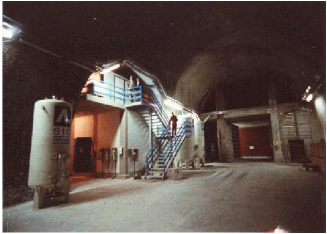
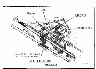
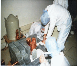
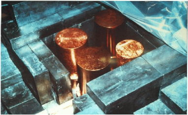
Figure 2: The $\beta\beta$-laboratory of the HEIDELBERG-MOSCOW experiment in the Gran Sasso (upper left) and its location between halls A and B (upper right), and four of the enriched detectors during installation (lower part).

To check the stability of the experiment, a calibration with a ${}^{228}{Th}$ and a ${}^{152}{Eu}$+${}^{228}{Th}$, and a ${}^{60}{Co}$ source is done weekly. High voltage of the detectors, temperature in the detector cave and the computer room, the nitrogen flow in the detector boxes, the muon anticoincidence signal, leakage current of the detectors, overall and individual trigger rates are monitored daily. The energy spectrum is taken in 8192 channels in the range from threshold up to about 3 MeV, and in a parallel spectrum up to about 8 MeV.

Because of the big peak-to-Compton ratio of the large detectors, external $\gamma$ activities are relatively easily identified, since their Compton continuum is to a large extent shifted into the peaks. The background identified by the measured $\gamma$ lines in the background spectrum consists of:

1. primordial activities of the natural decay chains from ${}^{238}{U}$, ${}^{232}{Th}$, and ${}^{40}{K}$

2. anthropogenic radio nuclides, like ${}^{137}{Cs}$, ${}^{134}{Cs}$, ${}^{125}{Sb}$, ${}^{207}{Bi}$

3. cosmogenic isotopes, produced by activation due to cosmic rays.

   The activity of these sources in the setup is measured directly and can be located due to the measured and simulated relative peak intensities of these nuclei.

   Hidden in the continuous background are the contributions of

4. the bremsstrahlungs spectrum of ${}^{210}{Bi}$ (daughter of ${}^{210}{Pb}$),

5. elastic and inelastic neutron scattering, and

6. direct muon-induced events.

External $\alpha$ and $\beta$ activities are shielded by the 0.7-mm inactive zone of the p-type Ge detectors on the outer layer of the crystal. The enormous radiopurity of HP-germanium is proven by the fact that the detectors No. 1, No. 2 and No. 3 show no indication of any $\alpha$ peaks in the measured data. Therefore no contribution of the natural decay chains can be located inside the crystals. Detectors No. 4 and No. 5 seem to be slightly contaminated with ${}^{210}{Pb}$ on the level of few $\mu$Bq/kg, most likely surface contaminations at the inner contact. This contamination was identified by a measured $\alpha$ peak in the background spectrum at 5.305 MeV of the daughter ${}^{210}{Po}$ and the constant time development of the peak counting rate. There is no contribution to the background in the interesting evaluation areas of the experiment due to this activity. For further details about the experiment and background we refer to HDM97 ; Diss-Dipl (see also Table 2).

In the vicinity of the Q-value of the double beta decay of Q_ββ = 2039.006(50)  keV, very weak lines at 2034.744 and 2042 keV from the cosmogenic nuclide ${}^{56}{Co}$, and from ${}^{214}{Bi}$ (${}^{238}U$-decay chain) at 2010.7, 2016.7, 2021.8 and 2052.9 keV, may be expected.

On the other hand, there are no background $\gamma$-lines at the position of an expected $0\nu\beta\beta$ line, according to our Monte Carlo analysis of radioactive impurities in the experimental setup Diss-Dipl and according to the compilations in Tabl-Isot96 .

In total 55 possible $\gamma$-lines from various isotopes in the region between 2037 and 2041 keV are known Tabl-Isot96 . Only 5 of the isotopes responsible for them ($\rm{}^{102}Rh$, $\rm{}^{146}Eu$, $\rm{}^{124}I$, $\rm{}^{124}Sb$ and $\rm{}^{170}Lu$) have half-lifes larger than 1 day. However, some of the isotopes yielding lines in this energy range can in principle be produced by inelastic hadron reactions (induced by muons or neutrons).

Therefore each of these 55 isotopes was checked for the existence of a $\gamma$-line from the isotope which has a high emission probability $I_{h}$. A search was made for this $\gamma$-line in the measured spectrum to obtain its intensity ($S_{h}$) or an upper limit for it. Then the adopted intensity $S_{0}$ for a $\gamma$-line from the same isotope in the area around $\sim$2039 keV can be calculated by using the emission probability $I_{0}$ for the line at $\sim$2039 keV. Different absorption for gammas of different energies are taken into account in a schematic way.

Detec-	Life	Date	Shielding			Background${{}^{*})}$	PSA
						[counts/
tor	Time					keV y kg]
					boron-	2000.-2100.
Number	[ days ]	Start End	Cu	Pb	poly.	keV
No.1	387.6	8/90-8/91	yes			A0.56	Ano
		1/92-8/92					Ano
No.2	225.4	9/91 - 8/92		yes		A0.29	Ano
Common shielding for three detectors
No.1	382.8	9/92 - 1/94		yes		A0.22	Ano
No.2	383.8	9/92 - 1/94		yes		A0.22	Ano
No.3	382.8	9/92 - 1/94		yes		A0.21	Ano
No.1	263.0	2/94 - 11/94		yes	yes	A0.20	Ano
No.2	257.2	2/94 - 11/94		yes	yes	A0.14	Ano
No.3	263.0	2/94 - 11/94		yes	yes	A0.18	Ano
Full Setup
Four detectors in common shielding, one detector separate
No.1	203.6	12/94 - 8/95		yes	yes	A0.14	Ano
No.2	203.6	12/94 - 8/95		yes	yes	A0.17	Ano
No.3	188.9	12/94 - 8/95		yes	yes	A0.20	Ano
No.5	48.0	12/94 - 8/95		yes	yes	A0.23	since 2/95
No.4	147.6	1/95 - 8/95	yes			A0.43	Ano
No.1	203.6	11/95 - 05/00		yes	yes	A0.170	Ano
No.2	203.6	11/95 - 05/00		yes	yes	A0.122	Ayes
No.3	188.9	11/95 - 05/00		yes	yes	A0.152	Ayes
No.5	48.0	11/95 - 05/00		yes	yes	A0.159	Ayes
No.4	147.6	11/95 - 05/00	yes			A0.188	Ayes

Table 2: Development of the experimental set-up and of the background numbers in the different data acquisition periods for the enriched detectors of the HEIDELBERG-MOSCOW experiment. ${{}^{*})}$ Without PSA method.

If the calculated intensity $S_{l}<1$ for the $\gamma$-line in the interesting area, this isotope can be safely excluded to contribute a significant part to the background.

For example, the isotope $\rm{}^{139}Xe$ possesses a $\gamma$-line at 2039.1 keV with an emission probability of 0.078%. This isotope also possesses a $\gamma$-line at 225.4 keV with an emission probability of 3.2%. The intensity of the line at 225.4 keV in our spectrum was measured to be $<$6.5 counts. This means that the $\gamma$-line at 2039.1 keV has $<2\frac{0.078}{3.2}6.5=0.32$ counts, and therefore can be excluded.

Only eight isotopes could contribute a few counts according to the calculated limits, in the interesting area for the $0\nu\beta\beta$ -decay area: $\rm{}^{52m}Fe$, $\rm{}^{93m}Ru$, $\rm{}^{120}In$, $\rm{}^{131}Ce$, $\rm{}^{170}Lu$, $\rm{}^{170m}Ho$, $\rm{}^{174}Ta$ and $\rm{}^{198}Tl$. Most of them have a half-life of a few seconds, only $\rm{}^{170}Lu$ has a half-life of 2.01 days, and no one of them has a longer living mother isotope. To contribute to the background they must be produced with a constant rate, e.g. by inelastic neutron and/or muon reactions. Only 5 isotopes can be produced in a reasonable way, by the reactions listed in Tabl. 3.

isotope	$\rm{}^{52m}Fe$	$\rm{}^{93m}Ru$	$\rm{}^{120}In$	$\rm{}^{170m}Ho$	$\rm{}^{198}Tl$
production	$\rm{}^{50}Cr$($\alpha,2n\gamma$)	$\rm{}^{92}Mo$($\alpha,3n$)	$\rm{}^{120}Sn$($n,p$),	$\rm{}^{170}Er$($n,p$)	$\rm{}^{197}Au$($\alpha,3n\gamma$)
reaction			$\rm{}^{123}Sb$($n,\alpha$)

Table 3: Possible reactions (second line) which could produce the isotopes listed in the first line (see toi ).

Except $\rm{}^{120}Sb$ each of the target nuclides is stable. All reactions induced with $\alpha$-particles can be excluded due to the very short interaction length of $\alpha$-particles. Two possibilities remaining to explain possible events in the $0\nu\beta\beta$ -decay area would be:

• $\rm{}^{120}Sn$($n,p$)$\rm{}^{120}In$:
  The cross section for this reaction is 2.5$\pm$1 mb for $E_{n}=14.5$ MeV ref1 . Assuming a neutron flux of (0.4$\pm$0.4)$\times 10^{-9}\frac{1}{cm^{2}\;s}$ for neutrons with an energy between 10-15 MeV as measured in the Gran Sasso Arn99 the rate of $\rm{}^{120}In$ atoms produced per year is about $2\times 10^{-5}$ when there are 50 g of $\rm{}^{120}Sn$ in the detector setup. Even when the cross-section is larger for lower energies, this can not contribute a significant number of counts to the background.

• $\rm{}^{170}Er$($n,p$)$\rm{}^{170m}Ho$:
  The cross section for this reaction is about 1.13$\pm$1 mb for $E_{n}=14.8$ MeV ref2 . Assuming again a neutron flux of (0.4$\pm$0.4)$\times 10^{-9}\frac{1}{cm^{2}\;s}$ for neutrons with an energy between 10-15 MeV the rate of $\rm{}^{170}Er$ atoms produced per year is even less when assuming 50 g of $\rm{}^{120}Er$ in the detector-setup.

In both cases it would be not understandable, how such large amounts of $\rm{}^{120}Sn$ or $\rm{}^{170}Er$ could have come into the experimental setup. Concluding we do not find indications for any nuclides, that might produce $\gamma$-lines with an energy around 2039 keV in the experimental setup.

Fig. 3 shows the combined spectrum of the five enriched detectors obtained over the period August 1990 - May 2000, with a statistical significance of 54.981 kg y (723.44 molyears). (Note that in Fig. 1 of HDM01 ) only the spectrum of the first detector is shown, but normalized to 47.4 kg y Errat-ZPh01 ). The identified background lines give an indication of the stability of the electronics over a decade of measurements. The average rate (sum of all detectors) observed over the measuring time, has proven to be constant within statistical variations. Fig. 5 shows the part of the spectrum shown in Fig. 3, in more detail around the Q-value of double beta decay. Fig. 5 shows the spectrum of single site events (SSE) obtained for detectors 2,3,5 in the period November 1995 - May 2000, under the restriction that the signal simultaneously fulfills the criteria of all three methods of pulse shape analysis we have recently developed HelKK00 ; KKMaj99 and with which we operate all detectors except detector 1 (significance 28.053 kg y) since 1995.

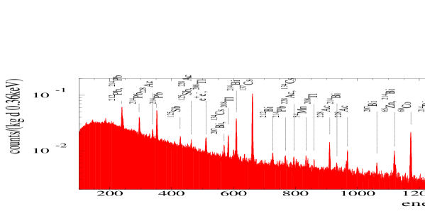
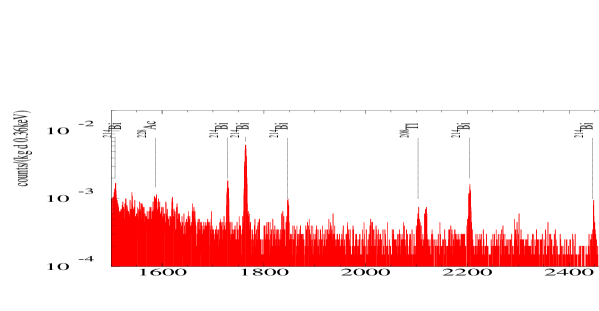
Figure 3: Sum spectrum of enriched detectors Nr. 1,2,3,4,5 over the period August 1990 - May 2000 (54.9813 kg y) measured in the HEIDELBERG-MOSCOW experiment (binning 0.36 keV). The sources of the main identified background lines are noted.

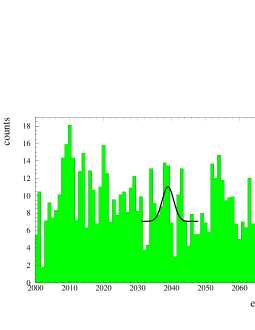
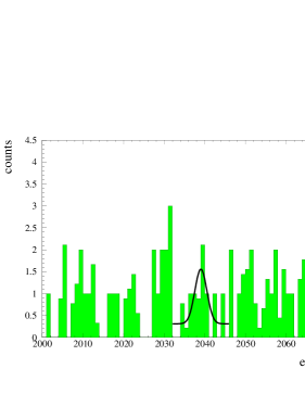
Figure 4: Sum spectrum of the ${}^{76}{Ge}$ detectors Nr. 1,2,3,4,5 over the period August 1990 to May 2000, (54.9813 kg y) in the energy interval 2000 - 2080 keV, around the Q_ββ value of double beta decay (Q_ββ = 2039.006(50) keV) summed to 1 keV bins. The curve results from Bayesian inference in the way explained in sec.3. It corresponds to a half-life T${}_{1/2}^{0\nu}$=(0.80 - 35.07)$\times~{}10^{25}$ y (95% c.l.)

Figure 5: Sum spectrum of single site events, measured with the detectors Nr. 2,3,5 operated with pulse shape analysis in the period November 1995 to May 2000 (28.053 kg y), summed to 1 keV bins. Only events identified as single site events (SSE) by all three pulse shape analysis methods HelKK00 ; Patent-KKHel ; KKMaj99 have been accepted. The curve results from Bayesian inference in the way explained in sec.3. When corrected for the efficiency of SSE identification (see text), this leads to the following value for the half-life: T${}_{1/2}^{0\nu}$=(0.88 - 22.38)$\times~{}10^{25}$ y (90% c.l.).

Double beta events are single site events confined to a few mm region in the detector corresponding to the track length of the emitted electrons. In all three methods, mentioned above, the output of the charge-sensitive preamplifiers was differentiated with 10-20 ns sampled with 250 MHz and analysed off-line. The methods differ in the analysis of the measured pulse shapes. The first one relies on the broadness of the charge pulse maximum, the second and third one are based on neural networks. All three methods are ’calibrated’ with known double escape (mainly SSE) and total absorption (mainly MSE) $\gamma$-lines HelKK00 ; Patent-KKHel ; KKMaj99 ; Diss-Dipl . They allow to achieve about 80$\%$ detection efficiency for both interaction types.

The expectation for a $0\nu\beta\beta$ signal would be a line of single site events on some background of multiple site events but also single site events, the latter coming to a large extent from the continuum of the 2614 keV $\gamma$-line from ${}^{208}{Tl}$ (see, e.g., the simulation in HelKK00 ). From simulation we expect that about 5$\%$ of the double beta single site events should be seen as MSE. This is caused by bremsstrahlung of the emitted electrons Diss-Dipl .

Installation of PSA has been performed in 1995 for the four large detectors. Detector Nr.5 runs since February 1995, detectors 2,3,4 since November 1995 with PSA. The measuring time with PSA from November 1995 until May 2000 is 36.532 kg years, for detectors 2,3,5 it is 28.053 kg y.

Fig. 6 shows typical SSE and MSE events from our spectrum.

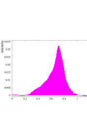
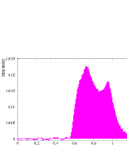
Figure 6: Left: Shape of one candidate for $0\nu\beta\beta$ decay (energy 2038.61 keV) classified as SSE by all three methods of pulse shape discrimination. Right: Shape of one candidate (energy 2038.97 keV) classified as MSE by all three methods.

All the spectra are obtained after rejecting coincidence events between different Ge detectors and events coincident with activation of the muon shield. The spectra, which are taken in bins of 0.36 keV, are shown in Figs. 5,5, Fig.2 of KK-Evid01 in 1 keV bins, which explains the broken number in the ordinate. We do the analysis of the measured spectra with (Fig. 5) and without the data of detector 4 (see Fig.2 in KK-Evid01 , 46.502 kg y) since the latter does not have a muon shield and has the weakest energy resolution. The 0.36 keV bin spectra are used in all analyses described in this work. We ignore for each detector the first 200 days of operation, corresponding to about three half-lives of ${}^{56}{Co}$ ($T_{1/2}$ = 77.27 days), to allow for some decay of short-lived radioactive impurities.

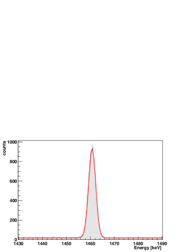
Figure 7: Fit of one the lines (here the 1460.81 keV line from ${}^{40}{K}$) in the sum spectrum of all five detectors, used for the calibration and the determination of the energy resolution (see Table 4).

The background rate in the energy range 2000 - 2080 keV is found to be (0.17 $\pm$ 0.01) events/ kg y keV (without pulse shape analysis) considering all data as background. This is the lowest value ever obtained in such type of experiments. The energy resolution at the Q_ββ value in the sum spectra is extrapolated from the strong lines in the spectrum to be (4.00 $\pm$ 0.39) keV in the spectra with detector 4, and (3.74 $\pm$ 0.42) keV (FWHM) in the spectra without detector 4 (see Fig. 7 and Table 4). The energy calibration of the experiment has an uncertainty of 0.20 keV (see Table 4).

energy [keV]	energy [keV]	width [keV]	width [keV]
fit	from Tabl-Isot96	fit	from calc.
1460.81 $\pm$ 0.02	1460.81	1.49 $\pm$ 0.01	1.49 $\pm$ 0.13
1764.56 $\pm$ 0.05	1764.49	1.70 $\pm$ 0.05	1.59 $\pm$ 0.15
2103.31 $\pm$ 0.45	2103.53	1.86 $\pm$ 0.35	1.71 $\pm$ 0.16
2204.12 $\pm$ 0.14	2204.19	1.89 $\pm$ 0.13	1.74 $\pm$ 0.17
2447.73 $\pm$ 0.26	2447.86	1.82 $\pm$ 0.33	1.82 $\pm$ 0.18
2614.48 $\pm$ 0.07	2614.53	1.80 $\pm$ 0.06	1.88 $\pm$ 0.18

Table 4: Energies and widths of some prominent lines in the sum spectrum of all five detectors determined by our energy calibration and peak fit methods, and comparison with the energy given in the literature Tabl-Isot96 , and the fitted dependence of the width as function of energy.

3 Data Analysis

We analyse the measured spectra with the following methods:

1. Bayesian inference, which is used widely at present in nuclear and astrophysics (see, e.g. Bayes_Method-General ; RPD00 ; Hagan94 ; Dietz-Diss03 ). This method is particularly suited for low counting rates, where the data follow a Poisson distribution, that cannot be approximated by a Gaussian.

2. Feldman-Cousins Method Feldm98 ; RPD00 .

3. Maximum Likelihood Method (see RPD00 ; Kchi-kvadr ).

The Bayesian method is described in the next subsection, 3.1. In subsection 3.2 we give some numerical examples of the sensitivities of this method and of the Maximum Likelihood Method in the search for events of low statistics Dietz-Diss03 .

3.1 The Bayesian Method

We first describe the procedure summarily and then give some mathematical details (see Dietz-Diss03 ).

One knows that the lines in the spectrum are Gaussians with the standard deviation $\sigma$=1.70 keV in Fig. 5 and $\sigma$=1.59 keV in Fig. 5. This corresponds to 4.0(3.7) keV FWHM. Given the position of a line, we used Bayes theorem to infer the contents of the line and the level of a constant background.

Bayesian inference yields the joint probability distribution for both parameters. Since we are interested in the contents of the line, the other parameter was integrated out. This yields the distribution of the line contents. If the distribution has its maximum at zero contents, only an upper limit for the contents can be given and the procedure does not suggest the existence of a line. If the distribution has its maximum at non-zero contents, the existence of a line is suggested and one can define the probability K_E that there is a line with non-zero contents.

We define the Bayesian procedure in some more detail. It starts from the distribution $p(x_{1}...x_{M}|\rho,\eta)$ of the count rates $x_{1}...x_{M}$ in the bins 1..M of the spectrum - given two parameters $\rho,\eta$. The distribution $p$ is the product

$${}p(x_{1}...x_{M}|\rho,\eta)~{}=~{}\prod_{k=1}^{M}\frac{{\lambda_{k}}^{x_{k}}}{x_{k}!}~{}e^{-\lambda_{k}}$$ (8)

of Poissonians for the individual bins. The expectation value $\lambda_{k}$ is the superposition

$${}\lambda_{k}~{}=~{}\rho~{}[\eta~{}f_{1}(k)+(1-\eta)~{}f_{2}(k)]$$ (9)

of the form factors f₁ of the line and f₂ of the background; i.e. f₁(k) is the Gaussian centered at E with the above-mentioned standard deviation value and f₂(k)$\equiv$f₂ is a constant. Note that the model allows for a spectrum of background only, i.e. $\eta$=0, and in this sense also tests the hypothesis ’only background’.

Since

$${}\sum_{k=1}^{M}f_{\nu}(k)~{}=~{}1\hskip 42.67912ptfor~{}~{}\nu=1,2,$$ (10)

one has

$${}\sum_{k=1}^{M}\lambda_{k}~{}=~{}\rho.$$ (11)

Hence, $\rho$ parametrizes the total intensity in the spectrum, and $\eta$ is the relative intensity in the Gaussian line.

The total intensity $\rho$ shall be integrated out. For this purpose, one needs the prior distribution $\mu(\rho|\eta)$ of $\rho$ for fixed $\eta$. We obtain it from Jeffreys’ rule ($\S$5.35 of Hagan94 ).

$${}\mu\,(\rho\,|\,\eta)~{}=~{}{\left|\,\overline{\frac{\partial^{2}}{\partial{\rho}^{2}}\,\ln p}\,\right|}^{1/2}.$$ (12)

The overline denotes the expectation value with respect to $x_{1}...x_{M}$.

The integration

$${}p_{1}\,(x_{1}...x_{M}\,|\,\eta)~{}\sim~{}\int d\rho\,p\,(x_{1}...x_{M}\,|\,\rho,\eta)~{}\mu\,(\,\rho\,|\,\eta)$$ (13)

then yields the model $p_{1}$ conditioned by $\eta$ alone. It is normalized to unity and the prior distribution

$${}\mu_{1}\,(\eta)~{}=~{}{\left|\,\overline{\frac{\partial^{2}}{\partial{\eta}^{2}}\,\ln{p_{1}}}\,\right|}^{1/2}$$ (14)

of $\eta$ is obtained by application of Jeffrey’s rule to $p_{1}$. Bayes’ theorem yields the posterior distribution

$${}P_{1}(\eta|x_{1}...x_{M})~{}=~{}\frac{p_{1}\,(x_{1}...x_{M}\,|\,\eta)\,\mu_{1}(\eta)}{\int d\eta\,p_{1}\,\mu_{1}}$$ (15)

of $\eta$.

From the posterior the ’error interval’ for $\eta$ is obtained. It is the shortest interval in which $\eta$ lies with probability K. The length of an interval is defined by help of the measure $\mu_{1}(\eta)$. We call this the Bayesian interval for the probability K in order to distinguish it from a confidence interval of classical statistics. There is a limit, where Bayesian intervals agree with confidence intervals. See below.

The borders of a Bayesian interval are given by the intersections of the likelihood function $P_{1}\,(\eta\,|\,x)/\mu_{1}(\eta)\sim p_{1}(x|\eta)$ with a horizontal line at $\eta_{l},\,\eta_{h}$ (see Fig. 8). The probability K is obtained by integrating $P_{1}$ from $\eta_{l}$ to $\eta_{h}$.

Figure 8: The figure shows the relation between P₁, K and K_E. K is the integral over P₁ in the limits [$\eta_{l},\eta_{h}$]. The integral over P₁ in the interval [0,$\eta_{E}$] is K_E.

When the likelihood function has its maximum at $\eta=0$, then the Bayesian interval will - for every K - include $\eta=0$. Then this value cannot be excluded and only an upper limit for the contents of the line can be given.

When the maximum of the likelihood function is at a point different from $\eta=0$ - as it is in Fig. 8- then there is a range of K-values such that the associated interval excludes the point $\eta=0$. Under this condition let us construct the interval that has its lower border at $\eta=0$. It extends up to $\eta_{E}$. The associated probability is called K_E. The point $\eta=0$ now limits the possible $\eta$-values in a non-trivial way because for every K $<$ K_E, the associated error interval excludes zero. We call K_E the probability that there exists a line.

The above considerations lead to a peak finding procedure Dietz-Diss03 . One can prescribe a line at an arbitrary energy E of the spectrum - say of Fig. 5 - and determine the probability K_E that there is one. Such searches lead to the results given in the next section.

Let us note that classical and Bayesian statistics become equal to each other when the likelihood function is well approximated by a Gaussian. In this case, the probability K is the same as classical confidence.

Note that the method of minimum ${\chi}^{2}$ is based on an even more stringent limit. It requires Gaussian distributions of the data. Since the Gaussian is defined everywhere on the real axis, the method can yield negative values of the parameters, especially negative $\eta$ in the present case. The Bayesian method respects the natural limitations of the parameters because it accepts non-Gaussian distributions.

The method of maximum likelihood is, roughly spoken, the Bayesian method with the prior distribution set constant. This is a useful approximation when the posterior is sufficiently narrow. Then the posterior becomes approximately Gaussian. In this sense, the method of maximum likelihood is based on a hidden Gaussian approximation.

3.2 Numerical Simulations

To check the methods of analysing the measured data (Bayes and Maximum Likelihood Method), and in particular to check the programs we wrote, we have generated spectra and lines with a random number generator and performed then a Bayes and Maximum Likelihood analysis (see also KK-Found02 ). The length of each generated spectrum is 8200 channels, with a line located at bin 5666, the width of the line (sigma) being 4 channels (These special values have been choosen so that every spectrum is analogue to the measured data). The creation of a simulated spectrum is executed in two steps, first the background and second the line was created, using random number generators available at CERN (see clhep ). In the first step, a Poisson random number generator was used to calculate a random number of counts for each channel, using a mean value of $\mu$=4 or $\mu=0.5\;$, respectively, in the Poisson distribution

$$P(n)=\frac{\mu^{n}}{n!}\;e^{-\mu}$$ (16)

These mean values correspond roughly to our mean background measured in the spectra with or without pulse shape analysis.

In the second step, a Gaussian random number generator was used to calculate a random channel number for a Gaussian distribution with a mean value of 5666 (channel) and with a sigma of 4 (channels). The contents of this channel then is increased by one count. This Gaussian distribution filling procedure was repeated for n times, n being the number of counts in this line.

For each choice of $\mu$ and n, 100 different spectra were created, and analysed subsequently with two different methods: the maximum likelihood method (using the program set of Kchi-kvadr ) and the Bayes-method. Each method, when analysing a spectrum, gives a lower and an upper limit for the number of counts in the line for a given confidence level $c$ (e.g. $c=95$%) (let us call it confidence area A). A confidence level of 95% means, that in 95% of all cases the true value should be included in the calculated confidence area. This should be exactly correct when analysing an infinite number of created spectra. When using 100 spectra, as done here, it should be expected that this number is about the same. Now these 100 spectra with a special $n$ and $\mu$ are taken to calculate a number $d$, which is the number of that cases, where the true value $n$ is included in the resulting confidence area A.

This number $d$ is given in Table 5 for the results of the two different analysis methods and for various values for $\mu$ and $n$. It can be seen, that the Bayes method reproduces even the smallest lines properly, while the Maximum Likehood method has some limitations there.

	4 counts				0.5 counts
counts	Bayes		Max. Lik.		Bayes		Max. Lik.
in line	68%	95%	68%	95%	68%	95%	68%	95%
0	81	98	60	85	81	99	62	84
5	88	98	68	80	75	100	82	98
10	74	97	74	90	86	100	84	100
20	73	96	77	94	90	100	92	100
100	90	98	87	99	95	100	99	100
200	83	99	78	99	92	100	100	100

Table 5: Results from the analysis of the simulated spectra using a mean background of 4 and 0.5 counts, and different line intensities. The number $d$ of cases, where the true number of counts in the line (given in the left column), is found in the calculated confidence area is given in the second or third column for the Bayes method, and in the fourth and fifth column for the maximum likelihood method. For details see text.

Another test has been performed. We generated 1000 simulated spectra containing no line. Then the probability has been calculated with the Bayesian method that the spectrum does contain a line at a given energy. Table 6 presents the results: the first column contains the corresponding confidence limit $c$ (precisely the parameter K_E defined earlier), the second column contains the expected number of spectra indicating existence of a line with a confidence limit above the value $c$ and the third column contain the number of spectra with a confidence limit above the value $c$, found in the simulations. The result underlines that K_E here is equivalent to the usual confidence level of classical statistics.

C.L.	Expected	Found
90.0$\%$	100 $\pm$ 31	96
95.0$\%$	50 $\pm$ 7	42
99.0$\%$	10 $\pm$ 3	12
99.9$\%$	1 $\pm$ 1	0

Table 6: Number of spectra with a calculated confidence limit above a given value. For details see text.

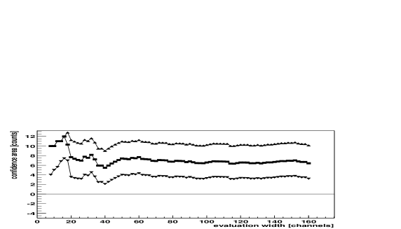
Figure 9: Upper part: Analysis of simulated spectrum with Gaussian peak of 5 events and FWHM of 9.4 channels on a Poisson-distributed background spectrum of 0.5 events/channel, as function of interval of analysis. The middle line is the best value. Upper and lower lines correspond to the 68.3$\%$ confidence limits. Lower part: The same as above, but the peak contains 20 events, the background is 4 events/channel. One channel corresponds to 0.36 keV in our measured spectra.

We further investigated with the computer-generated spectra the dependence of the peak analysis on the width of the energy range of evaluation. Two examples are shown in Fig. 9. Here the contents of the simulated peak found with the Bayes method is shown as function of the analysis interval given in channels (one channel corresponds to 0.36 keV in our measured spectra). The line in the middle is the best-fit value of the method, the upper and lower lines correspond to the upper and lower 68.3$\%$ confidence limits. In the upper figure the true number of counts in the simulated line was 5 events, on a Poisson-distributed background of 0.5 events/channel, in the lower figure it was 20 events on a background of 4 events/channel. It can be seen, that the analysis gives safely the correct number of counts, when choosing an analysis interval of not less than 40 channels.

3.3 Analysis of the Full Data

We first concentrate on the full spectra (see Fig. 5, and Fig.2 in KK-Evid01 ), without any data manipulation (no background subtraction, no pulse shape analysis). For the evaluation, we consider the raw data of the detectors.

The Bayesian peak finding procedure described in the last section leads to the result shown on the left hand sides of Figs. 13,13. For every energy E of the spectral range 2000 -2080 keV, we have determined the probability K_E that there is a line at E. All the remainder of the spectrum was considered to be background in this search.

The peak detection procedure yields lines at the positions of known Tabl-Isot96 weak $\gamma$-lines from the decay of ${}^{214}{Bi}$ at 2010.7, 2016.7, 2021.8 and 2052.9 keV. The lines at 2010.7 and 2052.9 keV are observed at a confidence level of 3.7 and 2.6$\sigma$, respectively. The observed intensities are consistent with the expectations from the strong Bi lines in our spectrum, and the branching ratios given in Tabl-Isot96 , within about the 2$\sigma$ experimental error (see Table 7 and KK-new02 ). The expectations here are calculated including summing effects, by Monte-Carlo simulation of our set-up. Only in this way the strong dependence of the relative intensities on the location of the impurities in the set-up can be properly taken into account (see Fig. 10). (A separate measurement with a ${}^{226}_{88}{Ra}$ source being in progress, will allow to study the intensities of the weak ${}^{214}{Bi}$ lines in the setup with high statistics).

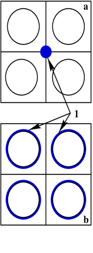
Figure 10: Demonstration of the dependence of the relative intensities of the weak ${}^{214}{Bi}$ lines on the location of the impurity in the experimental setup. The right side shows two different locations of the impurity (1) relative to the detectors. The left side shows the corresponding different relative intensities to be expected. Upper part: Source in some distance from the detectors (as in a) right part). Lower part: Source in copper cap very near around the detectors (as in b) right part). The ordinate shows relative intensities (see KK02 ).

	Intensity				Expect.	Expect.	Aalseth
Energy	of		Branching	Simul. of	rate	rate	et al.
(keV)	Heidelberg-	$\sigma$	RatiosTabl-Isot96	Experim.	accord.	accord.	(see Reply-Evid01 )
$*)$	Mos.Exper.		[$\%$]	Setup +)	to sim.**)	toTabl-Isot96 ++)	***)
609.312(7)	4399$\pm$92		44.8(5)	5715270$\pm$2400
1764.494(14)	1301$\pm$40		15.36(20)	1558717$\pm$1250
2204.21(4)	319$\pm$22		4.86(9)	429673$\pm$656
2010.71(15)	37.8$\pm$10.2	3.71	0.05(6)	15664$\pm$160	12.2$\pm$0.6	4.1$\pm$0.7	0.64
2016.7(3)	13.0$\pm$8.5	1.53	0.0058(10)	20027$\pm$170	15.6$\pm$0.7	0.5$\pm$0.1	0.08
2021.8(3)	16.7$\pm$8.8	1.90	0.020(6)	1606$\pm$101	1.2$\pm$0.1	1.6$\pm$0.5	0.25
2052.94(15)	23.2$\pm$9.0	2.57	0.078(11)	5981$\pm$115	4.7$\pm$0.3	6.4$\pm$1	0.99
2039.006	12.1$\pm$8.3	1.46

Table 7: ${}^{214}\rm{Bi}$ is product of the ${}^{238}\rm{U}$ natural decay chain through ${\beta}^{-}$ decay of ${}^{214}\rm{Pb}$ and $\alpha$ decay of ${}^{218}\rm{At}$. It decays to ${}^{214}\rm{Po}$ by ${\beta}^{-}$ decay. Shown in this Table are the measured intensities of ${}^{214}\rm{Bi}$ lines in the spectrum shown in Fig.1 of Ref. KK-Evid01 in the energy window 2000 - 2060 keV, our calculation of the intensities expected on the basis of the branching ratios given in Table of Isotopes Tabl-Isot96 , with and without simulation of the experimental setup, and the intensities expected by Aalseth et al. hep-ex/0202018, who do not simulate the setup and thus ignore summing of the $\gamma$ energies (see Reply-Evid01 ).
$*)$ We have considered for comparison the 3 strongest ${}^{214}\rm{Bi}$ lines, leaving out the line at 1120.287 keV (in the measured spectrum this line is partially overimposed on the 1115.55 keV line of ${}^{65}\rm{Zn}$). The number of counts in each line have been calculated by a maximum-likelihood fit of the line with a gaussian curve plus a constant background.
$+)$ The simulation is performed assuming that the impurity is located in the copper part of the detector chamber (best agreement with the intensities of the strongest lines in the spectrum). The error of a possible misplacement is not included in the calculation. The number of simulated events is $10^{8}$ for each of our five detectors.
$**)$ This result is obtained normalizing the simulated spectrum to the experimental one using the 3 strong lines listed in column one. Comparison to the neighboring column on the right shows that the expected rates for the weak lines can change strongly if we take into account the simulation. The reason is that the line at 2010.7 keV can be produced by summing of the 1401.50 keV (1.55%) and 609.31 keV (44.8%) lines, the one at 2016.7 keV by summing of the 1407.98 (2.8%) and 609.31 (44.8%) lines; the other lines at 2021.8 keV and 2052.94 keV do suffer only very weakly from the summing effect because of the different decay schemes.
$++)$ This result is obtained using the number of counts for the three strong lines observed in the experimental spectrum and the branching ratios from Tabl-Isot96 , but without simulation. For each of the strong lines the expected number of counts for the weak lines is calculated and then an average of the 3 expectations is taken.
***) Without simulation of the experimental setup. The numbers given here are close to those in the neighboring left column, when taking into account that Aalseth et al. refer to a spectrum which has only $\sim$11% of the statistics of the spectrum shown in Fig.1 of Ref. KK-Evid01 .

In addition, a line centered at 2039 keV shows up. This is compatible with the Q-value New-Q-2001 ; Old-Q-val of the double beta decay process. We emphasize, that at this energy no $\gamma$-line is expected according to the compilations in Tabl-Isot96 (see discussion in section 2). Figs. 13,13 do not show indications for the lines from ${}^{56}{Co}$ at 2034.7 keV and 2042 keV discussed earlier Diss-Dipl (but see also Fig. 14). We have at present no convincing identification of the lines around 2070 keV indicated by the peak identification procedure.

It may be important to note, that essentially the same lines as found by the peak scan procedure in Figs. 13,13,13, are found KK-Found02 ; KK-new02 when doing the same kind of analysis with the best existing natural Ge experiment of D. Caldwell et al. Caldw91 , which has a by a factor of $\sim$4 better statistics of the background. This experiment does, however, not see the line at 2039 keV (see section 3.5).

Bayesian peak detection (the same is true for Maximum Likelihood peak detection) of our data suggests a line at Q_ββ whether or not one includes detector Nr. 4 without muon shield (Figs. 13,13). The line is also suggested in Fig. 13 after removal of multiple site events (MSE), see below.

On the left-hand side of Figs. 13,13,13, the background intensity (1-$\eta$) identified by the Bayesian procedure is too high because the procedure averages the background over all the spectrum (including lines) except for the line it is trying to single out. Inclusion of the known lines into the fit naturally improves the background. As example, we show in Fig. 14 the spectrum of Fig. 5 (here in the original 0.36 keV binning) with a simultaneous fit of the range 2000 - 2060 keV (assuming lines at 2010.78, 2016.70, 2021.60, 2052.94, 2034.76, 2039.0, 2041.16 keV). The probability for a line in this fit at 2039 keV is 86%.

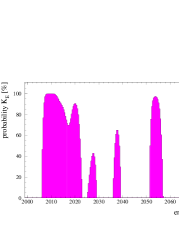
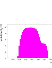
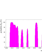
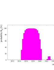
Figure 11: Scan for lines in the full spectrum taken from 1990-2000 with detectors Nr. 1,2,3,4,5, (Fig. 5), with the Bayesian method of sec. 3.1. The ordinate is the probability K_E that a line exists as defined in the text. Left: Energy range 2000 - 2080 keV.                   Right: Energy range of analysis $\pm\,5\sigma$ around Q_ββ.

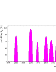
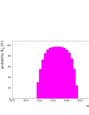
Figure 12: Left: Probability K_E that a line exists at a given energy in the range of 2000-2080 keV derived via Bayesian inference from the spectrum taken with detectors Nr. 1,2,3,5 over the period August 1990 to May 2000, 46.502 kg y (see Fig.2 from KK-Evid01 .) Right: Result of a Bayesian scan for lines as in the left part of this figure, but in the energy range of analysis $\pm\,5\sigma$ around Q_ββ.

Figure 13: Scan for lines in the single site event spectrum taken from 1995-2000 with detectors Nr. 2,3,5, (Fig. 5), with the Bayesian method (as in Figs. 13,13). Left: Energy range 2000 -2080 keV. Right: Energy range of analysis $\pm\,4.4\sigma$ around Q_ββ.

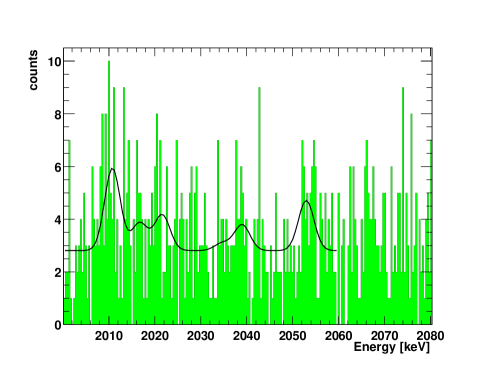
Figure 14: Simultaneous analysis of the spectrum measured with the ${}^{76}{Ge}$ detectors Nr. 1,2,3,4,5 over the period August 1990 - May 2000 (54.9813 kg y) (same as in Fig. 5, but here shown in the 0.36 keV original binning) in the energy range 2000 - 2060 keV, with the Maximum Likelihood Method. The probability for a line at 2039.0 keV found is this way is 86%.

Finally, on the right-hand side of Figs. 13,13 (and also Fig. 13) the peak detection procedure is carried out within an energy interval that seems to not contain (according to the left-hand side) lines other than the one at Q_ββ. This interval is broad enough (about $\pm$ 5 standard deviations of the Gaussian line, i.e. as typically used in search for resonances in high-energy physics) for a meaningful analysis (see Fig. 9 in section 3.2). We find, with the Bayesian method, the probability K_E = 96.5$\%$ that there is a line at 2039.0 keV is the spectrum shown in Fig. 5. This is a confidence level of 2.1 $\sigma$ in the usual language. The number of events is found to be 0.8 to 32.9 (7.6 to 25.2) with 95% (68%) c.l., with best value of 16.2 events. For the spectrum shown in Fig. 2 in KK-Evid01 , we find a probability for a line at 2039.0 keV of 97.4$\%$ (2.2 $\sigma$). In this case the number of events is found to be 1.2 to 29.4 with 95$\%$ c.l.. It is 7.3 to 22.6 events with 68.3$\%$ c.l.. The most probable number of events (best value) is 14.8 events. These values are stable against small variations of the interval of analysis, as expected from Fig. 9 in section 3.2. For example, changing the lower and upper limits of the interval of analysis between 2030 and 2032 and 2046 and 2050 yields consistently values of K_E between 95.3 and 98.5$\%$ (average 97.2$\%$) for the spectrum of Fig.2 of KK-Evid01 .

We also applied the Feldman-Cousins method recommended by the Particle Data Group Feldm98 ; RPD00 . This method (which does not use the information that the line is Gaussian) finds a line at 2039 keV on a confidence level of 3.1 $\sigma$ (99.8$\%$ c.l.).

3.4 Analysis of Single Site Events Data

From the analysis of the single site events (Fig. 5), we find after 28.053 kg y of measurement 9 SSE events in the region 2034.1 - 2044.9 keV ($\pm$ 3$\sigma$ around Q_ββ) (Fig. 15). Analysis of the single site event spectrum (Fig. 5), as described in

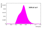
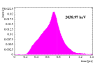
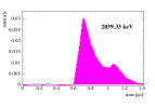
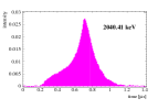
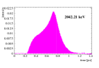
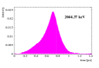
Figure 15: Events classified to be single site events (SSE) by all three methods of PSA in the range 2034.1 - 2044.9 keV, in the measurement period 10.1995 - 05.2000, 28.053 kg y.

section 3.1, shows again evidence for a line at the energy of Q_ββ (Fig. 13). Analyzing the range of 2032 - 2046 keV, we find the probability of 96.8$\%$ that there is a line at 2039.0 keV. We thus see a signal of single site events, as expected for neutrinoless double beta decay, precisely at the Q_ββ value obtained in the precision experiment of New-Q-2001 . The analysis of the line at 2039.0 keV before correction for the efficiency yields 4.6 events (best value) or (0.3 - 8.0) events within 95$\%$ c.l. ((2.1 - 6.8) events within 68.3$\%$ c.l.). Corrected for the efficiency to identify an SSE signal by successive application of all three PSA methods, which is 0.55 $\pm$ 0.10, we obtain a $0\nu\beta\beta$ signal with 92.4$\%$ c.l.. The signal is (3.6 - 12.5) events with 68.3$\%$ c.l. (best value 8.3 events). Thus, with proper normalization concerning the running times (kg y) of the full and the SSE spectra, we see that almost the full signal remains after the single site cut (best value), while the ${}^{214}{Bi}$ lines (best values) are considerably reduced. The reduction is comparable to the reduction of the 2103 keV and 2614 keV ${}^{228}{Th}$ lines (known to be multiple site or mainly multiple site), relative to the 1592 keV ${}^{228}{Th}$ line (known to be single site), see Fig. 16. The same reduction is also found for the strong ${}^{214}{Bi}$ lines (e.g. at 609.6 and 1763.9 keV (Fig. 16)).

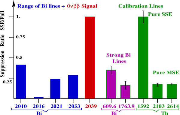
Figure 16: Relative suppression ratios: Remaining intensity after pulse shape analysis compared to the intensity in the full spectrum. Right: Result of a calibration measurement with a Th source - ratio of the intensities of the 1592 keV line (double escape peak, known to be 100% SSE), set to 1. The intensities of the 2203 keV line (single escape peak, known to be 100% MSE) as well as of the 2614 keV line (full energy peak, known to be dominantly MSE) are strongly reduced (error bars are $\pm 1\sigma$). The same order of reduction is found for the strong Bi lines occurring in our spectrum (see Fig. 3) - shown in this figure are the lines at 609.4 and 1763.9 keV. Left: The lines in the range of weak statistics around the line at 2039 keV (shown are ratios of best fit values). The Bi lines are reduced compared to the line at 2039 keV (set to 1), as to the 1592 keV SSE Th line.

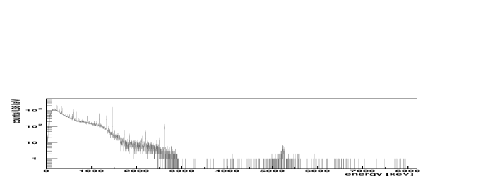
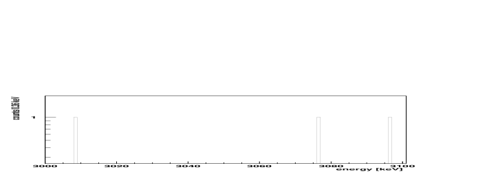
Figure 17: The measured sum spectrum up to $\sim$ 8 MeV (upper part) (22.36 kg y). No lines can be identified in the range 3-8 MeV, except a peak at 5.24$\pm$0.03 MeV, which we identify as $\alpha$ decay from ${}^{210}{Po}$ to ${}^{206}{Pb}$ (see Diss-Dipl ). Lower part: the range 3000 - 3100 keV, where the full energy peak should occur at 3061 keV, in case the 2039 keV signal would be the double escape peak of a $\gamma$-line.

The Feldman-Cousins method gives a signal at 2039.0 keV of 2.8 $\sigma$ (99.4$\%$). The possibility, that the single site signal at 2039.0 keV is the double escape line corresponding to a (much more intense!) full energy peak of a $\gamma$-line at 2039+1022=3061 keV is excluded from the high-energy part of our spectrum (see Fig. 17).

3.5 Comparison with Earlier Results

We applied the same methods of peak search as used in sections 3.3, 3.4, to the spectrum measured in the Ge experiment by Caldwell et al. Caldw91 more than a decade ago. These authors had the most sensitive experiment using natural Ge detectors (7.8% abundance of ${}^{76}{Ge}$). With their background being a factor of 9 higher than in the present experiment, and their measuring time of 22.6 kg y, they have a statistics for the background larger by a factor of almost 4 in their (very similar) experiment. This allows helpful conclusions about the nature of the background.

The peak scanning finds (Fig. 18) indications for peaks essentially at the same energies as in Figs. 13,13,13. This shows that these peaks are not fluctuations. In particular it sees the 2010.78 and 2052.94 keV ${}^{214}{Bi}$ lines with 3.6 and 2.8 $\sigma$ c.l., respectively. It finds, however, no line at Q_ββ (see also Fig. 19). This is consistent with the expectation from the rate found from the HEIDELBERG-MOSCOW experiment. About 17 observed events in the latter correspond to 0.6 expected events in the Caldwell experiment, because of the use of non-enriched material and the shorter measuring time.

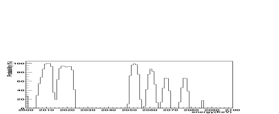
Figure 18: Peak scanning of the spectrum measured by Caldwell et al. Caldw91 with the Maximum Likelihood method (upper part), and with the Bayesian method (lower part) (as in Fig. 13,13,13) (see KK-new02 ).

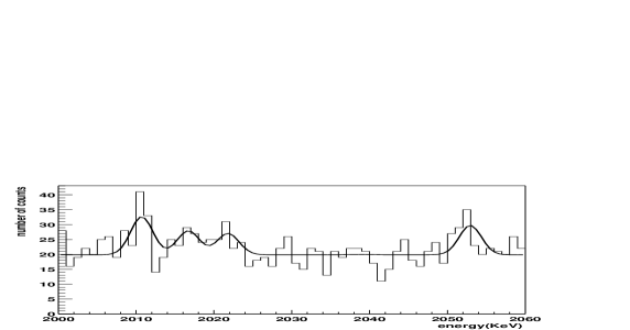
Figure 19: Analysis of the spectrum measured by D. Caldwell et al. Caldw91 , with the Maximum Likelihood Method, in the energy range 2000 - 2060 keV (as in Fig. 14) assuming lines at 2010.78, 2016.70, 2021.60, 2052.94, 2039.0 keV. In contrast to Fig. 14 no indication for a signal at 2039 kev is observed (see text).

Another Ge experiment (IGEX) using 9 kg of enriched ${}^{76}{Ge}$, but collecting since beginning of the experiment in the early nineties till shutdown in end of 1999 only 8.8 kg y of statistics DUM-RES-AVIGN-2000 , because of this low statistics also naturally cannot see any signal at 2039 keV.

3.6 Some Comments on the Bayesian, ${\chi}^{2}$ and
Maximum Likelihood Methods

We probed the sensitivity of peak identification for the three methods: Bayesian, ${\chi}^{2}$, Maximum-Likelihood, for the latter two using codes from Kchi-kvadr .

The disadvantage of the latter two methods is, that at low counting rates observation of lines with negative counting rate is possible. This is excluded in the Bayesian method. We find that the Bayesian method tends to systematically give too conservative confidence limits (see Table 5 in section 3.2). We shall discuss technical details of the three methods in a separate paper KK-new02 .

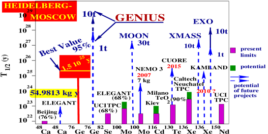
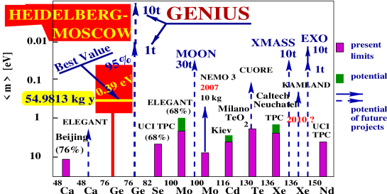
Figure 20: Present evidence for $0\nu\beta\beta$ decay from data of the HEIDELBERG-MOSCOW experiment and the potential of present and future $\beta\beta$ experiments. Vertical axis - half life limits (only HEIDELBERG-MOSCOW gives a value) in years, horizontal - isotopes used in the various experiments.

Figure 21: Present evidence for $0\nu\beta\beta$ decay from data of the HEIDELBERG-MOSCOW experiment and the potential of present and future $\beta\beta$ experiments. Vertical axis - effective neutrino mass limits (only HEIDELBERG-MOSCOW gives a value) in eV, horizontal - isotopes used in the various experiments.

4 Half-life of the Neutrinoless Mode and
Effective Neutrino Mass

We emphasize that we find in all analyses of our spectra a line at the value of Q_ββ. We have shown that to our present knowledge the signal at Q_ββ does not originate from a background $\gamma$-line. On this basis we translate the observed number of events into half-lives for the neutrinoless double beta decay. We give in Table 8 conservatively the values obtained with the Bayesian method and not those obtained with the Feldman-Cousins method. Also given in Table 8 are the effective neutrino masses $\langle m\rangle$ deduced using the matrix elements of Sta90 ; Mut89 .

We derive from the data taken with 46.502 kg y the half-life ${\rm T}_{1/2}^{0\nu}=(0.8-18.3)\times 10^{25}$ ${\rm y}$ (95$\%$ c.l.). The analysis of the other data sets, shown in Table 8 confirm this result. Of particular importance is that we see the $0\nu\beta\beta$ signal in the single site spectrum.

The result obtained is consistent with the limits given earlier by the HEIDELBERG-MOSCOW experiment HDM01 . It is also consistent with all other double beta experiments - which still reach less sensitivity (see Figs. 21,21). A second Ge-experiment DUM-RES-AVIGN-2000 , which has stopped operation in 1999 after reaching a significance of 9 kg y, yields (if one believes their method of ’visual inspection’ in their data analysis) in a conservative analysis a limit of ${\rm T}_{1/2}^{0\nu}>0.55\times 10^{25}{\rm~{}y}$ (90% c.l.). The ${}^{128}{Te}$ geochemical experiment Ber92 yields $\langle m_{\nu}\rangle<1.1$ eV (68 $\%$ c.l.), the ${}^{130}{Te}$ cryogenic experiment yields Ales00 $\langle m_{\nu}\rangle<1.8$ eV and the CdWO₄ experiment Dan2000 $\langle m_{\nu}\rangle<2.6$ eV, all derived with the matrix elements of Sta90 to make the results comparable to the present value.

Concluding we obtain, on the above basis, with more than 95$\%$ probability, first evidence for the neutrinoless double beta decay mode.

Significan-	Detectors	${\rm T}_{1/2}^{0\nu}{\rm~{}\,y}$	$\langle m\rangle$ eV	Conf.
ce $[kg\,y]$				level
54.9813	1,2,3,4,5	$(0.80-35.07)\times 10^{25}$	(0.08 - 0.54)	$95\%~{}c.l.$
		$(1.04-3.46)\times 10^{25}$	(0.26 - 0.47)	$68\%~{}c.l.$
		$1.61\times 10^{25}$	0.38	Best Value
46.502	1,2,3,5	$(0.75-18.33)\times 10^{25}$	(0.11 - 0.56)	$95\%~{}c.l.$
		$(0.98-3.05)\times 10^{25}$	(0.28 - 0.49)	$68\%~{}c.l.$
		$1.50\times 10^{25}$	0.39	Best Value
28.053	2,3,5 SSE	$(0.88-22.38)\times 10^{25}$	(0.10 - 0.51)	$90\%~{}c.l.$
		$(1.07-3.69)\times 10^{25}$	(0.25 - 0.47)	$68\%~{}c.l.$
		$1.61\times 10^{25}$	0.38	Best Value

Table 8: Half-life for the neutrinoless decay mode and deduced effective neutrino mass from the HEIDELBERG-MOSCOW experiment.

$M^{0\nu}$ from	Mut89 ; Sta90	Tom91	Hax84	Cau96	FaesSimc97	Sim99	Faes01	St-KK01-1 ; St-KK01-2
$\langle m\rangle$ eV 95$\%$	0.39	0.37	0.34	1.06	0.87	0.60	0.53	0.44 - 0.52

Table 9: The effect of nuclear matrix elements on the deduced effective neutrino masses. Shown are the neutrino masses deduced from the best value of ${\rm T}_{1/2}^{0\nu}=1.5\times 10^{25}{\rm~{}y}$ determined in this work with 97$\%$ c.l. when using matrix elements from various calculations and a phase factor of $F^{0\nu}_{1}=6.31\times{10}^{-15}\,y^{-1}$.

As a consequence, at this confidence level, lepton number is not conserved. Further our result implies that the neutrino is a Majorana particle. Both of these conclusions are independent of any discussion of nuclear matrix elements.

The matrix element enters when we derive a value for the effective neutrino mass. If using the nuclear matrix element from Sta90 ; Mut89 , we conclude from the various analyses given above the effective mass $\langle m\rangle$ to be $\langle m\rangle$ = (0.11 - 0.56) eV (95$\%$ c.l.), with best value of 0.39 eV. Allowing conservatively for an uncertainty of the nuclear matrix elements of $\pm$ 50$\%$ (for detailed discussions of the status of nuclear matrix elements we refer to Mut88 ; Gro89/90 ; Tom91 ; FaesSimc ; KK60Y ; Vog2001 ; Faes01 ; St-KK01-1 ; St-KK01-2 ) this range may widen to $\langle m\rangle$ = (0.05 - 0.84) eV (95$\%$ c.l.). In Table 9 we demonstrate the situation of nuclear matrix elements by showing the neutrino masses deduced from different calculations. It should be noted that the value obtained in Large Scale Shell Model Calculations Cau96 is understood to be too large by almost a factor of 2 because of the two small configuration space, (see, e.g. FaesSimc ), and that the second highest value given (from FaesSimc97 ), has now been reduced to 0.53 eV Faes01 . The recent studies by St-KK01-1 ; St-KK01-2 yield an effective mass of (0.44 - 0.52) eV. We see that the early calculations Sta90 done in 1989 agree within less than 25$\%$ with the most recent values.

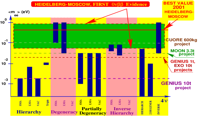
Figure 22: The impact of the evidence obtained for neutrinoless double beta decay in this paper (best value of the effective neutrino mass $\langle m\rangle$ = 0.39 eV, 95$\%$ confidence range (0.05 - 0.84) eV - allowing already for an uncertainty of the nuclear matrix element of a factor of $\pm$ 50$\%$) on possible neutrino mass schemes. The bars denote allowed ranges of $\langle m\rangle$ in different neutrino mass scenarios, still allowed by neutrino oscillation experiments. Hierarchical models are excluded by the new $0\nu\beta\beta$ decay result. Also shown are the expected sensitivities for the future potential double beta experiments CUORE, MOON, EXO and the 1 ton and 10 ton project of GENIUS KK-00-NOON-NOW-NANP-Bey97-GEN-prop (from KK-Sar_Evid01 ).

In the above conclusion for the effective neutrino mass, it is assumed that contributions to $0\nu\beta\beta$ decay from processes other than the exchange of a Majorana neutrino (see, e.g. KK60Y ; Moh91 and section 1) are negligible. It has been discussed, however, recently Ueh02-Ev that the possibility that $0\nu\beta\beta$ decay is caused by R-parity violation, may experimentally not be excluded, although this would require making R-parity violating couplings generation-dependent.

5 Conclusions and Outlook

With the value deduced for the effective neutrino mass, the HEIDELBERG-MOSCOW experiment excludes several of the neutrino mass scenarios allowed from present neutrino oscillation experiments (see Fig. 22) - allowing mainly only for degenerate mass scenarios, and an inverse hierarchy 3$\nu$ and 4$\nu$- scenario (the former of these being, however, strongly disfavored by a recent analysis of SN1987A Minak-Nuno ). For details we refer to KK-Sar_Evid01 . In particular, hierarchical mass schemes are excluded at the present level of accuracy.

According to Barg02-Sol a global analysis of all solar neutrino data including the recent SNO neutral-current rate selects the Large Mixing Angle (LMA) at the 90% c.l., however, the LOW solution is also viable, with 0.89 goodness of fit.

Assuming the degenerate scenario to be realized in nature we fix - according to the formulae derived in KKPS1-2 - the common mass eigenvalue of the degenerate neutrinos to m = (0.05 - 3.4) eV. Part of the upper range is already excluded by tritium experiments, which give a limit of m $<$ 2.2 eV, or 2.8 eV (95$\%$ c.l.) Trit00 . The full range can only partly (down to $\sim$ 0.5 eV) be checked by future tritium decay experiments, but could be checked by some future $\beta\beta$ experiments (see, e.g. KK60Y ; KK-00-NOON-NOW-NANP-Bey97-GEN-prop ). The deduced 95$\%$ interval for the sum of the degenerate neutrino masses is consistent with the range for $\Omega_{\nu}$ deduced from recent cosmic microwave background measurements and large scale structure (redshift) surveys, which still allow for a $\sum_{i}m_{i}\leq 4.4$ eV Teg00 ; Wang02 . The range of $\langle m\rangle$ fixed in this work is, already now, in the range to be explored by the satellite experiments MAP and PLANCK Lop ; KK-China01 (see Fig. 23). It lies in a range of interest for Z-burst models recently discussed as explanation for super-high energy cosmic ray events beyond the GKZ-cutoff Farj00-04keV ; PW01-Wail99 ; Fodor02-Evid . Finally, the deduced best value for the mass is consistent with expectations from experimental $\mu~{}\to~{}e\gamma$ branching limits in models assuming the generating mechanism for the neutrino mass to be also responsible for the recent indication for an anomalous magnetic moment of the muon MaRaid01 . A recent model with underlying A₄ symmetry for the neutrino mixing matrix (and the quark mixing matrix) also leads to degenerate neutrino masses consistent with the present experiment BMV02-Evid . This model succeeds to consistently describe the large (small) mixing in the neutrino (quark) sector.

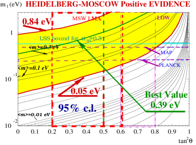
Figure 23: Double beta decay observable $\langle m\rangle$ and oscillation parameters: The case for degenerate neutrinos. Plotted on the axes are the overall scale of neutrino masses $m_{0}$ and mixing $\tan^{2}\,\theta_{12}$. Also shown is a cosmological bound deduced from a fit of CMB and large scale structure Lop and the expected sensitivity of the satellite experiments MAP and PLANCK. The present limit from tritium $\beta$ decay of 2.2 eV Trit00 would lie near the top of the figure. The range of $\langle m\rangle$ fixed by the HEIDELBERG-MOSCOW experiment is, in the case of small solar neutrino mixing, already in the range to be explored by MAP and PLANCK.

The neutrino mass deduced leads to 0.002 $\,\leq\Omega_{\nu}h^{2}\leq\,0.1$, and thus may allow neutrinos to still play an important role as hot dark matter in the Universe (see also Barg02-Ev ).

With the HEIDELBERG-MOSCOW experiment, the era of the small smart experiments is over. New approaches and considerably enlarged experiments (as discussed, e.g. in KK60Y ; KK-LeptBar98 ; KK-00-NOON-NOW-NANP-Bey97-GEN-prop ; KK-NANP01-TAUP01 ) will be required in future to fix the neutrino mass with higher accuracy.

Since it was realized in the HEIDELBERG-MOSCOW experiment, that the remaining small background is coming from the material close to the detector (holder, copper cap, …), elimination of any material close to the detector will be decisive. Experiments which do not take this into account, like, e.g. CUORE Ales00 , and MAJORANA MAJOR-WIPP00 , will allow only rather limited steps in sensitivity.

Another crucial point is - see eq. (6) - the energy resolution, which can be optimized only in experiments using Germanium detectors or bolometers. It will be difficult to probe evidence for this rare decay mode in experiments, which have to work - as result of their limited resolution - with energy windows around Q_ββ of up to several hundreds of keV, such as NEMO III ApPec02 , EXO EXO-LowNu2 , CAMEO CAMEO-Taup01 .

For example - according to eq. (6) - to compensate for the projected energy resolution of only 130 keV of EXO EXO-LowNu2 , the mass of the EXO experiment has to be increased to almost half a ton of enriched material, to reach the sensitivity of the HEIDELBERG-MOSCOW experiment. Only after that one can think about improving the sensitivity, by improving the background. Correspondingly, according to eq. (6), a potential future 100 kg ${}^{82}{Se}$ NEMO experiment would be because of its low efficiency, equivalent only to a 10 kg experiment (not talking about the energy resolution).

In the first proposal for a third generation double beta experiment, the GENIUS proposal KK-Neutr98 ; KK-00-NOON-NOW-NANP-Bey97-GEN-prop , the idea is to use ’naked’ Germanium detectors in a huge tank of liquid nitrogen. It seems to be at present the only proposal, which can fulfill both requirements mentioned above. The potential of GENIUS is together with that of some later proposals indicated in Fig. 22. GENIUS would - with only 100 kg of enriched ${}^{76}{Ge}$ - increase the confidence level of the present $0\nu\beta\beta$ signal to 5$\sigma$ within one year of measurement. A GENIUS Test Facility is at present under construction in the GRAN SASSO Underground Laboratory GENIUS-TF02 .

6 Acknowledgments

The authors are indebted to C. Tomei and C. Dörr for their help in the analysis of the Bi lines, to H.L. Harney for cooperation on the Bayes method, and to M. Zavertiaev for many inspiring discussions.

References

- (1) H.V. Klapdor-Kleingrothaus, A. Dietz, H.V. Harney and I.V. Krivosheina, Modern Physics Letters A 16, No. 37, 2409-2420 (2001) and hep-ph/ 0201231.
- (2) H.V. Klapdor, Vorschlag eines Experiments, Internal Report MPI H V 17, 18pp. (1987).
- (3) H.V. Klapdor-Kleingrothaus and U. Sarkar, Modern Physics Letters A 16, No. 38, 2469-2482 (2001).
- (4) H.V. Klapdor-Kleingrothaus, hep-ph/0205228.
- (5) H.V. Klapdor-Kleingrothaus, H. Päs and A.Yu. Smirnov, Phys. Rev. D 63, 073005 (2001), and hep-ph/0003219 (2000) and hep-ph/0103076 (2001), and in Proc. of 3rd International Conference on Dark Matter in Astro and Particle Physics (Dark 2000), Heidelberg, Germany, 10-16 July, 2000, ed. H.V. Klapdor-Kleingrothaus, Springer, Heidelberg (2001) 420 - 434.
- (6) H.V. Klapdor-Kleingrothaus, “60 Years of Double Beta Decay - From Nuclear Physics to Beyond the Standard Model”, World Scientific, Singapore (2001) 1281 pp.
- (7) E. Majorana, Nuovo Cimento 14, 171 - 184 (1937).
- (8) G. Racah, Nuovo Cimento 14, 322 - 328 (1937).
- (9) W.H. Furry, Phys. Rev. 56, 1184 - 1193 (1939).
- (10) J. A. Mclennan, Jr. Phys. Rev. 106, 821 (1957).
- (11) K. M. Case, Phys. Rev. 107, 307 (1957).
- (12) D. V. Ahluwalia, Int. J. Mod. Phys. A 11, 1855 (1996).
- (13) J. Schechter and J.W.F. Valle, Phys. Rev. D 25, 2951 - 2954 (1982).
- (14) H. Päs, M. Hirsch, H.V. Klapdor-Kleingrothaus and S.G. Kovalenko, Phys. Lett. B 453, 194-198 (1999).
- (15) M. Hirsch and H.V. Klapdor-Kleingrothaus, Phys. Lett. B 398, 311 (1997); Phys. Rev. D 57, 1947 (1998); M. Hirsch, H.V. Klapdor-Kleingrothaus and St. Kolb, Phys. Rev. D 57, 2020 (1998).
- (16) HEIDELBERG-MOSCOW Collaboration (M. Günther et al.), Phys. Rev. D 55, 54 (1997).
- (17) HEIDELBERG-MOSCOW Collaboration, Phys. Lett. B 407, 219 - 224 (1997).
- (18) HEIDELBERG–MOSCOW Collaboration, Phys. Rev. Lett. 83, 41 - 44 (1999).
- (19) H.V. Klapdor-Kleingrothaus et al.,(HEIDELBERG-MOSCOW Collaboration), Eur. Phys. J. A 12 (2001) 147 and hep-ph/0103062, in Proc. of ”Third International Conference on Dark Matter in Astro- and Particle Physics”, DARK2000 H.V. Klapdor-Kleingrothaus (Editor), Springer-Verlag Heidelberg, (2001) 520 - 533.
- (20) H.V. Klapdor-Kleingrothaus et al.,(HEIDELBERG-MOSCOW Collaboration), Erratum Eur. Phys. J. (2002).
- (21) H.V. Klapdor-Kleingrothaus, in Proc. of 18th Int. Conf. on NEUTRINO 98, Takayama, Japan, 4-9 Jun 1998, (eds) Y. Suzuki et al. Nucl. Phys. Proc. Suppl. 77, 357 - 368 (1999).
- (22) H.V. Klapdor-Kleingrothaus, in Proc. of the Int. Symposium on Advances in Nuclear Physics, eds.: D. Poenaru and S. Stoica, World Scientific, Singapore (2000) 123 - 129.
- (23) H.V. Klapdor-Kleingrothaus, in Proc. of the 17th International Conference ‘ ‘Neutrino Physics and Astrophysics”, NEUTRINO’96, Helsinki, Finland, June 13 - 19, 1996, eds. K. Enqvist, K. Huitu and J. Maalampi, World Scientific, Singapore, (1997) 317 - 341.
- (24) M. Doi, T. Kotani and E. Takasugi, Prog. of Theor. Phys. Suppl. 83 (1985) 1 - 175.
- (25) K. Muto and H.V. Klapdor, in “Neutrinos”, Graduate Texts in Contemporary Physics”, ed. H.V. Klapdor, Berlin, Germany: Springer (1988) 183 - 238.
- (26) K. Grotz and H.V. Klapdor, “Die Schwache Wechselwirkung in Kern-, Teilchen- und Astrophysik”, B.G. Teubner, Stuttgart (1989), “The Weak Interaction in Nuclear, Particle and Astrophysics”, IOP Bristol (1990), Moscow, MIR (1992) and China (1998).
- (27) H.V. Klapdor-Kleingrothaus and A. Staudt, “Teilchenphysik ohne Beschleuniger”, B.G. Teubner, Stuttgart (1995), “Non–Accelerator Particle Physics”, IOP Publishing, Bristol and Philadelphia (1995) and 2. ed. (1998) and Moscow, Nauka, Fizmalit (1998), translated by V.A. Bednyakov.
- (28) P.Vogel in it“Current Aspects of Neutrino Physics”, ed. D.O. Caldwell, Berlin, Heidelberg, Germany: Springer (2001) 177 - 198.
- (29) H.V. Klapdor-Kleingrothaus, Int. J. Mod. Phys. A 13 (1998) 3953 and in Proc. of Int. Symposium on Lepton and Baryon Number Violation, Trento, Italy, 20-25 April, 1998, ed. H.V. Klapdor-Kleingrothaus and I.V. Krivosheina, IOP, Bristol, (1999) 251-301 and Preprint: hep-ex/9901021.
- (30) H.V. Klapdor-Kleingrothaus, Springer Tracts in Modern Physics, 163 (2000) 69-104, Springer-Verlag, Heidelberg, Germany (2000).
- (31) W.C. Haxton and G.J. Stephenson, Prog. Part. Nucl. Phys. 12, 409 - 479 (1984).
- (32) K. Muto, E. Bender and H.V. Klapdor, Z. Phys. A 334, 177 - 186 (1989).
- (33) A. Staudt, K. Muto and H.V. Klapdor-Kleingrothaus, Eur. Phys. Lett. 13, 31 - 36 (1990).
- (34) T. Tomoda, Rept. Prog. Phys. 54, 53 - 126 (1991).
- (35) E. Caurier, F. Nowacki, A. Poves and J. Retamosa, Phys. Rev. Lett. 77, 1954 - 1957 (1996).
- (36) F. Šimkovic et al., Phys. Lett. B 393, 267 - 273 (1997).
- (37) A. Faessler and F. Simkovic, J. Phys. G 24, 2139 - 2178 (1998).
- (38) F. Šimkovic, G. Pantis, J.D. Vergados and A. Faessler, Phys. Rev. C 60, 055502 (1999).
- (39) S. Stoica and H.V. Klapdor-Kleingrothaus, Eur. Phys. J. A 9, 345 (2000).
- (40) S. Stoica and H.V. Klapdor-Kleingrothaus, Nucl. Phys. A 694, 269-294 (2001).
- (41) S. Stoica and H.V. Klapdor-Kleingrothaus, Phys. Rev. C 63, 064304 (2001).
- (42) F. Simkovic et al., Phys. Rev. C 64, 035501(2001).
- (43) F. Vissani, in Proc. of 3rd International Conference on Dark Matter in Astro and Particle Physics (Dark 2000), Heidelberg, Germany, 10-16 July, 2000, ed. H.V. Klapdor-Kleingrothaus, Springer, Heidelberg (2001) 435 - 447.
- (44) H. Georgi und S.L. Glashow, Phys. Rev. D 61 (2000) 097301 and hep-ph/9808293.
- (45) J. Ellis and S. Lola, Phys. Lett. B 458, 310 (1999) and hep-ph/ 9904279.
- (46) R. Adhikari and G. Rajasekaran, Phys. Rev. D 61, 031301(R) (1999).
- (47) H. Minakata and H. Nunokawa, Phys. Lett. B 504 301 - 308 (2001) and hep-ph/ 0010240.
- (48) H. Minakata in hep-ph/0101148.
- (49) H. Minakata and O. Yasuda, Phys. Rev. D 56, 1692 (1997) and hep-ph/ 9609276.
- (50) J.H. Bahcall, M.C. Gonzalez-Garcia and C.Pena-Garay, hep-ph/0106258 and CERN-TH/2001-165.
- (51) V. Barger et al., Phys. Lett. B 537 (2002) 179-186 and hep-ph/0204253.
- (52) H.V. Klapdor-Kleingrothaus and U. Sarkar, to be publ. Phys. Lett. B (2002) and hep-ph/0201226; and Phys. Lett. B 532 71 - 76 (2002) and hep-ph/0202006.
- (53) E. Ma, Mod. Phys. Lett. A 17 (2002) 289-294, and hep-ph/0201225.
- (54) V. Barger, S.L. Glashow, D. Marfatia and K. Whisnant, Phys. Lett. B 532 (2002) 15-18, and hep-ph/0201262.
- (55) Y. Uehara, Phys. Lett. B 537 (2002) 256-260, hep-ph/ 0201277; hep-ph/ 0205294.
- (56) H.Minakata and H. Sugiyama, Phys. Lett. B 532 (2002) 275-283, and hep-ph/0202003.
- (57) U. Chattopadhyay et al., hep-ph/0201001.
- (58) Zhi-zhong Xing, Phys. Rev. D 65 (2002) 077302, and hep-ph/0202034.
- (59) T. Hambye, hep-ph/0201307.
-
(60)
D.V. Ahluwalia and M. Kirchbach, hep-ph/0204144 and
to be publ. Phys. Lett. B (2002);
Phys. Lett. B 529 (2002) 124 - 131 and
hep-th/0202164;
and gr-qc/0207004. - (61) E. Witten, Nature 415 (2002) 969 - 971.
- (62) B. Brahmachari and E. Ma, Phys. Lett. B 536 (2002) 259-262, and hep-ph/0202262.
- (63) N. Haba and T. Suzuki, Mod. Phys. Lett A 17 (2002) 865-874 and hep-ph/0202143; and hep-ph/0205141.
- (64) B. Brahmachari, S. Choubey and R.N. Mohapatra, Phys. Lett. B 536 (2002) 94-100 and hep-ph/0204073.
- (65) G. Barenboim et al., Phys. Lett. B 537 (2002) 227, and hep-ph/0203261.
- (66) Z. Fodor, S.D. Katz and A. Ringwald, JHEP 0206 (2002) 046 and hep-ph/0203198.
- (67) S. Pakvasa and P. Roy, Phys. Lett. B 535 (2002) 181-186, and hep-ph/0203188.
- (68) H.B. Nielsen and Y. Takanishi, hep-ph/0110125; and Nucl. Phys. B 636 (2002) 305-337 and hep-ph/0204027.
- (69) D.A. Dicus, H-J. He, and J.N. Ng, Phys. Lett. B 537 (2002) 83-93, and hep-ph/0203237.
- (70) A.S. Joshipura and S.D. Rindani, hep-ph/0202064.
- (71) G.C. Branco et al., hep-ph/0202030.
- (72) M-Y. Cheng and K. Cheung, hep-ph/0203051.
- (73) M. Frigerio and A.Yu. Smirnov, hep-ph/0202247.
- (74) K. Matsuda et al., hep-ph/0204254.
- (75) F. Feruglio et al., hep-ex/0201291.
- (76) B. Maier, Dipl. Thesis, Univ. Heidelberg, 1993, and Dissertation, November 1995, MPI-Heidelberg; F. Petry, Dissertation, November 1995, MPI-Heidelberg; J. Hellmig, Dissertation, November 1996, MPI-Heidelberg; B. Majorovits, Dissertation, December 2000, MPI-Heidelberg; A. Dietz, Dipl. Thesis, Univ. Heidelberg, 2000 (unpublished), and Dissertation, in preparation.
- (77) G. Douysset et al., Phys. Rev. Lett. 86, 4259 - 4262 (2001).
- (78) J.G. Hykawy et al., Phys. Rev. Lett. 67, 1708 (1991).
- (79) R.B. Firestone and V.S. Shirley, Table of Isotopes, Eighth Edition, John Wiley and Sons, Incorp., N.Y. (1998) and S.Y.F. Chu, L.P. Ekström and R.B. Firestone The Lund/LBNL Nuclear Data Search, Vers.2.0, Febr.1999; and http://nucleardata.nuclear.lu.se/nucleardata/toi/radSearch.asp
- (80) J. Hellmig and H.V. Klapdor-Kleingrothaus, Nucl. Instrum. Meth. A 455, 638 - 644 (2000).
- (81) J. Hellmig, F. Petry and H.V. Klapdor-Kleingrothaus, Patent DE19721323A.
- (82) B. Majorovits and H.V. Klapdor-Kleingrothaus. Eur. Phys. J. A 6, 463 (1999).
- (83) C.M. Baglin, S.Y.F. Chu, J. Zipkin, Table of isotopes, eight edition, J. Wiley & Sons, Inc. (1996.)
- (84) W. Struve, Nucl. Phys. 222, 605 (1973).
- (85) F. Areodo, Il Nuovo Cimento 112A, 819 (1999).
- (86) H. Liljavirta, Phycica Scripta 18, 75 (1978).
- (87) G. D’Agostini, hep-ex/0002055, W. von der Linden and V. Dose, Phys. Rev. E 59 6527 (1999), and F.H. Fröhner, JEFF Report 18 NEA OECD (2000) and Nucl. Sci. a. Engineering 126 (1997) 1.
- (88) G.J. Feldman, R.D. Cousins, Phys. Rev. D 57 (1998) 3873.
- (89) D.E Groom et al., Particle Data Group, Eur. Phys. J. C 15, 1 (2000).
- (90) R.M. Barnett et al., Particle Data Group, Phys. Rev. D 54, 1 (1996).
- (91) A. O’Hagan, “Bayesian Inference”, Vol. 2B of Kendall’s Advanced Theory of Statistics, Arnold, London (1994).
- (92) http://root.cern.ch/
- (93) http://wwwinfo.cern.ch/asd/lhc++/indexold.html
- (94) R.N. Mohapatra and P.B. Pal, “Massive Neutrinos in Physics and Astrophysics”, Singapore, Singapore: World Scientific, World Scientific lecture notes in physics, 41 (1991) 318 pp.
- (95) C. Weinheimer, in Proc. of 3rd International Conference on Dark Matter in Astro and Particle Physics (Dark 2000), Heidelberg, Germany, 10-16 July, 2000, ed. H.V. Klapdor-Kleingrothaus, Springer, Heidelberg (2001) 513 - 519.
- (96) H.V. Klapdor-Kleingrothaus, hep-ph/0103074 and in Proc. of 2nd Workshop on Neutrino Oscillations and Their Origin (NOON 2000), Tokyo, Japan, 6-18 Dec. 2000, ed: Y. Suzuki et al., World Scientific (2001). H.V. Klapdor-Kleingrothaus, Nucl. Phys. Proc. Suppl. 100, 309 - 313 (2001) and hep-ph/ 0102276. H.V. Klapdor-Kleingrothaus, Part. Nucl. Lett. 104, 20 - 39 (2001) and hep-ph/ 0102319. H.V. Klapdor-Kleingrothaus in Proceedings of BEYOND’97, First International Conference on Particle Physics Beyond the Standard Model, Castle Ringberg, Germany, 8-14 June 1997, edited by H.V. Klapdor-Kleingrothaus and H. Päs, IOP Bristol (1998) 485 - 531. H.V. Klapdor-Kleingrothaus et al. MPI-Report MPI-H-V26-1999 and Preprint: hep-ph/9910205 and in Proceedings of the 2nd Int. Conf. on Particle Physics Beyond the Standard Model BEYOND’99, Castle Ringberg, Germany, 6-12 June 1999, edited by H.V. Klapdor-Kleingrothaus and I.V. Krivosheina, IOP Bristol, (2000) 915 - 1014. H.V. Klapdor-Kleingrothaus, Nucl. Phys. B 110 58-60 (2002), Proc. of TAUP’01 (2002), Gran-Sasso, Italy, September 7-13, 2001, eds A. Bettini et al.
- (97) E. Ma and M. Raidal, Phys. Rev. Lett. 87 (2001) 011802; Erratum-ibid. 87 (2001) 159901 and hep-ph/0102255;
- (98) K.S. Babu, E. Ma and J.W.F. Valle, hep-ph/0206292 v.1.
- (99) D. Fargion et al., in Proc. of DARK2000, Heidelberg, Germany, July 10-15, 2000, Ed. H.V. Klapdor-Kleingrothaus, Springer, Heidelberg, (2001) 455 - 468.
- (100) T.J. Weiler, in Proc. Beyond the Desert 1999, Accelerator, Non-Accelerator and Space Approaches, Ringberg Castle, Tegernsee, Germany, 6-12 Juni 1999, edited by H.V. Klapdor–Kleingrothaus and I.V. Krivosheina, IOP Bristol, (2000) 1085 - 1106; H. Päs and T.J. Weiler, Phys. Rev. D 63 (2001) 113015, and hep-ph/0101091.
- (101) H.V. Klapdor-Kleingrothaus, Part. Nucl. Lett. No. 1 [104] (2001) 20-39, and H.V. Klapdor-Kleingrothaus, Nucl. Phys. B 110 (2002) 364-368, Proc. of TAUP’01 (2002), Gran-Sasso, Italy, September 7-13, 2001, eds A. Bettini et al.
- (102) R.E. Lopez, astro-ph/9909414; J.R. Primack and M.A.K. Gross, astro-ph/0007165; J.R. Primack, astro-ph/0007187; J. Einasto, in Proc. of DARK2000, Heidelberg, Germany, July 10-15, 2000, Ed. H.V. Klapdor-Kleingrothaus, Springer, Heidelberg (2001) 3 - 11.
- (103) X. Wang, M. Tegmark and M. Zaldarriaga, Phys. Rev. D 65 (2002) 123001 and astro-ph/ 0105091.
- (104) M. Tegmark et al., hep-ph/0008145.
- (105) H.V. Klapdor-Kleingrothaus, in Proc. of Intern. Conf. “Flavor Physics”, ICFP01, 31 May - 6 June, 2001, Zhang-Jia-jie, China, ed. by Y.-L. Wu, World Scientific, Singapure (2002) 93 - 110.
-
(106)
H.V. Klapdor-Kleingrothaus et al.,
Part. and Nucl. Lett. 110, No 1 (2002) 57-79;
and in Proc. of BEYOND 2002, Oulu, Finland, June 2002, eds. (IOP, Bristol and Philadelphia, 2002), eds. H.V. Klapdor-Kleingrothaus et al.;
and H.V. Klapdor-Kleingrothaus et al., to be publ. (2002). - (107) H.V. Klapdor-Kleingrothaus et al., Found. of Phys. 32, No 8 (2002) 1181 - 1223.
- (108) A. Dietz, Dissertation, (2003) MPI-Heidelberg.
- (109) H.V. Klapdor-Kleingrothaus et al., to be publ. (2002).
- (110) D. Caldwell, J. Phys. G 17, S137-S144 (1991).
- (111) T. Bernatowicz, R. Cowsik, C. Hohenberg and F. Podosek, Phys. Rev. Lett. 69, 2341 - 2344 (1992) and Phys. Rev. C 47, 806 - 825 (1993).
- (112) F. A. Danevich et al., Phys. Rev. C 62, 045501 (2000).
- (113) CAMEO Collaboration in Proc. of Taup 2001, Gran Sasso, Italy, 8.-12. Sept. 2001 (editors A. Bettini et al.).
- (114) C.E. Aalseth et al. (IGEX Collaboration), Yad. Fiz. 63, No 7, 1299 - 1302 (2000).
- (115) L. DeBraekeleer, talk at Worksh. on the Next Generation U.S. Underground Science Facility, WIPP, June 12-14, 2000, Carlsbad, New Mexico, USA: C.E. Aalseth et al., Proc. Taup 2001, Gran Sasso, Italy, 8.-12. Sept. 2001 (editors A. Bettini et al.).
- (116) G. Gratta, talk given on ApPEC, Astroparticle Physics European Coordination, Paris, France 22.01.2002, and in Proc. of LowNu2, Dec. 4-5 (2000) Tokyo, Japan, ed: Y. Suzuki, World Scientific (2001) p.98.
- (117) (CUORE Coll.), talk given on ApPEC, Astroparticle Physics European Coordination, Paris, France 22.01.2002; A. Alessandrello et al., Phys. Lett. B 486, 13-21 (2000) and S. Pirro et al., Nucl. Instr. Methods A 444, 71-76 (2000).
- (118) X. Sarazin (for the NEMO Collaboration), talk given on ApPEC, Astroparticle Physics European Coordination, Paris, France 22.01.2002; (NEMO Collaboration), Contr. paper for XIX Int. Conf. NEUTRINO2000, Sudbury, Canada, June 16 - 21, 2000 LAL 00-31 (2000) 1 - 10 and (NEMO-III Collaboration) in Proc. of NANPino2000, Dubna, Russia, July 2000, ed. V. Bednjakov, Part. and Nucl. Lett. 3, 62 (2001).
- (119) H.V. Klapdor-Kleingrothaus et al., Nucl. Instr. Meth. A 481 (2002) 149-159.