Group projection method in statistical systems

Abstract

We discuss an application of group theoretical methods to the formulation of the thermodynamics of systems constrained by the conservation laws described by a semi–simple compact Lie group. A general projection method that allows to construct a partition function for a given irreducible representation of the Lie group is outlined. Applications of the method in Lattice Gauge Theory (LGT) for non–zero baryon number and in the phenomenological description of particle production in ultrarelativistic heavy ion collisions are also indicated.

1 Introduction

In the formulation of the thermodynamics of a strongly interacting medium one needs in general to implement the constraints imposed by the conservation laws that are governed by an internal symmetry of the Hamiltonian [1, 2, 3, 4, 5, 6, 7, 8]. In this paper, we discuss how applying the basic properties of the Lie groups and their representations one can derive the partition function that accounts for these constraints. We present examples of the application of the method for different statistical systems and phenomenological models.

2 Projected partition function

The usual way of treating the problem of quantum number conservation in statistical physics is by introducing the grand canonical partition function,

$$Z(\mu_{S},T,V)={\rm Tr}[e^{-\beta(\hat{H}-\mu_{S}\hat{S})}],$$ (1)

with $\hat{H}$ being the Hamiltonian, $\hat{S}$ the charge operator, $\beta$ the inverse temperature, $V$ the volume of the system and $\mu_{S}$ the chemical potential associated with the conserved charge $S$. The chemical potential in Eq. (1) plays the role of the Lagrange multiplier which is fixed by the condition that the charge is conserved on the average and has the required value $\langle S\rangle$ such that:

$$\langle S\rangle=T{{\partial\ln Z(\mu_{S},T)}\over{\partial\mu_{S}}}.$$ (2)

The grand canonical partition function (1) provides an adequate description of the statistical properties of the system only if the number of particles carrying charge $S$ is asymptotically large and if its fluctuations can be neglected.

In order to derive a more general statistical operator that is free from the above requirements one usually replaces the function (1) by the canonical partition function $Z_{S}$ that accounts for an exact charge conservation

$$Z_{S}(T,V):={\rm Tr_{S}}[e^{-\beta\hat{H}}].$$ (3)

The subscript $S$ under the trace indicates that it is restricted to the states that carry an exact value $S$ of the conserved charge. Obviously $Z_{S}(T,V)$ from Eq. (3) and $Z(\mu_{S},T,V)$ from Eq. (1) are connected via cluster decomposition

$$Z(\mu_{S},T,V)=\sum_{s=-\infty}^{s=+\infty}Z_{S}\lambda_{S}^{s},$$ (4)

with the fugacity parameter $\lambda_{S}:=e^{\beta\mu_{S}}$. Thus, $Z_{S}$ is viewed as a coefficient in the Laurent series of $Z$ in the fugacity. Applying the Cauchy formula in Eq. (4) one calculates $Z_{S}$ by taking an inverse transformation:

$$Z_{S}(T,V)=\int_{-\pi}^{+\pi}{{d\phi}\over{2\pi}}e^{-is\phi}\tilde{Z}(\phi,T,V).$$ (5)

The generating function $\tilde{Z}(\phi,T,V):=Z(\lambda_{S}=e^{i\phi},T,V)$ is obtained from the grand canonical partition function (1) by ”Wick rotation” of the chemical potential, $\mu_{S}\to i\phi$. The function $\tilde{Z}$ is unique for all canonical partition functions that are formulated for a fixed value of the conserved charge.

The integral (5) describes the projection onto the canonical partition function that accounts for an exact conservation of an abelian charge. This is the projection procedure as $Z_{S}$ is also obtained from

$$Z_{S}(T,V)={\rm Tr}[e^{-\beta\hat{H}}\hat{P}_{S}]$$ (6)

where $\hat{P}_{S}$ is the projection operator on the states with a given value of the conserved charge $S$. For an additive quantum numbers, $\hat{P}_{S}$ is just a delta function $P_{S}=\delta_{S^{,},S}\hat{I}$. Using the Fourier expression of $\delta_{S^{,},S}$ in Eq. (6) one reproduces the projected formula (5).

The conservation of an additive quantum number is usually related with an invariance of the Hamiltonian under the abelian U(1) internal symmetry group. In many physics applications it is of importance to generalize the projection method to symmetries that are related with a non-abelian Lie groups $G$. An example is a special unitary group SU(N) that plays an essential role in the strong interaction. A generalization of the projection method would require to specify the projection operator or the generating function. Consequently, the partition function obtained with a specific eigenvalue of the Casimir operator that fixes the multiplet of the irreducible representation of the symmetry group $G$ can be determined.

To find the generating function for the canonical partition function with respect to the symmetry group $G$, one introduces $\tilde{Z}(g)$ [1]

$$\tilde{Z}(g):={\rm Tr}[U(g)e^{-\beta\hat{H}}]$$ (7)

as the function on the group $G$ with U(g) being a unitary representation of the group and $g\in G$. The U(g) can be decomposed into irreducible representations $U_{\alpha}(g)$,

$$U(g)=\sum_{\alpha}^{\bigoplus}U_{\alpha}(g),$$ (8)

and thus, from Eqs. (7) and (8) one can write explicitly

$$\tilde{Z}(g): = \sum_{\alpha}{\rm Tr_{\alpha}}[U_{\alpha}(g)e^{-\beta\hat{H}}]$$ (9)

$$= \sum_{\alpha}\sum_{\nu_{\alpha},\xi_{\alpha}}\langle\nu_{\alpha},\xi_{\alpha}\mid U_{\alpha}(g)e^{-\beta\hat{H}}\mid\nu_{\alpha},\xi_{\alpha}\rangle,$$

where $\nu_{\alpha}$ labels the states within the representation $\alpha$ and $\xi_{\alpha}$ are degeneracy parameters of a given representation. Due to the requirement of an exact symmetry the only non–vanishing matrix elements of the evolution operator $e^{-\beta\hat{H}}$ are those diagonal in $\nu_{\alpha}$. The matrix elements of $U_{\alpha}(g)$ are non-zero if they are diagonal in $\xi_{\alpha}$. Finally, the matrix elements of the Hamiltonian are independent of the states within representation and those of $U(g)$ of degeneracy factors. Consequently, the matrix elements in Eq. (9) factorize and the generating function is

$$\tilde{Z}(g)=\sum_{\alpha}{{\chi_{\alpha}(g)}\over{d(\alpha)}}Z_{\alpha}(T,V),$$ (10)

where $d(\alpha)$ is the dimension and $\chi_{\alpha}$ is the character of the irreducible representation $\alpha$. In the above expression $Z_{\alpha}$ is introduced as a canonical partition function with respect to $G$ symmetry and is defined as

$$Z_{\alpha}(T,V):={\rm Tr_{\alpha}}e^{-\beta\hat{H}}={{d(\alpha)}}\sum_{\xi_{\alpha}}\langle\xi_{\alpha}\mid e^{-\beta\hat{H}}\mid\xi_{\alpha}\rangle.$$ (11)

Eq. (10) connects a canonical partition function $Z_{\alpha}$ to the generating function on the group. Thus, $Z_{\alpha}$ is the coefficient in the cluster decomposition of the generating function with respect to the characters of the representations associated with the symmetry group.

The orthogonality relation of the characters,

$${1\over{d(\alpha})}\int d\mu(g)\chi_{\alpha}^{*}(g)\chi_{\gamma}(g)=\delta_{\alpha,\gamma}$$ (12)

allows to find the canonical partition function. From (10) and (12) one gets

$$Z_{\alpha}(T,V)=d(\alpha)\int d\mu(g){\chi_{\alpha}^{*}(g)}\tilde{Z}(g).$$ (13)

This result is a generalization of (5) to an arbitrary internal symmetry group that is a compact Lie group. The formula holds for any dynamical system as it is independent of the specific form of the Hamiltonian.

To find the canonical partition function one needs to determine first the generating function $\tilde{Z}(g)$ defined on the symmetry group $G$. If the group is of rank $r$, then the character of any irreducible representation is a function of $r$ variables $\{\gamma_{1},_{....},\gamma_{r}\}$, thus also is the generating function (10). Diagonalizing the unitary operators $U(g)$ under the trace in Eq.(7) and denoting by $J_{k}$ ($k=1,...,r$) the commuting generators of $G$, the generating function can be formulated on the maximal abelian subgroup of G as

$$\tilde{Z}(\gamma_{1},..,\gamma_{r})={\rm Tr}[e^{-\beta\hat{H}+i\sum_{i=1}^{r}\gamma_{i}J_{i}}].$$ (14)

Thus $\tilde{Z}(\vec{\gamma})$ is just the GC partition function with complex chemical potentials that are associated with all generators of the Cartan sub-algebra.

Equations (13) and (14) provide a complete description of the statistical operators that account for the constraints imposed by the conservation laws of internal symmetries of the Hamiltonian. The simplicity of the projection formula (13) is that the operators that appear in the generating function are additive. One sees that the problem of extracting the canonical partition function with respect to an arbitrary compact Lie group $G$ is reduced to the projection onto a maximal abelian subgroup of $G$.

The generating function (14) can be calculated by applying standard perturbative diagrammatic methods or a mean field approach. However, if the interactions in the Hamiltonian can be omitted or can effectively be described as a modification of the particle dispersion relations by implementing an effective particle mass, then the trace in Eq. (14) can be done exactly. In this particular situation the generating function can be written [1] as

$$\tilde{Z}(\vec{\gamma})=\exp[{\sum_{\alpha}{{\chi_{\alpha}(\vec{\gamma})}\over{d(\alpha)}}Z^{1}_{\alpha}}]$$ (15)

where the one-particle partition function in Boltzmann approximation

$$Z^{1}_{\alpha}=V\int{{d^{3}p}\over{(2\pi)^{3}}}\exp{(-\beta\sqrt{p^{2}+m_{\alpha}^{2}})}$$ (16)

is just a thermal phase–space that is available to all particles of mass $m_{\alpha}$ that belong to a given irreducible multiplet. The sum is taken over all particle representations that are constituents of a thermodynamical system.

2.1 Phenomenological model of colour confinement

To illustrate how the projection method results in the partition function, we discuss a statistical model that accounts for the conservation of a non-abelian charge related with the global $G=SU_{c}$(N)$\times U_{B}(1)$ internal symmetry of the Hamiltonian. As a physical system one considers a thermal fireball that is composed of quarks and gluons that carry the colour degrees of freedom related with $SU_{c}(N)$ symmetry [3, 4] and baryon number related with $U_{B}(1)$ subgroup. The system has temperature $T$ and volume $V$. The interactions between quarks and gluons are implemented effectively as resulting in dynamical particle masses that are $T$ dependent, e.g. through $m_{q,(g)}\sim gT$. Thus, since under these conditions the free–particle dispersion relations are preserved, Eq. (15) provides a correct description of the generating function on the symmetry group G. The sum in the exponent in (15) gets the contributions from quarks, anti–quarks and gluons that transform respectively under the fundamental (0,1), its conjugate (1,0) and adjoint (1,1) representation of the $SU_{c}(N)$ symmetry group. Thus [3],

$$\ln\tilde{Z}(T,V,\vec{\gamma},\gamma_{B})={{\chi_{Q}}\over{d_{Q}}}Z_{Q}^{1}+{{\chi_{Q}^{*}}\over{d_{Q}}}Z_{\bar{Q}}^{1}+{{\chi_{G}}\over{d_{G}}}Z_{G}^{1}$$ (17)

where $\vec{\gamma}=(\gamma_{1},..,\gamma_{N-1})$ are the parameters of the $SU_{c}(N)$ and $\gamma_{B}$ of the $U_{B}(1)$ symmetry groups. Through an explicit calculation of one-particle partition functions for massive quarks the corresponding generating functions read:

$$\ln\tilde{Z}_{Q}(T,V,\vec{\gamma},\gamma_{B}) = \frac{g_{Q}}{d_{Q}}\frac{m_{Q}^{2}VT}{2\pi^{2}}\sum_{n=0}^{\infty}\frac{(-1)^{n+1}}{{n^{2}}}K_{2}(nm_{Q}/T)$$ (18)

$$[ e^{i\gamma_{B}n/T}\chi_{Q}(n\vec{\gamma})+e^{-i\gamma_{B}n/T}\chi_{Q}^{*}(n\vec{\gamma})]$$

where the two terms in the brackets represent the contribution of quarks and antiquarks respectively. The corresponding contribution for massive gluons is obtained as

$$\ln\tilde{Z}_{G}(T,V,\vec{\gamma},\gamma_{B})=\frac{g_{G}}{d_{G}}\frac{m_{G}^{2}VT}{2\pi^{2}}\sum_{n=0}^{\infty}\frac{1}{{n^{2}}}K_{2}(nm_{G}/T)[\chi_{G}(n\vec{\gamma})+\chi_{Q}^{*}(n\vec{\gamma})]~{}~{}~{}~{}$$ (19)

The coefficients $g_{G},g_{Q}$ and $d_{Q}=N,d_{G}=N^{2}-1$, are respectively, the quark and gluon spin–isospin degeneracy factors and dimensions of the representations.

Figure 1: Thermodynamical functions obtained from the projected partition function (20) are compared to their Stefan–Boltmann limit as a function of $VT^{3}$. The results for the energy density $\epsilon/\epsilon_{SB}$ and the expectation value of the character in the fundamental representation of $SU(3)$ are indicated in the figure. The results are obtained for a vanishing baryon–chemical potential $\mu_{B}$ in (20).

The statistical operator is now obtained from (13) through the projection of the generating functions (18) and (19) onto a given sector of quantum numbers. Here we quote the results for the $SU_{C}(3)$ colour singlet partition function that represents a global colour neutrality condition (phenomenological confinement) of the quark–gluon plasma droplet [3]:

$$Z_{\alpha=0}(\mu_{B},T,V)=\int d\mu(\gamma_{1},\gamma_{2}) \exp\{c_{1}\chi_{G}+$$ (20)

$$c_{2}[L_{R}\cosh(\beta\mu_{B})+iL_{I}\sinh(\beta\mu_{B})]\}.$$

where a finite average value of the baryon number is controlled by the chemical potential $\mu_{B}$. The constants $c_{1}$ and $c_{2}$ can be extracted from Eqs. (18–19) and taking only the first terms in the series. The parameters $L_{I}$, $L_{R}$ denotes the imaginary and real part of the character in the fundamental representation of the $SU_{C}(3)$ group whereas $\chi_{G}$ is the character of the adjoint representation. The integration is done on the $SU_{C}(3)$ group with an appropriate Haar measure $\mu(\vec{\gamma})$.

To illustrate how the group projection influence the thermodynamics of the system we display in Fig. 1 the behavior of the energy density and the thermal average of the characters as obtained from the colour singlet statistical operator from Eq. (20). The results are shown as a function of dimensionless parameter $VT^{3}$. In the absence of group projection and for a vanishing value of $\mu_{B}$ the partition function would have a simple form; $Z(T,V)=\exp[c_{1}+c_{2}]$. The resulting energy density $\epsilon_{SB}$ describes a well known Stefan-Boltzmann limit and $\langle\chi_{q}\rangle=1$ in this case. For an asymptotically large value of $VT^{3}\to\infty$, that corresponds to the thermodynamical limit, the colour projected results coincide with their Boltzmann values. However, for small values of $VT^{3}$ a large suppression of thermodynamical quantities is seen in Fig. 1. This is a generic feature of the partition function restricted to a fixed representation. The requirement of an exact conservation of the quantum numbers impose a strong constraint on the particle thermal phase–space that results in the suppression seen in Fig. 1. In the thermodynamical limit, the number of particles that carry a quantum number related with a given representation is so large that the above constraints are irrelevant.

Figure 2: Heavy quark potential from Ref. [16] as a function of quark anti–quark separation $RT$. The results were obtained from Monte–Carlo simulations of quenched QCD at fixed value of the coupling constant $\beta=5.62$ and baryon number $B=0$ and $B=6$.

In finite temperature gauge theory the zero component of the gauge field $A_{0}$ takes on the role of the Lagrange multiplier which guaranties that all states satisfy the Gauss law [3, 10, 11]. In the Euclidean space one can choose a gauge in such a way that $A_{0}^{\nu}(x,\tau)\lambda_{\nu}$ is a constant in Euclidean time, so that $A_{0}^{ab}=g^{-1}\alpha^{ab}\delta_{ab}.$ In such a gauge the Wilson loop defined as

$$L(x)={1\over N}{\rm Tr}P\exp[ig\int_{0}^{\beta}A_{0}(x,\tau)d\tau]$$ (21)

represents the character of the fundamental representation of the $SU_{c}(N)$ group [3]. Thus, the projected partition function could be viewed as an effective model that connects the coloured quasi-particles [9] with the Wilson loop [11]. This partition function can also be related to the strong coupling effective free energy of the lattice gauge theory with a finite chemical potential [3] and to the effective potential of the $SU(N)$ spin model for the Wilson loop.

2.2 Projected partition function in Lattice Gauge Theory

The formulation of a finite baryon number density in QCD on the lattice leads to a sever numerical problem of complex probability. The QCD partition function formulated on the Euclidean lattice and after integrating out the Wilson fermions, becomes [12, 13]

$$Z(\mu_{B},T,V)=\int\prod dUe^{S_{G}}\det[\aleph(\mu_{B},U)]$$ (22)

where $S_{G}$ is the gluon action, $\aleph:=1-\kappa M(U,\mu_{B})$ is the fermion matrix and $\kappa$ is the hopping parameter. In order to perform the Monte-Carlo simulations with this statistical operator it is necessary that the measure be real and positive [13, 14, 15]. One situation where $\det[\aleph]$ is real is when there exist an invertible operator $P$ such that $\aleph^{+}=P\aleph P^{-1}$. For the Wilson fermions at zero chemical potential and for complex $\mu_{B}$ this relation hold with $P=\gamma_{5}$. However, for real and non-vanishing $\mu_{B}\neq 0$ this is not anymore valid and the probabilistic interpretation of the path integral representation of the QCD partition function is violated [13, 16]. Consequently the Monte-Carlo method is not valid and the numerical solution of the QCD thermodynamics is not accessible anymore.

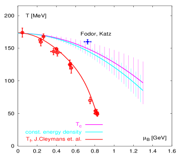
Figure 3: The left hand figure: the statistical model results (broken line) on the energy dependence of $\Lambda/\pi$ ratio. The data are from [21]. The right hand figure: a comparisons of the chemical freeze-out parameters with the phase boundary line. The upper thin line represents the LGT results obtained in Ref. [22] and the lower thin line describes the conditions of constant energy density that was fixed at $\mu=0$ [22]. The full ( Fodor-Katz) point is the end-point of the crossover transition from Ref. [23]. The lower line is the unified freeze-out curve from [20].

One way to partly overcome the above problems in finite density QCD is to use a projection method [3, 10, 16]. Rather than introducing a non–vanishing chemical potential [14], that is formulate QCD in the grand canonical ensemble with respect to U(1)-baryon symmetry, one my go over to a canonical formulation of the thermodynamics and fix directly the baryon number [3, 10, 16]. Following the general discussion of Section 1 the projected partition function onto a given sector of baryon number could be obtained from [3, 16]:

$$Z_{B}(T,V)=\int_{0}^{2\pi}{{d\phi}\over{2\pi}}e^{-iB\phi}Z(\mu_{B}=i\phi,T,V)$$ (23)

where the function $Z$ under the integral represents the grand canonical partition function in Eq.(22) calculated with a complex $\mu_{B}$, and consequently is a real and positive quantity. Nevertheless, due to a Fourier integration the projected partition function still suffers a numerical problem of oscillating functions. However, in the quenched limit of QCD and for moderate values of baryon number the group integration was done analytically and the first results on QCD thermodynamics at finite baryon density were established [16].

The presence of a finite net baryon number modifies non-trivially the properties of QCD medium. As an example of Monte–Carlo study we show in Fig. 2 a heavy quark anti–quark potential obtained from the Polyakov loop correlations [16]. For zero baryon number it shows the usual linearly rising behavior for the quenched case. For finite $B=6$ the potential remains finite at large distances due to screening of the static quark anti–quark pair by the already present net baryon charge in the system.

2.3 Canonical projection in heavy ion collisions

Central heavy ion collisions at relativistic incident energies represent an ideal tool to study nuclear matter at high temperatures and densities. Particle production is – at all incident energies – a key quantity to extract information on the properties of nuclear matter under these extreme conditions. In this context a particular role has been attributed to particles carrying strangeness that is related with U(1) invariance of the strong interactions [2, 6]. The production of secondaries measured in heavy ion collisions was shown in the literature to be very satisfactory described in the context of statistical thermal models [6, 7, 17, 18, 19, 20]. However, already the first attempts to describe strange particle production in low energy central and high energy peripheral heavy ion collisions have shown that the conservation of strangeness should be implemented exactly [6].

An exact formulation of strangeness conservation is implemented through the projection of the partition function onto states of fixed representation of the U(1) group [1]. For the hadron resonance gas the strangeness neutral partition function is obtained from [7]:

$$Z^{C}_{S=0}(T,V)={1\over{2\pi}}\int_{-\pi}^{\pi}d\phi~{}\exp{\left(\sum_{n=-3}^{3}S_{n}e^{in\phi}\right)}$$ (24)

where $S_{n}$ is a thermal phase space available to all particles and resonances that carry strangeness $n$ with $n\in(-3,3)$. The density $n_{s}^{i}$ of particle $i$ carrying strangeness $s$ is derived form (24) as [7]

$$(n_{s}^{i})^{C}=(n_{s}^{i})^{GC}F_{s}(T,V)$$ (25)

where $(n_{s}^{i})^{GC}$ is the grand canonical density and $F_{s}(T,V)$ is the suppression factor that measures a deviation of $(n_{s}^{i})^{C}$ from its asymptotic, grand canonical value. For large $V$ and/or $T$ the factor $F_{s}(T,V)\to 1$. The group projection implies that $F\leq 1$, thus it suppresses a particle densities that carries the U(1) charge. This suppression was found to increase with decreasing collision energy, increasing strangeness content of the particles and decreasing centrality of the collisions [7]. These properties are well observed in experimental data. As an illustration for the model comparison with experimental data [21] we show in Fig. (3–left) the results on the ratio of lambda to pion multiplicities [7].

The statistical model that accounts for an exact conservation of U(1) charges was found in the literature to reproduce the basic features of particle yields obtained in heavy ion and hadron–hadron collisions. The yields were found to be well reproduced with thermal parameters (the temperature and baryon chemical potential) that follow a universal freeze-out line of fixed energy per particle of 1 GeV [20]. The freeze-out line is shown in Fig. (3–right) together with the most recent LGT results on the position of the critical curve in the ($T$–$\mu_{B}$) plane [22, 23].

Acknowledgements: We wish to thank P. Braun-Munzinger and L. Turko for interesting discussions. K.R acknowledges the support of the Alexander von Humboldt Foundation.

References

- [1] K. Redlich and L. Turko, Z. Phys. B97 (1980) 279; L. Turko, Phys. Lett. B104 (1981).
- [2] 153; R. Hagedorn and K. Redlich, Z. Phys. C27 (1985) 541; Rafelski and M. Danos, Phys. Lett. B97 (1980) 279; L. Turko and J. Rafelski, Eur. Phys. J. C18 (2001) 587.
- [3] D. Miller and K. Redlich, Phys. Rev. D37 (1988) 3716; Phys. Rev. D35 (1987) 2524; H. Th. Elze, D. Miller and K. Redlich, Phys. Rev. D35 (1987) 748.
- [4] D.H. Rischke, M.I. Gorenstein, A. Schäfer, H. Stöcker and W. Greiner, Phys. Let. B278 (1992) 19; Z. Phys. C56 (1992) 325.
- [5] A.B. Balantekin, Phys. Rev. E64 (2001) 066105; P.N. Meisinger, et al., Phys. Rev. D65 (2002) 034009; M.I. Gorenstein, et al., Phys. Let. B524 (2002) 265; H. Th. Elze, et. al., Phys. Let. B506 (2001) 123; A.G. Michael, et. al., Phys. Rev. D59 (1999) 034009; M.G. Mustafa, et al., Euro Phys. J. C5 (1988) 711; C.D. Fosco, Phys. Rev. D57 (1988) 6554; C. Spieles, et. al., Phys. Rev. C57 (1998) 908; L.D. Mc Lerran and A. Sen, Phys. Rev. D32 (1985) 2794.
- [6] P. Braun-Munzinger, et al., Nucl. Phys. A697 (2002) 902 and references therein.
- [7] A. Tounsi, et al., J. Phys G28 (2002) 2095; Eur. Phys. J. C24 (2002) 35; J. S. Hamieh, K. Redlich, and A. Tounsi, Phys. Lett. B486 (2000) 61
- [8] C.M. Ko, et al., Phys. Rev. Lett. 86 (2001) 5438; S. Jeon, et al., Nuc. Phys. A697 (2002) 546.
- [9] J. Engels, et al., Z. Phys. C42 (1989) 341; A. Peshier, et al., Phys. Rev. C61 (2000) 045203.
- [10] A. Roberge and N. Weiss, Nucl. Phys. B275 [FS17] (1986) 734.
- [11] A. Gocksch, R.D. Pisarski, Nucl. Phys. B402 (1993) 657; R. Pisarki, hep-ph/0203271; Nucl. Phys. A702 (2002) 151; A. Dumitru and R. Pisarski, Phys. Lett. B525 (2002) 95.
- [12] For a recent review see: I.M. Barbour, S.E. Morrison, E.G. Klepfish, J.B. Kogut and M.P. Lombardo, Nucl. Phys. B (proc. Suppl.) 60 (1998) 220.
- [13] F. Karsch, Lect. Notes. Phys. 583 (2002) 209; I. Barbour, et al., Nucl. Phys. Proc. Supp. 60A (1998) 220.
- [14] P. Hasenfratz and F. Karsch, Phys. Lett. B125 (1983); J. Kogut et al., Nucl. Phys. B225 [FS9] (1983) 93.
- [15] B. Berg, J. Engels, E. Kehl, B. Waltl and H. Satz, Z. Phys. C31 (1986) 167.
- [16] F. Karsch, Nucl. Phys. Proc. Suppl. 83 (2000) 14; J. Engels et al., Nucl. Phys. Proc. Suppl. 83 (2000) 366; Nucl. Phys. B558 (1999) 307; O. Kaczmarek et al., Phys. Rev. D62 (2000) 034021.
- [17] P. Braun-Munzinger, I. Heppe, and J. Stachel, Phys. Lett. B465 (1999) 15; P. Braun-Munzinger and J. Stachel, J. Phys. G28 (2002) 1971; Phys. Lett. B490 (2000)196; Nucl. Phys. A690 (2001) 119c; A. Keränen, and F. Becatini, J. Phys. G28 (2002) 2041; Becattini, et al., Phys. Rev. C64 (2001) 024901.
- [18] J. Letessier, and J. Rafelski, Int. J. Mod. Phys. E9 (2000) 107.
- [19] P. Braun-Munzinger, et al., Phys. Lett. B518 (2001) 41; D. Magestro, J. Phys. G28 (2002) 1745.
- [20] J. Cleymans, et al., Phys. Rev. C60 (1999) 0544908; Phys. Rev. Lett. 81 (1998) 5284; Phys. Rev. C59 (1999) 1663; Phys. Lett. B485 (2001) 27.
- [21] A. Mischke, for NA49 Collaboration, nucl-ex/0209002.
- [22] S. Ejiri, et al., hep-lat/0209012; C. Schmidt, et al., hep-lat/0209009.
- [23] Z. Fodor and S.D. Katz, Phys. Lett. B534 (2002) 87.