Abstract

The first results from the KamLAND experiment in conjunction with the global solar neutrino data has demonstrated striking ability to constrain the $\Delta m^{2}_{\odot}$ ($\Delta m^{2}_{21}$) very precisely. However the allowed range of $\theta_{\odot}$ ($\theta_{12}$) did not change much with the inclusion of the KamLAND results. In this paper we probe if future data from KamLAND can increase the accuracy of the allowed range in $\theta_{\odot}$ and conclude that even after 3 kton-year of statistics and most optimistic error estimates, KamLAND may find it hard to significantly improve the bounds on the mixing angle obtained from the solar neutrino data. We discuss the $\theta_{12}$ sensitivity of the survival probabilities in matter (vacuum) as is relevant for the solar (KamLAND) experiments. We find that the presence of matter effects in the survival probabilities for ${}^{8}B$ neutrinos give the solar neutrino experiments SK and SNO an edge over KamLAND, as far as $\theta_{12}$ sensitivity is concerned, particularly near maximal mixing. Among solar neutrino experiments we identify SNO as the most promising candidate for constraining $\theta_{12}$ and make a projected sensitivity test for the mixing angle by reducing the error in the neutral current measurement at SNO. Finally we argue that the most accurate bounds on $\theta_{12}$ can be achieved in a reactor experiment, if the corresponding baseline and energy can be tuned to a minimum in the survival probability. We propose a new reactor experiment which can give the value of $\tan^{2}\theta_{12}$ to within 14%. We also discuss the future Borexino and LowNu experiments.

1 Introduction

The year 2002 has witnessed two very important results in solar neutrino research. In April 2002 the accumulated evidence in favor of possible flavor conversion of the solar electron neutrinos was confirmed with a statistical significance of 5.3$\sigma$ from the Sudbury Neutrino Observatory (SNO) [1]. The inclusion of the SNO spectrum data combining the charged current, electron scattering and neutral current events in the global solar neutrino analysis picked out the Large Mixing Angle (LMA) MSW [2] solution as the preferred solution [3, 4], confirming the earlier trend [5]. In December 2002 the Kamioka Liquid scintillator Anti-Neutrino Detector (KamLAND) experiment in Japan [6] provided independent and conclusive evidence in favor of the LMA solution, using reactor neutrinos. Assuming CPT invariance this establishes oscillations of $\nu_{e}$ with a mass squared difference $\sim 7\times 10^{-5}$ eV² and large mixing [7, 8]. Comprehensive evidence in favor of oscillation of the atmospheric $\nu_{\mu}$s came from the Super-Kamiokande (SK) results [9]. This was confirmed by the result from the K2K long baseline experiment using terrestrial neutrino sources [10]. The best-fit value of $\Delta m^{2}_{atm}$ comes out as $\sim 2.5\times 10^{-3}$ eV² with maximal mixing in the ${\nu_{\mu}}-{\nu_{\tau}}$ sector [11].

Since the solar and atmospheric neutrino anomalies involve two hierarchically different mass scales, simultaneous explanation of these involve three neutrino mixing. There are nine unknown parameters involved in the three-generation light neutrino mass matrix – masses of the three neutrinos, and six other parameters coming from the Pontecorvo-Maki-Nakagawa-Sakata (PMNS) mixing matrix [12]. Of the nine parameters, oscillation experiments are sensitive to six ($\Delta m^{2}_{21}$, $\Delta m^{2}_{31}$, $\theta_{12}$, $\theta_{13}$, $\theta_{23}$, $\delta$), the two independent mass squared differences ($\Delta m_{ij}^{2}=m_{i}^{2}-m_{j}^{2}$), the three mixing angles and one CP phase. Flavor oscillations are independent of the absolute neutrino mass scale, and the remaining two CP phases appear only in lepton number violating processes. The solar neutrino data constrain the parameters $\Delta m^{2}_{\odot}\sim\Delta m^{2}_{21}$ and $\theta_{\odot}\sim\theta_{12}$ while the atmospheric neutrino data constrain the parameters $\Delta m^{2}_{atm}\sim\Delta m_{31}^{2}$ and $\theta_{atm}\sim\theta_{23}$. The two sectors get connected by the mixing angle $\theta_{13}$ which is at present constrained by the reactor data [13, 14] as $\sin^{2}\theta_{13}\leq 0.03$ at 90% C.L. [13].

With neutrino flavor oscillations in both solar and atmospheric neutrino anomalies confirmed, the research in neutrino physics is now all set to enter the era of precision measurements. The conventional accelerator based long baseline experiments as well as neutrino factories using muon storage rings as sources have been discussed widely for the purposes of precise determination of the neutrino oscillation parameters (see [15] for a comprehensive discussion and a complete list of references). The major goals in the upcoming long baseline and proposed neutrino factories are – precision determination of $|\Delta m^{2}_{31}|$ and $\theta_{23}$ , ascertaining the sign of $\Delta m^{2}_{31}$ and determining how small is $\theta_{13}$. The atmospheric parameters $|\Delta m_{31}^{2}|$ and $\sin^{2}2\theta_{23}$ are expected to be determined within 1% accuracy in the next generation long baseline experiments using conventional (super)beams [16, 17]. The mixing angle $\sin^{2}2\theta_{13}$ is expected to be probed down to $1.5\times 10^{-3}$ in the long baseline experiments using superbeams [16, 17] while neutrino factories will be sensitive upto $\sin^{2}2\theta_{13}\sim 10^{-5}$ [15]. Finally with KamLAND confirming the LMA solution, it should be possible to measure the CP phase $\delta$ in neutrino factories and possibly even in the proposed phase II JHF (in Japan) and NuMI (in USA) long baseline experiments, provided $\sin^{2}2\theta_{13}$ is not too small [16, 17]. However $\Delta m^{2}_{21}$ and $\theta_{12}$ drive the sub-leading oscillations in these experiments and hence precision determination of these parameters through long baseline experiments or neutrino factories will be very challenging. Therefore in all these studies the sub-leading oscillation parameters $\Delta m^{2}_{21}$ and $\theta_{12}$ are introduced as external inputs, taking typically either the best-fit value obtained from the global solar analysis or the projected sensitivity limits from future KamLAND data. However, since the concern now has shifted to precision measurements, the uncertainty in the parameters $\Delta m^{2}_{21}$ and $\theta_{12}$ can also affect the accuracy with which we can determine the rest of the parameters of the PMNS matrix, especially the CP violation parameter $\delta$, as it comes only with the sub-leading term in the oscillation probability. The uncertainty in the measurement of other parameters, introduced through the uncertainty in the solar parameters, gets worse for smaller values of the mixing angle $\sin^{2}2\theta_{13}$.

As far as the precision determination of $\Delta m^{2}_{21}$ is concerned, KamLAND has already demonstrated an extraordinary capability in precisely determining the $\Delta m^{2}_{\odot}$. The uncertainty (we call it “spread”) in the 99% C.L. allowed range of this parameter around the global best-fit solution (which we call the low-LMA), has reduced to 30% after including the KamLAND spectral data, from 76% as obtained from only solar global analysis. The spread in the allowed range of $\tan^{2}\theta_{\odot}$ on the other hand remains unchanged, even after including the KamLAND results and the current 99% C.L. uncertainty is $\sim$ 47%.

In this paper we probe the sensitivity of the various previous, present and future solar neutrino experiments to the parameter $\theta_{\odot}\sim\theta_{12}$ and make a comparative study of which experiment is most sensitive in constraining $\theta_{12}$. We conclude that SNO has the best potential for constraining $\theta_{12}$ . We make an optimistic projected analysis including future SNO neutral current (NC) measurements and look for the improved bounds on $\theta_{12}$ . We discuss the precipitating factors for which the sensitivity of KamLAND to $\theta_{12}$ is not as good as its sensitivity to $\Delta m^{2}_{21}$ and discuss the effect of increased statistics and reduced systematics through projected analyses. We conclude that even with 3 kTy statistics KamLAND may not significantly improve the current limits on $\theta_{12}$ coming from the solar neutrino experiments. We differentiate between two types of terrestrial experimental set-ups sensitive to vacuum oscillations. One which has its energy and baseline tuned to a maximum in the survival probability and another where the baseline ($L$) and energy ($E$) would give a minimum in the survival probability. We argue that sensitivity to $\theta_{12}$ increases substantially if the experiment is sensitive to a “Survival Probability MINimum” (SPMIN) instead of a “Survival Probability MAXimum” (SPMAX) – as is the case in KamLAND, and propose a new reactor experiment which would give precise value of $\tan^{2}\mbox{$\theta_{12}$~{}}$ down to 14%.

We begin in Section 2 with a discussion of the potential of the experiments sensitive to different limits of the survival probability in constraining the mixing angle. We then discuss the solar neutrino experiments and delineate the impact of each one separately on the global allowed areas. We obtain bounds on $\theta_{12}$ from a future SNO NC data. In the next section we introduce the KamLAND data and discuss how much the uncertainty in $\theta_{12}$ is going to reduce with the increased statistics in KamLAND. We make a comparative study of various solar neutrino experiments along with KamLAND data and determine the role of the individual experiments in constraining $\theta_{12}$ and $\Delta m^{2}_{21}$. The reasons for the low sensitivity of KamLAND to $\theta_{12}$ is expounded. In Section 4 we propose a new reactor experiment which could in principle bring down the uncertainty in $\tan^{2}\mbox{$\theta_{12}$~{}}$ to 14%. In the next section we examine the role of the future solar neutrino experiments – Borexino and the LowNu experiments. We finally present our conclusions in Section 6.

2 Solar Neutrino Experiments

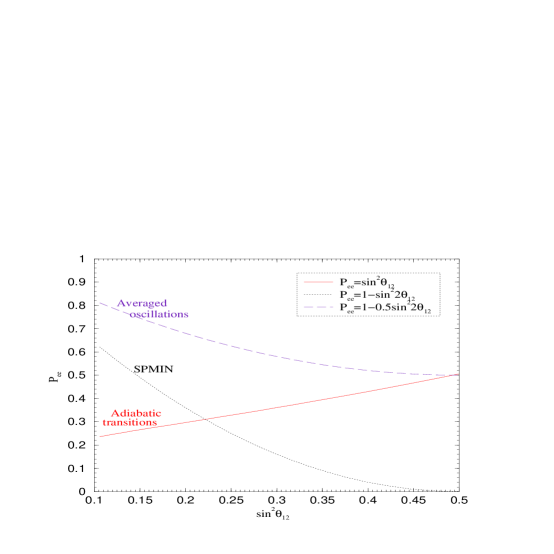
Figure 1: The survival probability $P_{ee}$ as a function $\sin^{2}\theta_{12}$ for $P_{ee}=\sin^{2}\theta_{12}$ (solid line), $P_{ee}=1-0.5\sin^{2}2\theta_{12}$ (dashed line) and $P_{ee}=1-\sin^{2}2\theta_{12}$ (dotted line).

The solar neutrinos come with a wide energy spectrum and have been observed on Earth in detectors with different energy thresholds. The survival probability for the low energy $pp$ (in Ga experiments – SAGE, GALLEX and GNO) and the high energy ${}^{8}{B}~{}$fluxes (in SK and SNO) in the now established LMA scenario can be very well approximated by

$$P_{ee}({pp})\approx 1-\frac{1}{2}\sin^{2}2\mbox{$\theta_{12}$~{}}$$ (1)

$$P_{ee}({\mbox{${}^{8}{B}~{}$}})\approx\sin^{2}\mbox{$\theta_{12}$~{}}+f_{reg}$$ (2)

where $f_{reg}$ is the ${\nu_{e}}$ regeneration inside the Earth. Thus the solar neutrinos in LMA are sensitive to $\theta_{12}$ , the degree of sensitivity depending on the energy of the relevant solar neutrinos observed. To expound this feature we present in Figure 1 the variation of $P_{ee}$ with $\sin^{2}\mbox{$\theta_{12}$~{}}$ for the different limits of the neutrino oscillation scenarios – averaged oscillations (cf. Eq.(1)), fully adiabatic conversions in matter (cf. Eq(2)) and “full” vacuum oscillations corresponding to “Survival Probability MINimum” (SPMIN), that is $P_{ee}=1-\sin^{2}2\mbox{$\theta_{12}$~{}}$. For both averaged oscillations and SPMIN the dependence of the probability is quadratic in $\sin^{2}\mbox{$\theta_{12}$~{}}$, while for complete adiabatic conversions (AD) the dependence is linear. Thus for the latter the error in $\sin^{2}\mbox{$\theta_{12}$~{}}$ is roughly same as the error in the probability $P_{ee}$.

$$(\Delta\sin^{2}\mbox{$\theta_{12}$~{}})_{\rm AD}\sim\Delta P_{ee}$$ (3)

While the corresponding error for averaged oscillations (AV) and SPMIN cases are roughly given by

$$(\Delta\sin^{2}\mbox{$\theta_{12}$~{}})_{\rm AV}\sim\frac{\Delta P_{ee}}{-2\cos 2\mbox{$\theta_{12}$~{}}}$$ (4)

$$(\Delta\sin^{2}\mbox{$\theta_{12}$~{}})_{\rm SPMIN}\sim\frac{\Delta P_{ee}}{-4\cos 2\mbox{$\theta_{12}$~{}}}$$ (5)

the sensitivity to $\sin^{2}\mbox{$\theta_{12}$~{}}$ for averaged oscillations being reduced to roughly 1/2 of that for SPMIN. We note from Eqs.(3), (4) and (5) that for mixing angle not very close to maximal mixing, that is for $\cos 2\mbox{$\theta_{12}$~{}}\>\raisebox{-2.15277pt}{$\stackrel{{\scriptstyle\textstyle>}}{{\sim}}$}\>0.25$ ($\sin^{2}\mbox{$\theta_{12}$~{}}\>\raisebox{-2.15277pt}{$\stackrel{{\scriptstyle\textstyle<}}{{\sim}}$}\>0.375$), the error in $\theta_{12}$ is least when we have a SPMIN. For $\cos 2\mbox{$\theta_{12}$~{}}\>\raisebox{-2.15277pt}{$\stackrel{{\scriptstyle\textstyle>}}{{\sim}}$}\>0.5$ ($\sin^{2}\mbox{$\theta_{12}$~{}}\>\raisebox{-2.15277pt}{$\stackrel{{\scriptstyle\textstyle<}}{{\sim}}$}\>0.25$) even averaged oscillations are better suited for $\theta_{12}$ measurements than adiabatic conversions inside matter. However for large mixing angles close to maximal, the adiabatic case has the maximum sensitivity. All these features are evident in the Figure 1 which shows that for the SPMIN case and for mixing not too close to maximal, the $P_{ee}$ has the sharpest dependence on the mixing angle and the $\theta_{12}$ sensitivity is maximum. Since the 99% C.L. allowed values of $\theta_{12}$ is within the range $0.14<\cos 2\mbox{$\theta_{12}$~{}}<0.57$, SPMIN seems most promising for constraining $\theta_{12}$.

2.1 Bounds from current solar data

While the Gallium (Ga) experiments, SAGE, GALLEX and GNO [19] are sensitive mostly to the $pp$ neutrinos, the SK [20] and SNO [1] predominantly observe the higher energy ${}^{8}{B}~{}$neutrino flux. The Chlorine experiment (Cl) [21] observes the intermediate energy ${}^{7}{Be}$ neutrinos in addition to the ${}^{8}{B}~{}$. Since the best-fit value for the mixing angle is large (with $\sin^{2}\theta_{12}\approx 0.3$), from the discussion above we expect SK and SNO to have a better handle over $\theta_{12}$. However the observed rates in the detectors depend not only on the survival probability but also on the initial solar neutrino flux in the Sun. The errors in the predicted fluxes are carried over to the errors in the parameters determined, reducing the net sensitivity. While the $pp$ neutrinos are very accurately predicted and have theory errors of less than $\sim 1\%$, the ${}^{8}{B}~{}$neutrinos have a huge Standard Solar Model (SSM) uncertainty of $\sim 20\%$ [22]. Thus on this front the “sub-MeV” experiments score over the higher energy solar neutrino experiments.

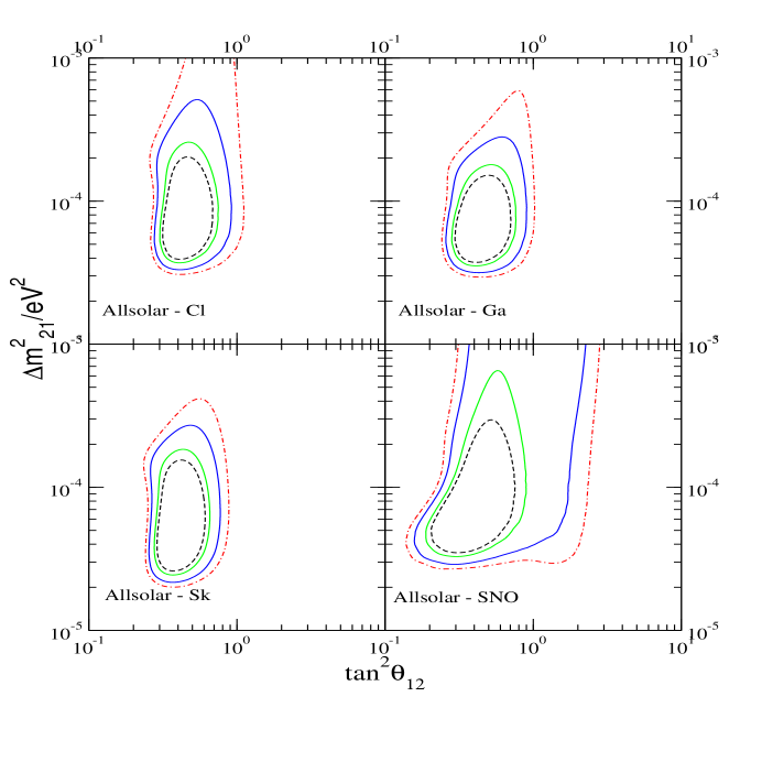
Figure 2: The 90%, 95%, 99% and 99.73% C.L. contours from a $\chi^{2}$ analysis using all but one of the solar neutrino experiments. The experiment left out from analysis is indicated in the panels.

SK and SNO are real-time experiments and hence carry information regarding energy dependence of the suppression and potential matter effects as well. To project a realistic scenario of the potential of each of the solar neutrino experiments in constraining the parameters, we present in Figure 2 the C.L. allowed contours from an analysis where all but one of the experiments is not considered. The figure shows that exclusion of Cl from the analysis raises the upper limit on both $\Delta m_{21}^{2}$ and $\theta_{12}$ . Higher values of $\Delta m_{21}^{2}$ and values of $\theta_{12}$ close to maximal mixing give an energy independent suppression of the solar neutrino flux within $\pm 10\%$ [24]. The Cl experiment with an observed rate that is $2\sigma$ away from that predicted by maximal mixing disfavors these zones. So omission of Cl makes these zones more allowed. SK is consistent with no energy dependence in the survival probability. Thus SK favors these quasi-energy independent regions of the parameter space. The non-observation of any significant day-night asymmetry in SK puts the lower bound on $\Delta m^{2}_{21}$ and hence omission of SK loosens this bound. The Ga observed rate of 0.55 is comparatively closer to the rate predicted at maximal mixing ($=0.5$), however the error in the $pp$ flux is only $\sim 1\%$ and this helps Ga to disfavor maximal mixing. Therefore excluding Ga slightly increases the upper limit of $\theta_{12}$ . But the strongest impact on the allowed regions of the parameter space comes from SNO, which comprehensively rules out most of these quasi-energy independent zones that predict a suppression rate $P_{ee}\>\raisebox{-2.15277pt}{$\stackrel{{\scriptstyle\textstyle>}}{{\sim}}$}\>0.5$. Thus without SNO the bounds become much weaker in both $\Delta m_{21}^{2}$ and $\theta_{12}$ . The upper limit on $\Delta m_{21}^{2}$ vanishes and the upper limit on $\theta_{12}$ becomes extremely poor, with large areas in the “dark zone” (zones with $\mbox{$\theta_{12}$~{}}>\pi/4$) getting allowed. Without SNO these areas were allowed since the 20% uncertainty in the ${}^{8}{B}~{}$neutrino flux could be used to compensate for the higher survival probability and explain the global data. However with SNO the uncertainty in ${}^{8}{B}~{}$flux has come down to 12%, putting a sharp upper bound to both $\Delta m_{21}^{2}$ ($\mbox{$\Delta m_{21}^{2}$~{}}<2.2\times 10^{-4}$ eV²) and $\theta_{12}$ ($\tan^{2}\mbox{$\theta_{12}$~{}}<0.77$) at 99% C.L..

2.2 Sensitivity of expected NC data from SNO

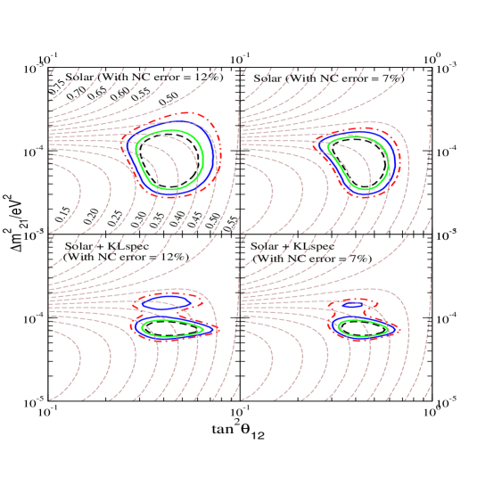
Figure 3: The impact of the future SNO NC data (with error of 7%) on the parameter space. The upper panels are for the global solar neutrino data with current (12%) and future (7%) error in NC. The lower 2 panels are the corresponding allowed regions obtained by combining the KamLAND and the solar neutrino data. The lines of constant CC/NC ratio in SNO are shown by dashed lines.

This tremendous power of SNO to constrain mass and mixing parameters stems from its ability to simultaneously measure the neutrino suppression rate through the charged current (CC) interaction and the total ${}^{8}{B}~{}$neutrino flux through the independent neutral current (NC) measurement. Thus by reducing errors in both $P_{ee}$ (from CC reaction) and the ${}^{8}{B}~{}$flux normalization $f_{B}$ (from the NC reaction), SNO can put better limits on the mass and mixing parameters. In particular it bounds the LMA zone in $\Delta m_{21}^{2}$ from the top, chopping off parts of the parameter space for which the ${}^{8}{B}~{}$neutrinos do not undergo resonant transitions inside the Sun and therefore have a form of $P_{ee}\approx 1-0.5\sin^{2}2\mbox{$\theta_{12}$~{}}$. These regions would give a $P_{ee}>0.5$ and could be accommodated with the CC data only if the initial ${}^{8}{B}~{}$flux was assumed to be less, or in other words $f_{B}<1$. However values of $f_{B}$ different from 1 are disfavored from the NC measurements of SNO and these high $\Delta m_{21}^{2}$ regions get ruled out. Similarly in the adiabatic zone since $P_{ee}\approx\sin^{2}\mbox{$\theta_{12}$~{}}$, the larger values of $\sin^{2}\mbox{$\theta_{12}$~{}}$ close to maximal mixing would be allowed only if $f_{B}$ were to be assumed to be less than 1, which is at variance with the data as discussed above and hence these zones get severely constrained.

The upper left-hand panel of Figure 3 shows the current C.L. allowed zones from the global solar neutrino experiments. Superimposed on them are the lines of constant CC/NC rates in SNO. We note that the $3\sigma$ range of predicted CC/NC rates from the current solar limits are $0.23-0.47$. If SNO can measure a CC/NC ratio with smaller errors then the range for the allowed values of $\theta_{12}$ would reduce.

The next phase of NC rate from SNO would come from capture of the neutron – released in the neutral current breakup of heavy water – on ${}^{35}Cl$ (salt). This data is expected to have much better statistics than the earlier data released last year, which was with neutron capture on deuterons. Since the efficiency of neutron captures on salt is about 83% while that on deuterons only about 30% we expect the statistical errors in the neutral current measurements to come down to about 5%. It would be interesting to gauge how much the uncertainty in $\theta_{12}$ would reduce with better measurements of the total ${}^{8}{B}~{}$flux from SNO. Just to project the impact of reduced errors from SNO we show in the upper right-hand panel of Figure 3 the allowed areas in the parameter space when the total error in the NC measurement is reduced to 7%. Since the purpose of this figure is not accuracy but an optimistic projection of the impact of a futuristic SNO NC measurement, we have replaced the 34-binned SNO spectrum data used everywhere else in this paper, with the total charged and neutral current rates in SNO. The total rates are disentangled from the SNO spectrum data by assuming no spectral distortion for the ${}^{8}{B}~{}$flux. Since we confine ourselves to the LMA zone where there is hardly any spectral distortion expected, we consider this to be an excellent approximation. We note that the limit on $\theta_{12}$ improves with reduced errors in NC and the 99% C.L. bounds at $\mbox{$\Delta m_{21}^{2}$~{}}=7\times 10^{-5}$ eV² reads $0.3<\tan^{2}\mbox{$\theta_{12}$~{}}<0.63$.

3 KamLAND

3.1 Current Bounds

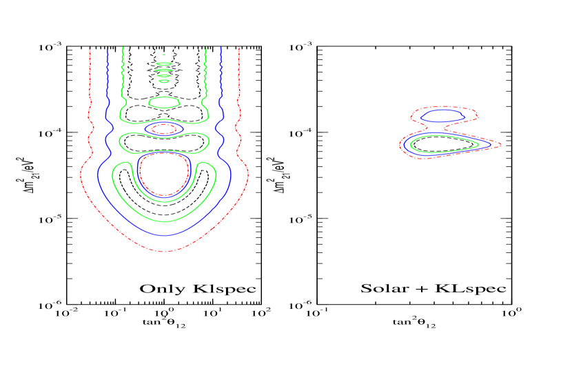
Figure 4: The 90%, 95%, 99% and 99.73% C.L. contours from a $\chi^{2}$ analysis using the KamLAND spectrum data alone (left panel) and the combined KamLAND and global solar data (right panel).

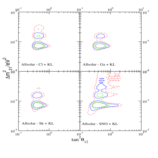
Figure 5: Same as Figure 2 but with the KamLAND data included.

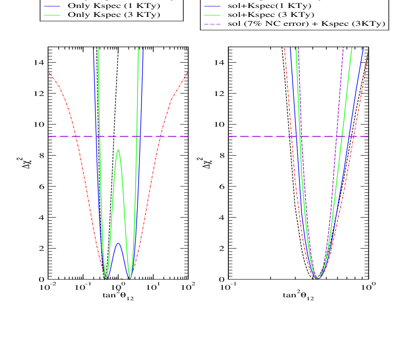
Figure 6: $\Delta\chi^{2}$ versus $\tan^{2}\mbox{$\theta_{12}$~{}}$ for only KamLAND data (left panel) and combined KamLAND and Solar neutrino data (right panel). For KamLAND we use the declared 0.162 kTy data as well as the 1 kTy and 3 kTy projected spectral data, with the spectrum simulated at the low-LMA best-fit point. The long-dashed line gives the 99% C.L. bound for 2 parameter fit.

After the announcement of the first KamLAND results [6] there was a plethora of papers discussing the impact of KamLAND on the mass and mixing parameters, $\Delta m_{\odot}^{2}$ and $\theta_{\odot}$ [7, 8]. The KamLAND spectrum even though still short on statistics, is powerful enough to disintegrate the solar neutrino parameter space into two disjoint islands at the 99% C.L. – one around the global best-fit of $\mbox{$\Delta m_{21}^{2}$~{}}=7.17\times 10^{-5}$ eV² and $\tan^{2}\theta_{12}=0.44$ and another at $\mbox{$\Delta m_{21}^{2}$~{}}=1.49\times 10^{-4}$ eV² and $\tan^{2}\theta_{12}=0.43$. We call them low-LMA and high-LMA respectively. High-LMA appears at a reduced statistical significance of about $2\sigma$. The two islands however join at the $3\sigma$ level. We show the currently allowed zones in Figure 4. The right-hand panel of this figure gives the allowed areas from the KamLAND data alone, while the left-hand panel gives the combined allowed zones from solar and KamLAND data. From a global analysis involving the solar and KamLAND data the $3\sigma$ ranges are

$$0.27 <~{}\tan^{2}\theta_{12}~{}< 0.88$$ (6)

$$4.96\times 10^{-5} <~{}\Delta m_{21}^{2}~{}< 2.0\times 10^{-4}$$ (7)

The 99% range for the parameters are [7],

$$0.28 <~{}\tan^{2}\theta_{12}~{}< 0.79$$ (8)

$$5.3\times 10^{-5} <~{}\Delta m_{21}^{2}~{}< 9.9\times 10^{-5},~{}~{}~{}({\rm low-LMA})$$ (9)

$$0.34 <~{}\tan^{2}\theta_{12}~{}< 0.55$$ (10)

$$1.3\times 10^{-4} <~{}\Delta m_{21}^{2}~{}< 1.8\times 10^{-4},~{}~{}~{}({\rm high-LMA})$$ (11)

We note that low-LMA allows a much larger range of $\theta_{12}$ than high-LMA. This has more to do with the fact that the global best-fit is in low-LMA than anything else. If the contour at high-LMA was to be plotted with respect to the local minima at high-LMA, then the allowed range of $\theta_{12}$ would be almost the same.

To study the impact of each of the solar neutrino experiments in determining the allowed range of the mixing parameters in conjunction with KamLAND, we show in Figure 5 the allowed areas from a combined analysis involving the KamLAND data and the solar data, with each panel showing the areas obtained when one of the solar neutrino experiments is excluded. The Figure shows that neglecting Cl helps to make the high-LMA slightly more allowed and the 3$\sigma$ contour extends to larger $\Delta m^{2}$ while omission of Ga and SK does not change the contours much with respect to the global contours of figure. 4. However the exclusion of SNO completely removes the upper bound on $\Delta m_{21}^{2}$ and allows $\theta_{12}$ to move into the “dark zone” even at 99% C.L.. This again exemplifies the power of SNO in constraining the quasi-energy independent zones as discussed in the previous section. In fact we have checked that SNO alone combined with KamLAND, can almost restrict both $\Delta m_{21}^{2}$ and $\theta_{12}$ within the current global allowed range.

3.2 Reduced SNO NC errors and KamLAND 

It would be interesting to check if the KamLAND data with future solar neutrino data in general and SNO NC data in particular, could improve the limits on the parameters or not. The lower 2 panels in Figure 3 show the impact of the next phase SNO NC data in conjunction with the KamLAND data. The lower left panel of the figure shows the current global allowed regions obtained from the combined solar and KamLAND data. Also shown superimposed are the constant lines for the CC/NC rates in SNO. The predicted $3\sigma$ range for the CC/NC rates is seen to be $0.27-0.47$. The lower right hand panel gives the allowed areas obtained when the error in NC measurement is reduced from 12% to 7% as discussed earlier. We again reiterate that for this figure with future SNO NC measurement we have used the CC and NC rates instead of the full SNO day-night spectrum used in the rest of the paper. The combination of the solar with reduced NC errors and KamLAND is seen to constrain $\theta_{12}$ to $0.3<\tan^{2}\mbox{$\theta_{12}$~{}}<0.63$ at 99% C.L., which is the same as that obtained without KamLAND and with improved NC. Thus we again note that inclusion of the current KamLAND data in the global analysis brings no improvement on the limits for $\theta_{12}$ . The results obtained from a combined future SNO NC and future KamLAND data are presented in the following sections.

3.3 Sensitivity of projected KamLAND data

In [7] we made a projected analysis using the 1 kTy KamLAND spectrum simulated at some strategic points in and around the high-LMA and low-LMA allowed regions and probed the potential of a statistics enriched KamLAND data sample to plump for the right solution between the two. The 3 kTy KamLAND data is obviously expected to further tighten the bounds on the mixing parameters [26]. The sensitivity of KamLAND to $\Delta m_{21}^{2}$ is found to be remarkable. To study the limits that KamLAND would be expected to impose on the mixing angle $\theta_{12}$ with more statistics, we present in Figure 6 the $\Delta\chi^{2}(=\chi^{2}-\chi^{2}_{min})$ as a function of $\tan^{2}\mbox{$\theta_{12}$~{}}$, keeping $\Delta m_{21}^{2}$ free. The left-hand panel gives the limits obtained from KamLAND data alone, with the declared 0.162 kTy data and the projected 1 kTy and 3 kTy data, simulated at the current low-LMA best-fit point. The right-hand panel gives the corresponding bounds when KamLAND is combined with the solar data. The limits on the value of $\theta_{12}$ will depend somewhat on the point in the parameter space where the projected KamLAND spectra are simulated. We present here just the bounds obtained if the future KamLAND spectrum sticks to its current trend and roots for the low-LMA best-fit point. Also shown in both the panels is the curve corresponding to the global solar neutrino data alone.

Apart from the increased statistics we have also studied the role of the reduced systematics on the allowed parameter ranges. The current 0.162 kTy KamLAND data has a rather large and very conservative systematic error of 6.42% [6]. However the KamLAND collaboration hopes to improve their systematics in the future. The bulk of the systematic error comes from the error in the knowledge of the fiducial volume which could be improved by making calibration measurements. For 1 kTy data the systematic error could reduce to the 5% level with better understanding of the detector and more statistics. For the 3 kTy data sample the systematic uncertainties could be lowered to even 3% with three-dimensional calibrations and better understanding of reactor neutrino flux. We have assumed an expected 5% systematic uncertainty for our analysis with the 1 kTy KamLAND data and a more optimistic 3% systematic uncertainty for the 3 kTy data sample.

From the Figure 6 we see that even with 3 kTy statistics (and with only 3% systematic error), KamLAND would constrain $\theta_{12}$ only marginally better than the current solar neutrino experiments. Also, KamLAND being insensitive to matter effects has a $\theta_{12}$  and $\pi/2-\mbox{$\theta_{12}$~{}}$ ambiguity and therefore allows regions on both side of maximal mixing. Maximal mixing itself cannot be ruled out by the 3 kTy KamLAND data alone. The right-hand panel shows that the combined $\theta_{12}$ limits from the global solar neutrino data and future KamLAND data, would be somewhat more constricted than that obtained from the current solar data alone. Also shown in the right-hand panel of Figure 6 is the $\theta_{12}$ sensitivity curve obtained by combining the 3 kTy KamLAND data (with 3% systematic uncertainty) with the global solar neutrino data, where the total uncertainty in the SNO NC data has been reduced from 12% as of now, to only 7% expected from a future SNO measurement. Reduction of the SNO NC error reduces the combined allowed $\theta_{12}$ range as discussed in Section 3.2, particularly on the large mixing side.

Data	99% CL	99% CL	1 $\sigma$	2$\sigma$	99% CL	1 $\sigma$	2 $\sigma$	99% CL
set	range of	spread	range	range	range	spread	spread	spread
used	$\mbox{$\Delta m_{21}^{2}$~{}}\times$	of	of	of	of	in	in	in
	10-5eV2	$\Delta m_{21}^{2}$	$\tan^{2}\theta_{12}$	$\tan^{2}\theta_{12}$	$\tan^{2}\theta_{12}$	$\tan^{2}\theta_{12}$	$\tan^{2}\theta_{12}$	$\tan^{2}\theta_{12}$
only sol	3.2 - 24.0	76%	$.33-.53$	$.29-.66$	$.27-.75$	23%	39%	47%
sol+162 Ty	5.3 - 9.9	30%	$.34-.55$	$.30-.68$	$.28-.78$	23%	39%	47%
sol+1 kTy	6.7 - 8.0	9%	$.36-.54$	$.33-.65$	$.30-.72$	20%	33%	41%
sol+3 kTy	6.8 - 7.7	6%	$.37-.52$	$.34-.59$	$.33-.65$	17%	27%	33%
sol(7%)+3 kTy	6.8 - 7.7	6%	$.38-.50$	$.35-.56$	$.33-.60$	14%	23%	29%

Table 1: The range of parameter values allowed and the corresponding spread. For the current observed solar+KamLAND analysis we show the ranges and the spread only in the low-LMA region. For the 1 kTy and 3 kTy ranges we have simulated the spectrum at the current low-LMA best-fit. We assume 5% systematic error for 1 kTy KamLAND spectrum and 3% systematic error for 3 kTy KamLAND spectrum. The last row of the Table corresponds to a combination of the 3 kTy KamLAND data and the global solar neutrino data where the SNO NC error has been reduced to only 7%.

In Table 1 we explicitly present the 99% C.L. allowed ranges for the solar neutrino parameters in low-LMA, allowed from combined solar and KamLAND. Shown are the current bounds on $\Delta m_{21}^{2}$ and $\tan^{2}\mbox{$\theta_{12}$~{}}$ and those expected after 1 kTy and 3 kTy of KamLAND data taking. The sensitivity of KamLAND to $\Delta m_{21}^{2}$ is tremendous. Since the thrust of this paper is to study the limits on the solar mixing angle, we also give the $1\sigma$ and $2\sigma$ limits for $\tan^{2}\mbox{$\theta_{12}$~{}}$. Also shown are the % spread in the oscillation parameters. We define the “spread” as

$${\rm spread}=\frac{prm_{max}-prm_{min}}{prm_{max}+prm_{min}}\times 100$$ (12)

where ${prm}$ denotes the parameter $\Delta m_{21}^{2}$ or $\tan^{2}\mbox{$\theta_{12}$~{}}$. KamLAND is extremely good in pinning down the value of $\Delta m_{21}^{2}$ . The “spread” in $\Delta m_{21}^{2}$ comes down from 30% as of now to 9%(6%) with 1 kTy(3 kTy) KamLAND spectrum data. However its sensitivity to $\theta_{12}$ is not of the same order. The spread in $\tan^{2}\mbox{$\theta_{12}$~{}}$ goes down only to 41%(33%) from 47% with the 1 kTy(3 kTy) KamLAND spectrum data combined with the solar data. Thus as discussed before, even with the most optimistic estimates for the KamLAND error analysis, the sensitivity of KamLAND to $\theta_{12}$ is not much better than of the current solar data and the range of allowed value for $\theta_{12}$ does not reduce by a large amount even after incorporating KamLAND.

The last row of Table 1 shows the allowed range of parameter values from a combined analysis of the 3 kTy KamLAND data (with 3% systematic uncertainty) and the global solar data, where the total error in the SNO NC data has been reduced to 7%. We note that this combination of futuristic as well as optimistic expected data from SNO NC and KamLAND reduces the $\theta_{12}$ uncertainty to 29% at the 99% C.L.. However if we compare the range of allowed values for $\theta_{12}$ given in the last row of Table 1 with that obtained from an analysis of only the solar data with SNO NC error of 7% given in the previous section 3.2, we note that solar data alone with improved SNO NC measurements can reduce the spread in $\theta_{12}$ to 35% at 99% C.L.. Thus even in this scenario inclusion of the KamLAND data helps in reducing the $\tan^{2}\mbox{$\theta_{12}$~{}}$ spread only from 35% to 29%, and even 29% is large when compared with the 6% spread expected for $\Delta m_{21}^{2}$ from KamLAND alone.

The reactor antineutrinos do not have any significant matter effects in KamLAND and hence the survival probability has the vacuum oscillation form

$$P_{ee}=1-\sum_{i}\sin^{2}2\mbox{$\theta_{12}$~{}}\sin^{2}\left(\frac{\mbox{$\Delta m_{21}^{2}$~{}}L_{i}}{4E}\right)$$ (13)

where $L_{i}$ stands for the different reactor distances. As discussed in Section 2, experiments sensitive to averaged vacuum oscillation probability are less sensitive to $\theta_{12}$ , particularly close to maximal mixing. However in KamLAND the probability, even though partially averaged due summing over the various reactor distances, is not completely averaged. The KamLAND spectrum shows a peak around 3.6 MeV which is well reproduced by $\mbox{$\Delta m_{21}^{2}$~{}}\sim 7.2\times 10^{-5}$ eV². This sensitivity to shape gives KamLAND the ability to accurately pin down $\Delta m_{21}^{2}$ .

However the sensitivity of KamLAND to $\theta_{12}$ around the best-fit point is actually worse than experiments which observe only averaged oscillations. The reason being that the KamLAND data is consistent with a “survival probability maximum” (SPMAX) of vacuum oscillations, with an oscillation peak in the part of the neutrino spectrum that is statistically most relevant. At SPMAX the $\Delta m_{21}^{2}$ dependent $\sin^{2}(\mbox{$\Delta m_{21}^{2}$~{}}L_{i}/4E)$ term is close to zero, smothering any $\theta_{12}$ dependence along with it. As discussed in Section 2, the $\theta_{12}$ sensitivity would have been more, had the KamLAND distances been tuned to a SPMIN.

4 A new reactor experiment for $\theta_{\odot}$?

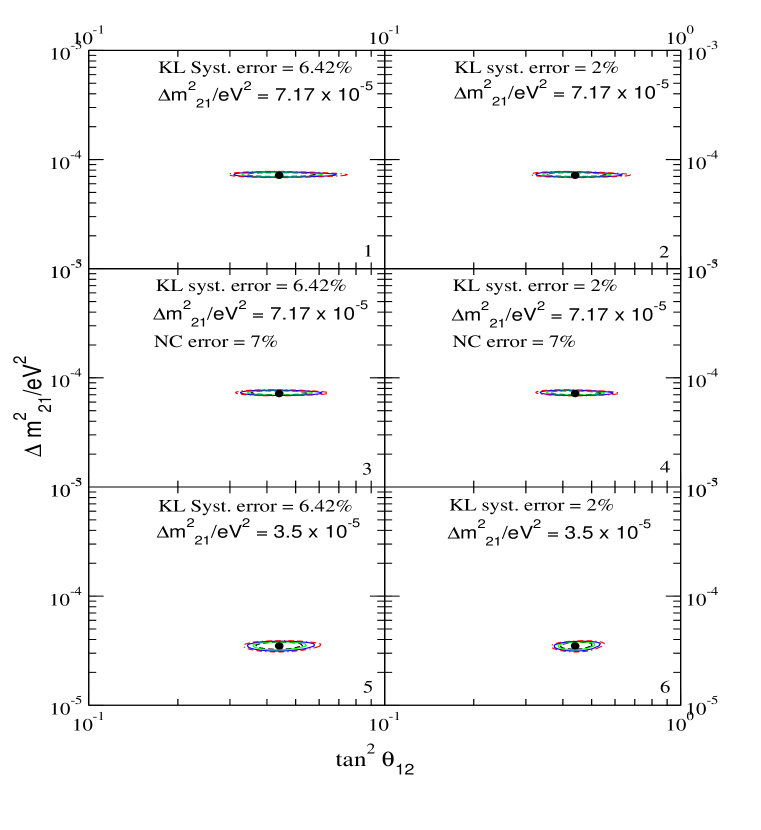
Figure 7: The 90%, 95%, 99% and 99.73% C.L. contours for the combined analysis using the solar and 3 kTy projected KamLAND spectrum. The upper panels are for the simulated KamLAND spectrum at low-LMA best-fit parameters and the current solar data, the middle panels are for the simulated KamLAND spectrum at low-LMA best-fit parameters and the solar data with future SNO NC data (7% error), while the lower panels are for KamLAND data simulated at $\Delta m_{21}^{2}=3.5\times 10^{-5}$ eV² and $\tan^{2}\theta_{12}=0.44$ and the current global solar data. The left-hand panels use the current KamLAND systematic uncertainty of 6.42% while the right-hand panels correspond to a fictitious systematic uncertainty of just 2%.

From the Figure 1 presented in Section 2 and the discussion on KamLAND sensitivity to $\theta_{12}$ in the previous section we conclude that a reactor experiment can measure $\theta_{12}$ accurately enough only if it is sensitive to the SPMIN. To further elaborate our point in figure 7 we present the allowed areas at 7.2$\times 10^{-5}$ eV² (SPMAX) and for a fictitious spectrum data in KamLAND simulated at $\mbox{$\Delta m_{21}^{2}$~{}}=3.5\times 10^{-5}$ eV² – which corresponds to an effective SPMIN in KamLAND . We show limits for the current KamLAND systematic uncertainty of 6.42% and a systematic uncertainty of just 2% . We take 3 statistics for KamLAND in all the cases. The % spread in uncertainty for the SPMAX case with 6.42% systematic uncertainty is 37% while for the SPMIN case with the same systematics the spread is 25%. The effect of reducing the systematics to 2% results in the spread coming down to 32% and 19% respectively. We have also explored the effect of reducing the SNO NC error to 7% for the SPMAX case. The resulting contours are presented in the middle panels of figure 7. The $\tan^{2}\mbox{$\theta_{12}$~{}}$ spread for this case with 2% systematic error in KamLAND is 27%. This emboldens us to believe that the most suitable experiment for $\theta_{12}$ measurement is an experiment sensitive to the SPMIN as expected in Section 2.

Thus unprecedented sensitivity to $\theta_{12}$ can be achieved in a terrestrial experiment if the distance traveled by the neutrino beam is tuned so that the detector observes a complete vacuum oscillation. The oscillation wavelength of the neutrinos can be calculated with reasonable accuracy with information on $\Delta m_{21}^{2}$ from KamLAND . For a reactor experiment which has a large flux around $3-4$ MeV, the detector needs to be placed at about 70 km from a powerful nuclear reactor in order to be sensitive to the oscillation SPMIN. Also important for accurate $\theta_{12}$ determination is to reduce the systematics. The major part of the 6.42% error in KamLAND comes from sources which affect the overall normalization of the observed anti-neutrino spectrum. These can be reduced if the experiment uses the near-far detector technique in which there are two identical detectors, one close to the reactor and another further away [27, 28]. Comparison of the number of detected events in the two detectors can be then used to reduce the systematics.

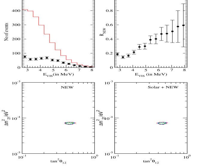
Figure 8: The simulated 3 kTy spectrum data at the low-LMA best-fit point and the allowed areas in the $\mbox{$\Delta m_{21}^{2}$~{}}-\tan^{2}\mbox{$\theta_{12}$~{}}$ parameter space for a 24.6 GWatt reactor experiment with a baseline of 70 km. The top-left panel gives the simulated spectrum data and the expected events, shown by the histograms. The top-right panel shows $R_{NEW}$, the corresponding ratio of the “data” to expected events as a function of the visible energy. The bottom-left panel gives the allowed areas obtained using just the new reactor experiment. The bottom-right panel presents the allowed areas from the combined solar and new reactor experiment data.

We show in Figure 8 the constraints on the mass and mixing parameters obtained using a “new” reactor experiment whose baseline is tuned to an oscillation SPMIN. We use the antineutrino flux from a reactor a la Kashiwazaki nuclear reactor in Japan with a maximum power generation of about 24.6 GWatt. We assume a 80% efficiency for the reactor output and simulate the 3 kTy data at the low-LMA best-fit for a KamLAND like detector placed at 70 km from the reactor source and which has systematic errors of only 2%. The top-left panel of the Figure 8 shows the simulated spectrum data. The histogram shows the expected spectrum for no oscillations. $E_{vis}$ is the “visible” energy of the scattered electrons. The top-right panel gives the ratio of the simulated oscillations to the no oscillation numbers. The sharp minima around $3-4$ MeV is clearly visible. The bottom-left panel gives the C.L. allowed areas obtained from this new reactor experiment data alone. With 3 kTy statistics we find a marked improvement in the $\theta_{12}$ bound with the 99% range $0.39<\tan^{2}\mbox{$\theta_{12}$~{}}<0.52$ giving a spread of 14%.

5 Other future experiments

We briefly discuss the sensitivity of the some of other next generation solar neutrino experiments. The most important among them are the Borexino which is sensitive to the monochromatic ${}^{7}{Be}$ neutrinos coming from the Sun and the sub-MeV solar neutrino experiments – the so called LowNu experiments.

5.1 Borexino

Borexino is a 300 ton organic liquid scintillator detector, viewed by 2200 photomultiplier tubes [29]. The Borexino detector due to start operations soon, has achieved a background reduction at sub-MeV energies never attempted before in a real time experiment. Borexino is tuned to detect mainly the ${}^{7}{Be}$ solar neutrinos by the elastic $\nu-e$ scattering process. The detector will operate in the electron recoil energy window of $0.25-0.8$ MeV to observe the mono-energetic 0.862 MeV ${}^{7}{Be}$ line which scatter electrons with a Compton edge at 0.66 MeV, the edge being somewhat smeared by the energy resolution of the detector.

Solution	$R_{Be}^{BF}$	$R_{Be}^{max}$	$R_{Be}^{min}$	$A_{DN}$
low-LMA	0.65	0.71	0.61	0.04
high-LMA	0.66	0.71	0.63	0.01

Table 2: The best-fit and $3\sigma$ range of predicted values for Borexino for the low-LMA and high-LMA solutions. Also shown is the value of the day-night asymmetry expected.

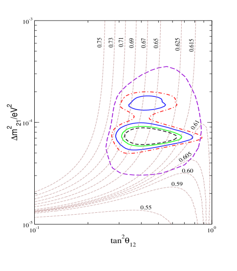
Figure 9: The isorate lines for the Borexino detector in the $\Delta m_{21}^{2}-\tan^{2}\theta_{12}$ plane. Also shown are the C.L. contours from the global analysis of the solar and the KamLAND data. Also shown by the purple dashed line is the only solar $3\sigma$ contour.

We present in Figure 9 the lines of constant Borexino rate in the $\Delta m_{21}^{2}-\tan^{2}\theta_{12}$ LMA zone. The Borexino rate $R_{Be}$ is defined as the ratio of the value predicted by oscillations to the no oscillation SSM value. The global allowed 90%, 95%, 99% and 99.73% C.L. contours are shown. Superimposed is the $3\sigma$ contour from the analysis of the only solar data. In Table 2 we show the predicted rate in Borexino for the low-LMA and high-LMA best-fit solutions and the corresponding $3\sigma$ ranges. From Figure 9 and Table 2 we note that Borexino in the LMA zone has almost no sensitivity to $\Delta m_{21}^{2}$. The reason being that for very low values of neutrino energies the solar matter effects are negligible while for $\Delta m_{21}^{2}$ in the LMA zone there are hardly any Earth matter effect. Hence the survival probability can be approximated by averaged oscillations (cf. Eq.(1)). Therefore Borexino is not expected to sharpen our knowledge of $\Delta m_{21}^{2}$ any further. Even the $\theta_{12}$ dependence is rather weak. This is due to the fact that the survival probability is of the averaged vacuum oscillation form which as discussed in Section 2 reduces the sensitivity of Borexino to $\theta_{12}$ .

The $3\sigma$ error in the predicted value of Borexino rate given in Table 2 from the current information on the parameter ranges is $\pm 0.06$. The corresponding $1\sigma$ range is $0.63<R_{Be}<0.68$ implying an uncertainty of about $\pm 0.02$. Since there is hardly any $\Delta m_{21}^{2}$ dependence involved the entire range can be attributed to the current uncertainty in $\theta_{12}$ . Borexino could improve on the $\theta_{12}$ uncertainty if it could measure $R_{Be}$ with a $1\sigma$ error less than about 0.02. The low-LMA predicts about 13,000 events in Borexino after one year of data taking. This gives a statistical error of about 0.9% only. However Borexino may still have large errors coming from its background selection.

In Table 2 we have also shown the day-night asymmetry expected in Borexino for the currently allowed parameter values. Borexino will see no difference between the event rates at day and during night. Until the recent results from KamLAND the major role which Borexino was expected to play was to give “smoking gun” signal for the low $\Delta m_{21}^{2}$ solution LOW by observing a large day-night asymmetry and for the vacuum oscillation solution by observing seasonal variation of the ${}^{7}{Be}$ flux. The large day-night asymmetry expected due to the small energy sensitivity of Borexino and the immaculate control over seasonal effects coming from the fact that ${}^{7}{Be}$ is a mono-energetic line – not to mention its ability to pin down the SMA solution which predicted almost no ${\nu_{e}}$ events in Borexino . However all three are comprehensively disfavored now. Unfortunately the only region of parameter space where Borexino lacks strength is the LMA, which is the correct solution to the solar neutrino problem.

5.2 Low-Nu experiments

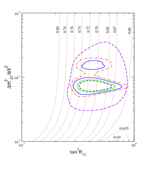
Figure 10: The isorate lines for a generic $pp$ - e scattering experiment in the $\Delta m_{21}^{2}-\tan^{2}\theta_{12}$ plane. Also shown are the C.L. contours from the global analysis of the solar and the KamLAND data. Also shown by the purple dashed line is the only solar $3\sigma$ contour.

There are a number of planned sub-MeV solar neutrino experiments which will look to observe the $pp$ flux using either charged current reactions (LENS, MOON, SIREN [30]) or electron scattering process(XMASS, CLEAN, HERON, MUNU, GENIUS [30]) for detecting the $pp$ neutrinos. While each of these electron scattering experiments use different detection techniques, the basic reaction involved is the scattering of the $pp$ neutrinos off the electrons in the detector. Hence we present in Figure 10 the lines of constant rate predicted in a generic LowNu electron scattering experiment. Again we note that the $iso-pp$ rates have very little $\Delta m_{21}^{2}$ dependence. The $3\sigma$ range predicted for $pp-e$ scattering is $0.66-0.76$. The corresponding $1\sigma$ predicted range is $0.68-0.73$. The advantage that these experiments have is that the $pp$ flux is predicted to within 1% accuracy. Thus the LowNu experiments may have a fair chance to pin down the value of the mixing angle $\theta_{12}$, if they can keep down their experimental errors.

6 Conclusions

With both solar and atmospheric neutrino oscillations confirmed the next turn in the research in neutrino physics is towards the precision determination of the oscillation parameters of the PMNS matrix. In this paper we explore in detail how accurately the current and future experiments will be able to predict $\theta_{\odot}$ ($\theta_{12}$) and show that with the current set of experiments the uncertainty level in the determination of $\theta_{12}$ may stay well above the desired 10% level (at 99% C.L.). The spectrum data from the KamLAND experiment with only 0.162 kTy exposure in conjunction with the global solar data reveals an unprecedented sensitivity in constraining $\Delta m^{2}_{21}$, reducing the 99% C.L. spread in $\Delta m^{2}_{21}$ to 30% as compared to 76% allowed by global solar data. A projected analysis with 3 kTy of simulated spectrum at the present best-fit reveals that the uncertainty in $\Delta m^{2}_{21}$ can be brought down to the $<$ 10% level. However even with 3 kTy of exposure the $\tan^{2}\theta_{12}$ can hover in a $\sim 33\%$ uncertainty range.

We make a comparative study of the $\theta_{12}$ sensitivity of the various solar neutrino experiments and KamLAND. The sensitivity of an experiment to $\theta_{12}$ depends on the form of the survival probability relevant for it. Thus the $\theta_{12}$ sensitivity of the solar neutrino experiments are linked with the neutrino energy threshold. In SK and SNO, the high energy neutrinos are observed and the solar neutrinos undergo adiabatic transformation ($P_{ee}\sim f_{B}\sin^{2}\theta_{12}$) resulting in an increased theta sensitivity as compared to the experiments which are sensitive to low energy neutrinos for which the survival probability is of the form $P_{ee}=1-0.5\sin^{2}2\theta_{12}$. SNO has a better control over $\theta_{12}$ than SK as it is sensitive to the total ${}^{8}B$ flux through its neutral current channel and hence limits the range of $f_{B}$, the ${}^{8}B$ flux normalization to 12%. We make a projected sensitivity test for the future SNO NC measurement and get the limits on $\theta_{12}$.

For the low energy neutrinos detected by the KamLAND detector the matter effects are absent. Therefore the relevant probability is the vacuum oscillation probability averaged over the various reactor distances. But inspite of this averaging effect the KamLAND spectrum data reveals an oscillation pattern which enables it to pin down the $\Delta m^{2}_{21}$. However for the KamLAND baseline this pattern corresponds to a peak in the survival probability where the $\theta_{12}$ sensitivity is very low. If instead of the peak one has a minimum in the survival probability, then the $\theta_{12}$ sensitivity can improve dramatically. We show this by simulating the 3 kTy spectrum for KamLAND at a $\Delta m_{21}^{2}=3.5\times 10^{-5}$ eV² for which one gets a survival probability minimum in KamLAND. For this value of $\Delta m_{21}^{2}$ the spread in $\theta_{\odot}$ decreases to 25%, even with the most conservative 6.42% systematic error. We also explore the effect of reducing the systematic error to a fictitious value of 2%. This further reduces the error in $\theta_{12}$ to 19%. For the current best-fit value of $\Delta m_{21}^{2}$ we propose a new KamLAND like reactor experiment with a baseline of $\sim$ 70 km. We show that this experiment can observe the minimum in the survival probability and therefore the $\theta_{12}$ sensitivity is increased by a large amount. For a systematic uncertainty of 2%, the total error in the allowed value of $\tan^{2}\theta_{12}$ can be reduced to about 14%.

Acknowledgment The authors would like to thank Raj Gandhi and D.P. Roy for discussions. S.C. acknowledges discussions with S.T. Petcov and useful correspondences with Aldo Ianni, Alessandro Strumia and Francesco Vissani. S.G. would like to acknowledge a question by Yuval Grossman in PASCOS’03 which started this work and D. Indumathi for some related comments. The authors express their sincere gratitude to Atsuto Suzuki, Fumihiko Suekane and Sandip Pakvasa for discussions on future systematic errors in KamLAND.

References

- [1] Q. R. Ahmad et al. [SNO Collaboration], Phys. Rev. Lett. 89, 011301 (2002) [arXiv:nucl-ex/0204008]; Q. R. Ahmad et al. [SNO Collaboration], Phys. Rev. Lett. 89, 011302 (2002) [arXiv:nucl-ex/0204009].
- [2] L. Wolfenstein, Phys. Rev. D 17, 2369 (1978) ; S. P. Mikheev and A. Y. Smirnov, Sov. J. Nucl. Phys. 42 (1985) 913 [Yad. Fiz. 42, 1441 (1985)] ; S. P. Mikheev and A. Y. Smirnov, Sov. J. Nucl. Phys. 42 (1985) 913 [Yad. Fiz. 42, 1441 (1985)] ; S. P. Mikheev and A. Y. Smirnov, Nuovo Cim. C 9, 17 (1986).
- [3] A. Bandyopadhyay, S. Choubey, S. Goswami and D. P. Roy, Phys. Lett. B 540, 14 (2002) [arXiv:hep-ph/0204286].
- [4] S. Choubey, A. Bandyopadhyay, S. Goswami and D. P. Roy, arXiv:hep-ph/0209222.
- [5] A. Bandyopadhyay, S. Choubey, S. Goswami and K. Kar, Phys. Lett. B 519, 83 (2001) [arXiv:hep-ph/0106264]; A. Bandyopadhyay, S. Choubey, S. Goswami and K. Kar, Phys. Rev. D 65, 073031 (2002) [arXiv:hep-ph/0110307].
- [6] K. Eguchi et al. [KamLAND Collaboration], Phys. Rev. Lett. 90, 021802 (2003) [arXiv:hep-ex/0212021].
- [7] A. Bandyopadhyay, S. Choubey, R. Gandhi, S. Goswami and D. P. Roy, arXiv:hep-ph/0212146.
- [8] V. Barger and D. Marfatia, arXiv:hep-ph/0212126; G. L. Fogli, E. Lisi, A. Marrone, D. Montanino, A. Palazzo and A. M. Rotunno, arXiv:hep-ph/0212127; M. Maltoni, T. Schwetz and J. W. Valle, arXiv:hep-ph/0212129; J. N. Bahcall, M. C. Gonzalez-Garcia and C. Pena-Garay, arXiv:hep-ph/0212147; P. C. de Holanda and A. Y. Smirnov, arXiv:hep-ph/0212270. H. Nunokawa, W. J. Teves and R. Zukanovich Funchal, arXiv:hep-ph/0212202; P. Aliani, V. Antonelli, M. Picariello and E. Torrente-Lujan, arXiv:hep-ph/0212212; A. B. Balantekin and H. Yuksel, arXiv:hep-ph/0301072; P. Creminelli, G. Signorelli and A. Strumia, [arXiv:hep-ph/0102234 (v4)].
- [9] Y. Fukuda et al. [Super-Kamiokande Collaboration], Phys. Rev. Lett. 81 (1998) 1562 [arXiv:hep-ex/9807003].
- [10] M. H. Ahn et al. [K2K Collaboration], arXiv:hep-ex/0212007.
- [11] T. Kajita (for Super-Kamiokande Collaboration) talk given at Neutrino Factory meeting, London, July 2002 (http://www.hep.ph.ic.ac.uk/NuFact02/).
- [12] B. Pontecorvo, Sov. Phys. JETP 6, 429 (1957) [Zh. Eksp. Teor. Fiz. 33, 549 (1957)]; B. Pontecorvo, Sov. Phys. JETP 7, 172 (1958) [Zh. Eksp. Teor. Fiz. 34, 247 (1957)]; Z. Maki, M. Nakagawa and S. Sakata, Prog. Theor. Phys. 28, 870 (1962).
- [13] M. Apollonio et al. [CHOOZ Collaboration], Phys. Lett. B 466, 415 (1999) [arXiv:hep-ex/9907037] ; M. Apollonio et al. [CHOOZ Collaboration], Phys. Lett. B 420, 397 (1998) [arXiv:hep-ex/9711002]; M. Apollonio et al., arXiv:hep-ex/0301017.
- [14] F. Boehm et al., Phys. Rev. D 64, 112001 (2001) [arXiv:hep-ex/0107009].
- [15] M. Apollonio et al., arXiv:hep-ph/0210192.
- [16] Y. Itow et al., arXiv:hep-ex/0106019.
- [17] D. Ayres et al., arXiv:hep-ex/0210005.
- [18] S. Geer, hep-ph/0008155.
- [19] J. N. Abdurashitov et al. [SAGE Collaboration], v ity,” arXiv:astro-ph/0204245 ; W. Hampel et al. [GALLEX Collaboration], Phys. Lett. B 447, 127 (1999) ; E. Bellotti, Talk at Gran Sasso National Laboratories, Italy, May 17, 2002 ; T. Kirsten, talk at Neutrino 2002, XXth International Conference on Neutrino Physics and Astrophysics, Munich, Germany, May 25-30, 2002. (http://neutrino2002.ph.tum.de/)
- [20] S. Fukuda et al. [Super-Kamiokande Collaboration], Phys. Lett. B 539, 179 (2002) [arXiv:hep-ex/0205075].
- [21] B. T. Cleveland et al., Astrophys. J. 496, 505 (1998).
- [22] J. N. Bahcall, M. H. Pinsonneault and S. Basu, Astrophys. J. 555, 990 (2001) [arXiv:astro-ph/0010346].
- [23] A. Bandyopadhyay, S. Choubey and S. Goswami, Phys. Lett. B 555, 33 (2003) [arXiv:hep-ph/0204173].
- [24] S. Choubey, S. Goswami and D. P. Roy, Phys. Rev. D 65, 073001 (2002) [arXiv:hep-ph/0109017]; S. Choubey, S. Goswami, N. Gupta and D. P. Roy, Phys. Rev. D 64, 053002 (2001) [arXiv:hep-ph/0103318].
- [25] M. Maris and S. T. Petcov, Phys. Lett. B 534, 17 (2002) [arXiv:hep-ph/0201087].
- [26] A. Bandyopadhyay, S. Choubey, R. Gandhi, S. Goswami and D. P. Roy, arXiv:hep-ph/0211266; V. D. Barger, D. Marfatia and B. P. Wood, Phys. Lett. B 498, 53 (2001) [arXiv:hep-ph/0011251]; H. Murayama and A. Pierce, Phys. Rev. D 65, 013012 (2002) [arXiv:hep-ph/0012075].
- [27] Y. Kozlov, L. Mikaelyan and V. Sinev, arXiv:hep-ph/0109277;
- [28] H. Minakata, H. Sugiyama, O. Yasuda, K. Inoue and F. Suekane, arXiv:hep-ph/0211111.
- [29] G. Alimonti et al. [Borexino Collaboration], Astropart. Phys. 16, 205 (2002) [arXiv:hep-ex/0012030].
- [30] S. Schönert, talk at Neutrino 2002, Munich, Germany, (http://neutrino2002.ph.tum.de).