Chiral Quark Model

Abstract

In this talk I review studies of hadron properties in bosonized chiral quark models for the quark flavor dynamics. Mesons are constructed from Bethe–Salpeter equations and baryons emerge as chiral solitons. Such models require regularization and I show that the two–fold Pauli–Villars regularization scheme not only fully regularizes the effective action but also leads the scaling laws for structure functions. For the nucleon structure functions the present approach serves to determine the regularization prescription for structure functions whose leading moments are not given by matrix elements of local operators. Some numerical results are presented for the spin structure functions.

1. Introduction

In this talk I review investigations of hadron properties in the Nambu–Jona–Lasino (NJL) model [?]. This is a particularly simple model for the quark flavor interactions with the important feature that the quarks can be integrated out in favor of meson fields [?]. The resulting effective action for these mesons possesses soliton solutions [?]. According to the large–$N_{C}$ picture [?] of Quantum–Chromo–Dynamics (QCD) these solutions are interpreted as baryons.

The construction of hadron wave–functions is not possible in QCD. This represents a main obstacle for the computation of hadron properties from first principles. As the NJL model adopts the symmetry properties of QCD, the current operators in the model correspond to those of QCD. As a consequence, matrix elements of the current operators as computed in the model are sensible and their comparison with experimental data is meaningful. In particular, it is interesting to analyze the hadronic tensor that parameterizes the deep–inelastic–scattering (DIS) and confront the model predictions with empirical data. This picture has led to interesting studies of hadron structure functions in bosonized chiral quark models. Here I will present the results of refs. [?,?,?]. These studies build up a consistent approach by computing the hadronic tensor (or equivalently the forward virtual Compton amplitude) from the gauged meson action. For the nucleon structure functions similar studies have been reported in refs. [?,?,?]. There no attempt to compute the structure functions from the gauged action was made but rather it was assumed that the model predictions for the constituent quark distributions can be identified with QCD quark distributions. I refer to those articles for a more expatiated presentation of numerical results. In addition, I refer to the review articles  [?] for comprehensive discussions of model predictions for static baryon properties such as magnetic moments, axial charges or the hyperon spectrum.

This talk is organized as follows. In Section 2 I introduce the NJL model as an effective meson theory and utilize pion properties to determine the model parameters. Section 3 describes the subtleties for extracting the structure functions that arise in this model from regularization. The pion structure function is considered as an example. In Section 4 I review the construction of baryon states in the soliton picture. The following Section sketches the computation of nucleon matrix elements of the hadronic tensor and the extraction of the structure functions in the Bjorken limit. Finally in Section 6 I present some numerical results for the spin structure functions $g_{1}$ and $g_{2}$ and compare them to experimental data by means of the transformation to the infinite momentum frame and subsequent DGLAP evolution. Section 7 serves as a short summary.

2. The NJL Model for Chiral Dynamics

The NJL model is a quark model with a chirally invariant quartic quark interaction. Bosonization is achieved semiclassically by introducing effective meson fields for the quark bilinears in that interaction. Then the quark fields are integrated out by functional methods. This yields an effective action for meson degrees of freedom,

$${\mathcal{A}}[S,P]=-iN_{C}{\rm Tr}_{\textstyle\Lambda}{\rm log}\,\left[i\partial\hskip-5.0pt/-\left(S+i\gamma_{5}P\right)\right]-\frac{1}{4G}\int d^{4}x\,{\rm tr}\,{\mathcal{V}}(S,P)\,.$$ (1)

Here ${\mathcal{V}}$ is a local potential for the effective scalar and pseudoscalar fields $S$ and $P$, respectively, that are matrices in flavor space. In the NJL model the potential reads ${\mathcal{V}}=S^{2}+P^{2}+2{\hat{m}}_{0}S$ with $\hat{m}_{0}$ being the current quark mass matrix. Since the interaction is mediated by flavor degrees of freedom, the number of colors, $N_{C}$, is merely a multiplicative quantity. The functional trace (${\rm Tr}$) originates from integrating out the quarks and induces a non–local interaction for $S$ and $P$. For simplicity I will only consider the isospin limit for up (u) and down (d) quarks: $m_{0,u}=m_{0,d}=m_{0}$.

A major concern in regularizing the functional (1), as indicated by the cut–off $\Lambda$, is to maintain the chiral anomaly. This is achieved by splitting this functional into $\gamma_{5}$–even and odd pieces and only regulate the former,

$${\rm Tr}_{\Lambda}{\rm log}\,\left[i\partial\hskip-5.0pt/-\left(S+i\gamma_{5}P\right)\right]=-i\frac{N_{C}}{2}\sum_{n=0}^{2}c_{n}{\rm Tr}\,{\rm log}\left[-{\bf D}{\bf D}_{5}+\Lambda_{n}^{2}-i\epsilon\right]\hskip 11.38092pt$$ (3)

$$\hskip 128.0374pt-i\frac{N_{C}}{2}{\rm Tr}\,{\rm log}\left[-{\bf D}\left({\bf D}_{5}\right)^{-1}-i\epsilon\right]\,,$$

$${\rm with}\, \qquad i{\bf D}=i\partial\hskip-5.0pt/-\left(S+i\gamma_{5}P\right)\quad{\rm and}\quad i{\bf D}_{5}=-i\partial\hskip-5.0pt/-\left(S-i\gamma_{5}P\right)\,.$$ (4)

The double Pauli–Villars regularization renders the functional (1) finite with $c_{0}=1,\,\,\Lambda_{0}=0,\,\sum_{n=0}^{2}c_{n}=0\,.$ The $\gamma_{5}$–odd piece is conditionally finite and not regularizing it, reproduces the chiral anomaly properly. For sufficiently large $G$ one obtains the VEV, $\langle S\rangle\equiv m\mbox{{\sf 1}\mbox{}\rule{0.39993pt}{6.6736pt}\mbox{\hskip 1.00006pt}}$ that parameterizes the dynamical chiral symmetry breaking from the gap–equation,

$$\frac{1}{2G}\left(m-m_{0}\right)=4iN_{C}m\sum_{n=0}^{2}c_{n}\int\frac{d^{4}k}{(2\pi)^{4}}\left[k^{2}-m^{2}-\Lambda_{n}^{2}+i\epsilon\right]^{-1}\,.$$ (5)

Substituting $S=\langle S\rangle=m\mbox{{\sf 1}\mbox{}\rule{0.39993pt}{6.6736pt}\mbox{\hskip 1.00006pt}}$ in eq. (1) shows that $m$ plays the role of a mass and is therefore called the constituent quark mass.

In the next step I utilize pion properties to fix the model parameters and introduce the isovector pion field ${\vec{\pi}}$ via

$$S+iP\gamma_{5}=m\,\left(U\right)^{\gamma_{5}}=m\,{\rm exp}\left(i\frac{g}{m}\gamma_{5}\,{\vec{\pi}}\cdot{\vec{\tau}}\right)\,.$$ (6)

Sandwiching the axial current between the vacuum and a single pion state yields the pion decay constant $f_{\pi}=93{\rm MeV}$ in terms of the polarization function $\Pi(q^{2},x)$,

$$f_{\pi} = 4N_{C}mg\int_{0}^{1}\,dx\,\Pi(m_{\pi}^{2},x)$$ (7)

$$\Pi(q^{2},x) = \sum_{n=0}^{2}c_{n}\,\frac{d^{4}k}{(2\pi)^{4}i}\,\left[k^{2}+x(1-x)m_{\pi}^{2}-m^{2}-\Lambda_{n}^{2}+i\epsilon\right]^{-2}\,,$$ (8)

where $m_{\pi}=138{\rm MeV}$ is the pion mass. The Yukawa coupling constant, $g$, is determined by the requirement that the pion propagator has unit residuum,

$$\frac{1}{g^{2}}=4N_{C}\frac{d}{dm_{\pi}^{2}}\int_{0}^{1}\,dx\,\left[m^{2}_{\pi}\Pi(m_{\pi}^{2},x)\right]\,.$$ (9)

In the chiral limit ($m_{\pi}=0$) this simplifies to $f_{\pi}=m/g$. Finally the current quark mass is fixed from the condition that the pole of the pion propagator is exactly at the pion mass,

$$m_{0}=4\,N_{C}\,m\,G\,m_{\pi}^{2}\,\int_{0}^{1}\,dx\,\Pi(m_{\pi}^{2},x)\,.$$ (10)

It is also worthwhile to mention that expanding eqs. (3) and (6) to linear and quadratic order in $\vec{\pi}$ and $v_{\mu}$, respectively, yields the correct width for the anomalous decay $\pi^{0}\to\gamma\gamma$. This is the direct consequence of not regularizing the $\gamma_{5}$–odd piece.

Before discussing nucleons as solitons of the bosonized action (1) and the respective structure functions it will be illuminating to first consider DIS off pions.

3. The Compton Tensor and Pion Structure Function

DIS off hadrons is parameterized by the hadronic tensor $W^{\mu\nu}(p,q)$ where $q$ is the momentum transmitted from the photon to the hadron with momentum $p$.

The tensor $W^{\mu\nu}(p,q)$ is obtained from the hadron matrix element of the current commutator by Fourier transformation and is parameterized in terms of form factors that multiply the allowed Lorentz structures. These form factors are obtained by pertinent projection of the hadronic tensor. Finally the structure functions are the leading twist contributions of the form factors. These contributions are obtained from computing $W^{\mu\nu}(p,q)$ in the Bjorken limit: $Q^{2}=-q^{2}\to\infty$ with $x=Q^{2}/p\cdot q$ fixed. That is, subleading contributions in $1/Q^{2}$ are omitted.

An essential feature of bosonized quark models is that the derivative term in (1) is formally identical to that of a non–interacting (or asymptotically free) quark model. Hence the current operator is given as $J^{\mu}={\bar{q}}{\mathcal{Q}}\gamma^{\mu}q$, with ${\mathcal{Q}}$ a flavor matrix. Expectation values of currents are computed by introducing pertinent sources $v_{\mu}$ in eq. (3)

$$i{\bf D}\,\longrightarrow\,i{\bf D}+{\mathcal{Q}}v\hskip-5.0pt/\qquad{\rm and}\qquad i{\bf D}_{5}\,\longrightarrow\,i{\bf D}_{5}-{\mathcal{Q}}v\hskip-5.0pt/$$ (11)

and differentiating the gauged action (1) with respect to $v_{\mu}$. In bosonized quark models it is convenient to start from the absorptive part of the forward virtual Compton amplitude

$$T^{\mu\nu}(p,q)=\int d^{4}\xi\,{\rm e}^{iq\cdot\xi}\,\langle p,s|T\left(J^{\mu}(\xi)J^{\nu}(0)\right)|p,s\rangle\,\,\,,\,\,\,\,W^{\mu\nu}(p,q)=\frac{1}{2\pi}{\mathsf{Im}}\,[T^{\mu\nu}(p,q)]$$ (12)

because the time–ordered product is straightforwardly obtained from

$$T\left(J^{\mu}(\xi)J^{\nu}(0)\right)=\frac{\delta^{2}}{\delta v_{\mu}(\xi)\,\delta v_{\nu}(0)}\,{\rm Tr}_{\Lambda}{\rm log}\,\left[i\partial\hskip-5.0pt/-\left(S+i\gamma_{5}P\right)+{\mathcal{Q}}\,v\hskip-5.0pt/\right]\Big{|}_{v_{\mu}=0}\,,$$ (13)

as defined from eq. (3) with the substitution (11).

Pion–DIS is characterized by a single structure function, $F(x)$. For its computation the pion matrix element in the Compton amplitude (12) must be specified. For virtual pion–photon scattering it is obtained by expanding eqs. (3) and (6) to second order in both, ${\vec{\pi}}$ and $v_{\mu}$. Due to the separation into ${\bf D}$ and ${\bf D}_{5}$ this calculation differs considerably from the simple evaluation of the ‘handbag’ diagram. For example, isospin violating and dimension–five operators appear for the action (3). Fortunately all isospin violating pieces cancel yielding

$$F(x)=\frac{5}{9}(4N_{C}g^{2})\frac{d}{dm_{\pi}^{2}}\left[m_{\pi}^{2}\Pi(m_{\pi}^{2},x)\right]\,,\quad 0\leq x\leq 1\,.$$ (14)

The same result is obtained by formal treatment of the divergent handbag diagram and ad hoc regularization [?]. The cancellation of the isospin violating pieces is a feature of the Bjorken limit: insertions of the pion field on the propagator carrying the infinitely large photon momentum can be safely ignored. Furthermore this propagator can be taken to be the one for non–interacting massless fermions. This implies that also the Pauli–Villars cut–offs can be omitted for this propagator. That, in turn, leads to the desired scaling behavior of the structure function in this model and is a particular feature of the Pauli–Villars regularization. A priori it is not obvious for an arbitrary regularization scheme that terms of the form $Q^{2}/\Lambda_{n}^{2}$ drop out in the Bjorken limit.

From eqs. (9) and (14) it is obvious that $F(x)=5/9$ for $0\leq x\leq 1$ in the chiral limit ($m_{\pi}=0$). It must be noted that this refers to the structure function at the (low) energy scale of the model. To compare with empirical data, that are at a higher energy scale, the DGLAG program of perturbative QCD has to be applied to $F(x)$ to include the ${\rm ln}Q^{2}$ corrections. Such studies  [?] show good agreement with the experimental data for $F(x)$.

4. The Nucleon as a Chiral Soliton

Solitons are a non–perturbative stationary configurations of the meson fields. To determine that configuration for the meson theory (1) I consider the hedgehog ansatz

$$U_{\rm H}(\vec{r})={\rm exp}\left(i\vec{\tau}\cdot\hat{r}F(r)\right)\quad{\rm and}\quad\left(U_{\rm H}(\vec{r\,})\right)^{\gamma_{5}}={\rm exp}\left(i\gamma_{5}\vec{\tau}\cdot\hat{r}F(r)\right)$$

for the pion field (6). The corresponding single particle Dirac Hamiltonian reads

$$h=\vec{\alpha}\cdot\vec{p}+\beta\,m\,\left[{\rm cos}F+i\gamma_{5}\vec{\tau}\cdot\hat{r}\,{\rm sin}F\right]\,.$$ (15)

Evaluating the action functional (3) in the eigenbasis of $h$ gives the energy functional in terms of the eigenvalues, $\epsilon_{\alpha}$,  [?]

$$E[F] = \frac{N_{C}}{2}\left(1-{\rm sign}(\epsilon_{\rm V})\right)\epsilon_{\rm V}-\frac{N_{C}}{2}\sum_{\alpha}\sum_{n=0}^{2}c_{n}\left\{\sqrt{\epsilon_{\alpha}^{2}+\Lambda_{n}^{2}}-\sqrt{\epsilon_{\alpha}^{(0)2}+\Lambda_{n}^{2}}\right\}$$ (17)

$$\hskip 56.9055pt+m_{\pi}^{2}f_{\pi}^{2}\int d^{3}r\,(1-{\rm cos}F)\,$$

for a baryon number one configuration. Here ${\rm V}$ denotes the unique quark level that is strongly bound by the soliton. Its explicit occupation takes care of the total fermion number and thus this level is referred to as the valence quark. It should not be confused with the valence quarks in the parton model. Furthermore $\epsilon_{\alpha}^{(0)}$ are the eigenvalues of $h^{(0)}=\vec{\alpha}\cdot\vec{p}+\beta\,m\,$. The soliton profile $F(r)$ is then obtained from extremizing $E$ self–consistently  [?].

States possessing good spin and isospin quantum numbers are generated by taking the zero–modes to be time dependent [?]

$$U(\vec{r\,},t)=A(t)U_{\rm H}(\vec{r\,})A^{{\dagger}}(t)\ ,$$ (18)

which introduces the collective coordinates $A(t)\in SU(2)$. The action functional is expanded [?] up to quadratic order in the angular velocities

$$i\vec{\tau}\cdot\vec{\Omega}=2A^{{\dagger}}(t)\dot{A}(t)\,.$$ (19)

The coefficient of the quadratic term defines the moment of inertia, $\alpha^{2}[F]$. Nucleon states $|N\rangle$ are obtained by canonical quantization of the collective coordinates, $A(t)$. This is analogous to quantizing a rigid rotator and allows to compute matrix elements of operators in the space of the collective coordinates [?]:

$$\langle N|\textstyle{\frac{1}{2}}{\rm tr}\left(\tau_{a}A^{\dagger}\tau_{b}A\right)|N\rangle=-\textstyle{\frac{4}{3}}\langle N|I_{a}J_{b}|N\rangle\quad{\rm and}\quad\vec{\Omega}=-\vec{J\,}/\alpha^{2}[F]\,,$$ (20)

where $I_{a}$ and $J_{b}$ denote isospin and spin, respectively.

For later use I note that the valence quark wave–function receives a first order cranking correction

$$\Psi_{\rm V}(\vec{r\,},t)={\rm e}^{-i\epsilon_{\rm V}t}A(t)\left\{\phi_{\rm V}(\vec{r\,})+\frac{1}{2}\sum_{\mu\neq{\rm V}}\phi_{\mu}(\vec{r\,})\frac{\langle\mu|\vec{\tau}\cdot\vec{\Omega}|{\rm V}\rangle}{\epsilon_{\rm V}-\epsilon_{\mu}}\right\}\,,$$ (21)

where $\phi_{\mu}(\vec{r\,})$ are the eigenfunctions of $h$ in eq. (15). The moment of inertia, $\alpha^{2}[F]$ is order $N_{C}$, thus, upon quantization (20), this rotational correction is subleading in $1/N_{C}$.

5. Nucleon Structure Functions

DIS off nucleons is described by four structure functions: $F_{1}(x)$ and $F_{2}(x)$ are insensitive to the nucleon spin while the polarized structure functions, $g_{1}(x)$ and $g_{2}(x)$, are associated with the components of the hadronic tensor that contain the nucleon spin.

As argued in section 3, the quark propagator with the infinite photon momentum should be taken to be the one for free and massless fermions. Thus, it is sufficient to differentiate (Here ${\bf D}$ and ${\bf D}_{5}$ are those of eq (4), i.e. with $v_{\mu}=0$.)

$$\frac{N_{C}}{4i}\sum_{n=0}^{2}c_{n}{\rm Tr}\,\left\{\left(-{\bf D}{\bf D}_{5}+\Lambda_{n}^{2}\right)^{-1}\left[{\mathcal{Q}}^{2}v\hskip-5.0pt/\left(\partial\hskip-5.0pt/\right)^{-1}v\hskip-5.0pt/{\bf D}_{5}-{\bf D}(v\hskip-5.0pt/\left(\partial\hskip-5.0pt/\right)^{-1}v\hskip-5.0pt/)_{5}{\mathcal{Q}}^{2}\right]\right\}$$ (22)

$$+\frac{N_{C}}{4i}{\rm Tr}\,\left\{\left(-{\bf D}{\bf D}_{5}\right)^{-1}\left[{\mathcal{Q}}^{2}v\hskip-5.0pt/\left(\partial\hskip-5.0pt/\right)^{-1}v\hskip-5.0pt/{\bf D}_{5}+{\bf D}(v\hskip-5.0pt/\left(\partial\hskip-5.0pt/\right)^{-1}v\hskip-5.0pt/)_{5}{\mathcal{Q}}^{2}\right]\right\}\,,\,\,$$ (23)

with respect to the photon field $v_{\mu}$. I have introduced the $(\ldots)_{5}$ description

$$\gamma_{\mu}\gamma_{\rho}\gamma_{\nu}=S_{\mu\rho\nu\sigma}\gamma^{\sigma}-i\epsilon_{\mu\rho\nu\sigma}\gamma^{\sigma}\gamma^{5}\,,\quad(\gamma_{\mu}\gamma_{\rho}\gamma_{\nu})_{5}=S_{\mu\rho\nu\sigma}\gamma^{\sigma}+i\epsilon_{\mu\rho\nu\sigma}\gamma^{\sigma}\gamma^{5}$$

to account for the unconventional appearance of axial sources in ${\bf D}_{5}$, cf. ref. [?]. Substituting eq. (18) for the meson fields that are contained in ${\bf D}$ and ${\bf D}_{5}$, computing the functional trace up to subleading order in $1/N_{C}$ using a basis of quark states obtained from the Dirac Hamiltonian (15), yields analytical results for the structure functions. I refer to ref. [?] for detailed formulas for other structure functions and the verification of the sum rules that relate integrals over the structure functions to static nucleon properties. As an example I restrain myself to list the contribution to $g_{1}(x)$ which is leading order in $1/N_{C}$:

$$g_{1}(x) = \frac{M_{N}N_{C}}{36i}\Big{\langle}N\Big{|}I_{3}\Big{|}N\Big{\rangle}\int\frac{d\omega}{2\pi}\sum_{\alpha}\int d^{3}\xi\int\frac{d\lambda}{2\pi}\,{\rm e}^{iM_{N}x\lambda}\hskip 85.35826pt$$ (26)

$$\times\left(\sum_{n=0}^{2}\frac{c_{n}\left(\omega+\epsilon_{\alpha}\right)}{\omega^{2}-\epsilon_{\alpha}^{2}-\Lambda_{n}^{2}+i\epsilon}\right)_{\rm P}\Big{[}\phi^{\dagger}_{\alpha}(\vec{\xi\,})\tau_{3}\left(1-\alpha_{3}\right)\gamma_{5}\phi_{\alpha}(\vec{\xi\,}\hskip-1.70717pt+\hskip-1.70717pt\lambda\hat{e}_{3}){\rm e}^{-i\omega\lambda}$$

$$\hskip 113.81102pt+\phi^{\dagger}_{\alpha}(\vec{\xi})\tau_{3}\left(1-\alpha_{3}\right)\gamma_{5}\phi_{\alpha}(\vec{\xi}\hskip-1.70717pt-\hskip-1.70717pt\lambda\hat{e}_{3}){\rm e}^{i\omega\lambda}\Big{]}\,,$$

where the subscript ($P$) indicates the pole term.

Before discussing numerical results I would like to mention the unexpected result that the structure function entering the Gottfried sum rule is related to the $\gamma_{5}$–odd piece of the action and hence does not undergo regularization. This is surprising because in the parton model this structure function differs from the one associated with the Adler sum rule only by the sign of the anti–quark distribution. The latter structure function, however, gets regularized in the present model, in agreement with the quantization rule for the collective coordinates that correspond to the isospin operator that involves the regularized moment of inertia, $\alpha^{2}$.

6. Numerical Results for Nucleon Structure Functions

Unfortunately numerical results for the full structure functions in the double Pauli–Villars regularization scheme, i.e. including the properly regularized vacuum piece are not yet available. However, in the Pauli–Villars regularization the axial charges are saturated to 95% or even more by their valence quark (21) contributions once the self–consistent soliton is substituted. This provides sufficient justification to consider the valence quark contribution to the polarized structure functions as a reliable approximation since e.g. the zeroth moment of the leading structure function $g_{1}$ is nothing but the axial current matrix element. This valence quark level is that of the chiral soliton model and, as already mentioned, its contributions to the structure functions should not be confused with valence quark distributions in parton models. In general, it should be stressed that the present model calculation yields structure functions, i.e. quantities that parameterize the hadronic tensor, but not (anti)–quark distributions. The latter would require the identification of model degrees of freedom with those in QCD. However, here only the symmetries (namely the chiral symmetry) and thus the current operators in the hadronic tensor are identified.

As in the case for the pion, the model calculation yields the nucleon structure function at a low energy scale. In addition the soliton is a localized object. Thus the computed structure functions are frame–dependent and one frame has to be picked. The appropriate choice is the infinite momentum frame (IMF) not only because it makes contact with the parton model but also because it is that frame in which the support of the structure functions is limited to the physical regime $0\leq x\leq 1$. Choosing the IMF amounts to the transformation [?,?]

$$f_{\rm IMF}(x)=\frac{1}{1-x}\,f_{\rm RF}(-{\rm ln}(1-x))\,,$$ (27)

where $f_{\rm RF}(x)$ denotes the structure function as computed in the nucleon rest frame. So the program is two–stage, first the transformation of the model structure function to the IMF according to eq (27) and subsequently the DGLAP evolution program [?] to incorporate the resumed ${\rm ln}Q^{2}$ corrections. In the current context it is appropriate to restrain oneself to the leading order (in $\alpha_{s}$) in the evolution program because higher orders require the identification of quark and antiquark distributions in the parton models sense. In the present model calculation this is not possible without further assumptions. The low energy scale, $Q^{2}_{0}=0.4{\rm GeV}^{2}$, at which the model is assumed to approximate QCD has been estimated in ref.  [?] from a best fit to the experimental data of the unpolarized structure function, $F_{2}(x)$. The same boundary value is taken to evolve the model prediction for polarized structure function, $g_{1}(x)$, in the IMF to the scale $Q^{2}$ of several ${\rm GeV}^{2}$ at which the experimental data are available. For the structure function $g_{2}(x)$ the situation is a bit more complicated. First the twist–2 piece must be separated according to [?]

$$g_{2}^{WW}(x)=-g_{1}(x)+\int_{x}^{1}\frac{dy}{y}\,g_{1}(y)$$ (28)

and evolved analogously to $g_{1}(x)$ (which also is twist–2). The remainder, $g_{2}(x)-g_{2}^{WW}(x)$, is twist–3 and is evolved according to the large–$N_{C}$ scheme of ref. [?]. Finally, the two pieces are again put together at the end–point of the evolution, $Q^{2}$. In figure 1 I compare the model predictions for the linearly independent polarized structure functions of the proton to experimental data [?].

Figure  1.: Model predictions for the polarized proton structure functions $xg_{1}$ (left panel) and $xg_{2}$ (right panel). The curves labeled ‘RF’ denote the results as obtained from the valence quark contribution to (23). These undergo a projection to the infinite momentum frame ‘IMF’ (27) and a leading order ‘LO’ DGLAP evolution [?]. Data are from SLAC–E143 [?].

In figure 2 I compare the model predictions for both the proton and the neutron (in form of the deuteron) not only to the recently accumulated data but also to other model predictions.

Figure  2.: Model predictions for the polarized proton structure functions $xg_{2}$ for proton and neutron (deuteron) and comparison with data from E143 [?] (open diamond) and E155 [?] (open square) and their combination (solid circle). The full line is the twist–2 truncation (28) of data for $g_{1}(x)$. Dashed–dotted [?] and dotted [?] lines are bag model calculations, the short dashed lines represent the present chiral soliton model [?] and long dashed line that of ref. [?]. (This is a slightly modified figure from ref. [?].)

Surprisingly the twist–2 truncation, i.e. eq. (28) with the data for $g_{1}(x)$ at the right hand side, gives the most accurate description of the data. However, also the chiral soliton model predictions reproduce the data well. Bag model predictions have a less pronounced structure.

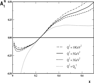
Figure  3.: Model prediction for $A_{1}^{N}$ at different $Q^{2}$. The right panel shows the various experimental data  [?]. The JLab–data (E99–117) are still preliminary.

Recently, precise data  [?] have become available for the neutron asymmetry

$$A_{1}=\frac{g_{1}(x,Q^{2})-\frac{4M^{2}x^{2}}{Q^{2}}g_{2}(x,Q^{2})}{F_{1}(x,Q^{2})}\,.$$ (29)

It is therefore challenging to study this quantity in the present model. As subleading twist contributions are omitted, this amounts to computing the ratio $g_{1}(x,Q^{2})/F_{1}(x,Q^{2})$, for the neutron. The resulting ratio is shown in Fig. 3 together with data. It is interesting to note that while the ratio at the model scale, $Q_{0}$, becomes large and negative at small $x$, the DGLAP evolution causes it to bend around so that it actually tends to zero as $x\to 0$. This behavior is also observed from the data, as is the change in sign at moderate $x$. The position ($x\approx 0.25$) at which this change occurs seems somewhat lower than the preliminary JLab–data  [?] suggest and insensitive to the end point of evolution. Once evolution has set in at a moderate point $Q^{2}$, the evolution to even higher $Q^{2}$ has insignificant effect.

7. Conclusions

I have discussed a chiral quark model for hadron phenomenology. In particular, I considered the bosonized NJL model as a simplified model for the quark flavor dynamics. Although the bosonized version is a meson theory, the quark degrees of freedom can indeed be traced. This is very helpful for considering structure functions. Additional correlations are introduced due to the unavoidable regularization which is imposed in a way to respect the chiral anomaly. Hence a consistent extraction of the nucleon structure functions from the Compton amplitude in the Bjorken limit leads to expressions that are quite different from those obtained by an ad hoc regularization of quark distributions in the same model. I also showed that within a reliable approximation the numerical results for the spin dependent structure functions agree reasonably well with the empirical data.

REFERENCES

- [1] Y. Nambu and G. Jona–Lasinio, Phys. Rev. 122 (1961) 345; 124 (1961) 246.
- [2] D. Ebert and H. Reinhardt, Nucl. Phys. B271 (1986) 188.
- [3] R. Alkofer, H. Reinhardt and H. Weigel, Phys. Rept. 265 (1996) 139; C. V. Christov et al., Prog. Part. Nucl. Phys. 37 (1996) 91.
- [4] G. t‘ Hooft, Nucl. Phys. B72 (1974) 461; B75 (1975) 461; E. Witten, Nucl. Phys. B160 (1979) 57.
- [5] H. Weigel, L. Gamberg and H. Reinhardt, Mod. Phys. Lett. A11 (1996) 3021; Phys. Lett. B399 (1997) 287; L. Gamberg, H. Reinhardt and H. Weigel, Phys. Rev. D58 (1998) 054014; H. Weigel, Nucl. Phys. A670 (2000) 92.
- [6] H. Weigel, L. Gamberg and H. Reinhardt, Phys. Rev. D55 (1997) 6910.
- [7] H. Weigel, E. Ruiz Arriola and L. Gamberg, Nucl. Phys. B560 (1999) 383.
- [8] D. I. Diakonov et al., Nucl. Phys. B480 (1996) 341, Phys. Rev. D56 (1997) 4069; B. Dressler, K. Goeke, M. V. Polyakov and C. Weiss, Eur. Phys. J. C14 (2000) 147.
- [9] M. Wakamatsu and T. Kubota, Phys. Rev. D57 (1998) 5755; Phys. Rev. D60 (1999) 034020.
- [10] M. Wakamatsu, Phys. Lett. B 487 (2000) 118.
- [11] T. Frederico and G. A. Miller, Phys. Rev. D50 (1994) 210.
- [12] R. M. Davidson and E. Ruiz Arriola, Acta Phys. Polon. B 33 (2002) 1791; E. Ruiz Arriola and W. Broniowski, Phys. Rev. D 66 (2002) 094016.
- [13] F. Döring et al., Nucl. Phys. A536 (1992) 548.
- [14] G. S. Adkins, C. R. Nappi, and E. Witten, Nucl. Phys. B228 (1983) 552.
- [15] H. Reinhardt, Nucl. Phys. A503 (1989) 825.
- [16] R. L. Jaffe, Annals Phys. 132 (1981) 32.
- [17] L. Gamberg, H. Reinhardt and H. Weigel, Int. J. Mod. Phys. A13 (1998) 5519.
- [18] G. Altarelli, P. Nason and G. Ridolfi, Phys. Lett. B320 (1994) 152; B325 (1994) 538 (E).
- [19] S. Wandzura and F. Wilczek, Phys. Lett. B 72 (1977) 195.
- [20] A. Ali, V. M. Braun and G. Hiller, Phys. Lett. B266 (1991) 117.
- [21] K. Abe et al., Phys. Rev. D58 (1998) 112003.
- [22] P. L. Anthony et al., Phys. Lett. B 553 (2003) 18.
- [23] M. Stratmann, Z. Phys. C 60 (1993) 763.
- [24] X. Song, Phys. Rev. D 54 (1996) 1955.
- [25] Z. E. Meziani, arXiv:hep-ex/0302020; X. Zheng, Ph. D. thesis, Massachusetts Institute of Technology, Cambridge, MA (2002).