Radiative Corrections to Parity Nonconserving
Transitions in Atoms

Abstract

The matrix element of a bound electron interacting with the nucleus through exchange of a Z boson is studied for the gauge invariant case of $2s_{1/2}-2p_{1/2}$ transitions in hydrogenic ions. The QED radiative correction to the matrix element, which is $-\alpha/2\pi$ in lowest order, is calculated to all orders in $Z\alpha$ using exact propagators. Previous calculations of the first-order binding correction are confirmed both analytically and by fitting the exact function at low $Z$. Consequences for the interpretation of parity nonconservation in cesium are discussed.

I Introduction

The calculation of radiative corrections in atoms with low nuclear charge $Z$ is facilitated by the fact that binding corrections, which enter as powers and logarithms of $Z\alpha$, are relatively small, and can be treated in perturbation theory. For atoms with high nuclear charge the perturbation expansion converges more slowly, and for highly-charged ions the expansion is generally avoided, which is possible when numerical methods are used to represent the electron propagator. This approach, first introduced by Wichmann and Kroll W-K for the vacuum polarization and Brown and Mayers Brown for the self-energy, has been applied to the calculation of both energy levels, notably by Mohr and collaborators PJM , and more recently to matrix elements, specifically hyperfine splitting (hfs) and the Zeeman effect hfsallZ ; BCS .

It is of interest to further extend this kind of radiative correction calculation to the parity nonconserving (PNC) process $6s_{1/2}\rightarrow 7s_{1/2}$ in neutral cesium Wieman . Corrections to this transition are of importance for the question of whether a breakdown of the standard model is present for cesium PNC. Specifically, if the radiative correction to the electron-Z vertex is taken to be its lowest-order value, $-\alpha/2\pi$, then based on the the present status of other corrections to PNC which have included a number of significant shifts only recently considered that arise from the Breit interaction Breit and vacuum polarization vacpol , a discrepancy with experiment of approximately $2\sigma$ would result. Given the presence of other indications of possible problems with electroweak tests of the standard model, specifically the NuTev result NuTev and hadronic asymmetries in $Z\rightarrow b\bar{b}$ hadasy , a discrepancy in cesium PNC could be an indication of new physics.

However, it is known that binding corrections to the similar matrix element involved in hfs are very large for highly-charged ions. That this is so is not surprising, given the first two terms of the one-loop vertex correction to hfs BCS ,

$$\delta\nu={\alpha\over\pi}E_{F}\biggl{[}{1\over 2}+\biggl{(}{\rm ln}2-{13\over 4}\biggr{)}\pi Z\alpha\biggr{]},$$ (1)

where $E_{F}$ is the lowest-order hfs energy. Already at $Z=9$ the leading binding correction leads to a change in sign of the hfs, and at $Z=55$ the formula would predict $-2.72\,{\alpha\over\pi}\,E_{F}$, as compared to the low-order, uncorrected value of $+0.5{\alpha\over\pi}\,E_{F}$. Of course, with $Z\alpha$ = 0.4, the above equation, even with known higher-order terms included, cannot replace an exact evaluation. As mentioned above, such evaluations have been carried out by a number of groups, and the complete answer turns out to be $-3.02\,{\alpha\over\pi}\,E_{F}$ BCS .

It is possible to carry out a parallel analysis for radiative corrections to PNC. If we define the lowest-order PNC matrix element as $Q_{0}$ and the one-loop radiatively corrected matrix element as $Q_{R}$, with

$$Q_{R}={\alpha\over\pi}\,Q_{0}\,R(Z\alpha),$$ (2)

the first two terms of $R(Z\alpha)$ are

$$R(Z\alpha)=-{1\over 2}-\biggl{(}2\,{\rm ln}2+{7\over 12}\biggr{)}\pi Z\alpha,$$ (3)

where the first term is part of the standard radiative correction for atomic PNC Marciano-Sirlin and the leading binding correction was first calculated in Ref. Milstein . For the case of cesium this formula changes the coefficient of $\alpha/\pi$ from -0.5 to -2.98, changing a negligible -0.12 percent to a significant -0.69 percent shift. This largely removes the $2\sigma$ discrepancy between theory and experiment.

There are a number of issues that must be addressed before accepting the -0.69 percent shift at face value. Firstly, just as with hfs, an approach that does not rely on expansion in $Z\alpha$ is required. Even though the first two terms in Eq. (1) for the vertex correction to hfs give an answer within 12 percent of the total answer, there is no reason we know of for this to be true in general. Secondly, it is not clear that it is correct to use $Z=55$ in the above equation. When the cesium 6s Lamb shift, which is also governed by short distance effects, is studied with all-orders methods Pyykko ; CS , a much smaller effective nuclear charge is seen, specifically about 14. Thirdly, an important difference between PNC and hfs is the role of gauge invariance. In the latter case the initial and final states are real physical states. However, the Z boson vertex does not involve two physical states, instead involving either a $6s_{1/2}$ or $7s_{1/2}$ state and an intermediate state with $p_{1/2}$ quantum numbers. While it can be shown that Eq. (3) is still valid in this case, higher-order binding corrections will be gauge dependent.

To address the last issue, we choose here to work with a gauge-invariant quantity, the matrix element of the weak Hamiltonian

$$H_{W}=Q_{W}{G_{F}\over\sqrt{8}}\gamma_{0}\gamma_{5}\rho_{N}(\vec{r})$$ (4)

between the $2s_{1/2}$ and $2p_{1/2}$ states of a hydrogenic ion, where $\rho_{N}(\vec{r})$ describes the distribution of the weak nuclear charge, which is close to the neutron distribution. While a finite distribution will be used for $\rho_{N}(\vec{r})$, the atomic $2s_{1/2}$ and $2p_{1/2}$ states will be chosen to be solutions of the Dirac equation with a point nucleus, so the energies of these two states are equal. This allows radiative corrections to PNC to be studied nonperturbatively to all orders in $Z\alpha$ in a manner parallel to that used for hfs BCS ; NewCS , and in particular gives information about the $Z\alpha$ behavior of the function $R(Z\alpha)$ that will be useful when the cesium problem is addressed, as will be discussed in the conclusion.

The plan of the paper is the following. The lowest-order matrix element $Q_{0}$ is treated in Sec. II. In Sec. III we give a derivation of the radiative correction formulas, and in Sec. IV evaluate $R(Z\alpha)$ to first order in $Z\alpha$, confirming the result of Ref. Milstein . In Sec. V we rearrange the formulas in a way that allows for an exact numerical evaluation, and present the details of such a calculation for the range $Z=10-100$. In the last section, it is shown that the numerical evaluation at low $Z$ agrees with the perturbative expansion, and the higher-order binding corrections inferred. Prospects for extension of the calculation to the actual experiment, where a laser photon is present driving the $6s_{1/2}-7s_{1/2}$ transition, are also discussed.

II Lowest-order calculation

The matrix element of the weak charge operator in lowest order is

$$Q_{0}\equiv Q_{wv}=\int d^{3}r\psi_{w}^{\dagger}(\vec{r})\gamma_{5}\psi_{v}(\vec{r})\rho_{N}(\vec{r}),$$ (5)

where we shall from now on suppress the overall factor $Q_{W}G_{F}/\sqrt{8}$, use $w$ to denote the $2p_{1/2}$ state, and $v$ the $2s_{1/2}$ state. The nuclear distribution is chosen to be uniform, with a radius $R_{0}$ fixed so that the root-mean-square radius agrees with a fermi distribution with a thickness parameter 2.3 fm and a $c$ parameter given in Table 1. Because of the simplicity of the uniform distribution the matrix element can be evaluated analytically, and is

$$Q_{0}={6iZ^{4}\alpha\over\pi N_{2}^{5}}\biggl{(}{2ZR_{0}\over N_{2}a_{0}}\biggr{)}^{\!2\gamma-2}\!{\sqrt{1+2\gamma}\over\Gamma(2\gamma+2)}\,e^{-{2ZR_{0}\over N_{2}a_{0}}}a_{0}^{-3}.$$ (6)

Here $\gamma=\sqrt{1-(Z\alpha)^{2}}$, $N_{2}=\sqrt{2(1+\gamma)}$, and $a_{0}$ is the Bohr radius. We note the singularity of this expression as $R_{0}\rightarrow 0$, which at small $Z$ manifests itself as a logarithmic dependence on $R_{0}$, as can be seen from the Taylor expansion in $Z\alpha$ of the above,

$$Q_{0}={\sqrt{3}iZ^{4}\alpha\over 32\pi}e^{-x}\biggl{[}1+(Z\alpha)^{2}\biggl{(}-{\rm ln}x-\gamma_{E}+{55\over 24}-{x\over 8}\biggr{)}+O(Z\alpha)^{4}\biggr{]},$$ (7)

where $x=ZR_{0}/a_{0}$ and $\gamma_{E}=0.577\ldots$ is Euler’s constant. Results of $Q_{0}$ are tabulated in Table 1.

III Derivation of radiative correction

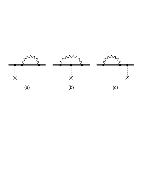
Figure 1: Feynman diagrams for the self-energy corrections to parity nonconservation. The dashed line terminated with a cross indicates an interaction with the nucleus through the exchange of a Z boson.

A principal advantage of treating the degenerate case, where the states involved in the matrix elements have the same energy, is the simplicity of the formalism. In the more general case, when the energies are different, the radiative correction to the weak interaction matrix element has to involve the laser field photon that drives the transition, otherwise one would not be dealing with a gauge-invariant amplitude. In the degenerate case we can restrict our attention to the gauge-invariant subset of diagrams shown in Fig. 1, which involve the vertex (Fig. 1b) and wave function (Figs. 1a, 1c) corrections. While the treatment of these diagrams is straightforward for scattering processes, more care is required when bound states are involved. As mentioned in the introduction, the similar problem of radiative correction to hyperfine splitting has already been treated in the literature hfsallZ ; BCS , but in the present case the initial and final states are different, and the formalism requires some modifications.

The bound state wave functions $\psi_{v}$ and $\psi_{w}$ are solutions of the Dirac equation in the field of a point nucleus. Therefore they can be interpreted as residues at poles of Dirac-Coulomb propagators as a function of energy $E\equiv p^{0}$,

$$S_{F}(\vec{r}\,^{\prime},\vec{r},E)=\Big{\langle}\vec{r}\,^{\prime}\Big{|}\frac{1}{\not\!p-m-\gamma^{0}\,V}\Big{|}\vec{r}\Big{\rangle}\approx\frac{\psi(\vec{r}\,^{\prime})\bar{\psi}(\vec{r})}{E-E_{\psi}}.$$ (8)

When radiative corrections are involved, the Dirac-Coulomb propagator is corrected by the electron self-interaction $\Sigma$

$$\Big{\langle}\vec{r}\,^{\prime}\Big{|}\frac{1}{\not\!p-m-\gamma^{0}\,V-\Sigma(E)}\Big{|}\vec{r}\Big{\rangle}.$$ (9)

The new position of the pole and corresponding residues are

$$E_{\psi}^{(1)}~{} = E_{\psi}+\langle\bar{\psi}|\Sigma(E_{\psi})|\psi\rangle$$ (10)

$$|\psi\rangle^{(1)} = |\psi\rangle+S^{\prime}_{F}(E_{\psi})\,\Sigma(E_{\psi})|\psi\rangle+\frac{|\psi\rangle}{2}\,\frac{\partial}{\partial E}\biggr{|}_{E=E_{\psi}}\!\langle\bar{\psi}|\Sigma(E)|\psi\rangle,$$ (11)

where by $S^{\prime}_{F}$ one denotes a reduced Coulomb-Dirac propagator, namely the propagator with the $\psi$-state excluded. With the help of the above equations, we now present the one-loop radiative corrections to $Q_{0}$. They consist of the vertex correction $Q_{V}$, the left and right wave function corrections $Q_{SL}+Q_{SR}$, which include as well the derivative terms, associated with the last term in Eq. (11). In the Feynman gauge they are ($\epsilon\equiv E_{v}=E_{w}$)

$$Q_{V}=-4\pi i\alpha\int\!{d^{n}k\over(2\pi)^{n}}\,{1\over k^{2}+i\delta}\,\langle w|e^{i\,\vec{k}\cdot\vec{r}}\gamma_{\mu}S_{F}(\epsilon-k_{0})\gamma_{0}\gamma_{5}\rho_{N}S_{F}(\epsilon-k_{0})\gamma^{\mu}e^{-i\,\vec{k}\cdot\vec{r}}|v\rangle,$$ (12)

$$Q_{SL} = -4\pi i\alpha\int\!{d^{n}k\over(2\pi)^{n}}\,{1\over k^{2}+i\delta}\,\langle w|\gamma_{0}\gamma_{5}\rho_{N}S^{\prime}_{F}(\epsilon)e^{i\,\vec{k}\cdot\vec{r}}\gamma_{\mu}S_{F}(\epsilon-k_{0})\gamma^{\mu}e^{-i\,\vec{k}\cdot\vec{r}}|v\rangle$$ (13)

$$+2\pi i\alpha\,Q_{0}\int\!{d^{n}k\over(2\pi)^{n}}\,{1\over k^{2}+i\delta}\,\langle w|e^{i\,\vec{k}\cdot\vec{r}}\gamma_{\mu}S_{F}(\epsilon-k_{0})\,\gamma_{0}\,S_{F}(\epsilon-k_{0})\gamma^{\mu}e^{-i\,\vec{k}\cdot\vec{r}}|w\rangle,$$

$$Q_{SR} = -4\pi i\alpha\int\!{d^{n}k\over(2\pi)^{n}}\,{1\over k^{2}+i\delta}\,\langle w|e^{i\,\vec{k}\cdot\vec{r}}\gamma_{\mu}S_{F}(\epsilon-k_{0})\gamma^{\mu}e^{-i\,\vec{k}\cdot\vec{r}}S^{\prime}_{F}(\epsilon)\gamma_{0}\gamma_{5}\rho_{N}|v\rangle$$ (14)

$$+2\pi i\alpha\,Q_{0}\int\!{d^{n}k\over(2\pi)^{n}}\,{1\over k^{2}+i\delta}\,\langle v|e^{i\,\vec{k}\cdot\vec{r}}\gamma_{\mu}S_{F}(\epsilon-k_{0})\,\gamma_{0}\,S_{F}(\epsilon-k_{0})\gamma^{\mu}e^{-i\,\vec{k}\cdot\vec{r}}|v\rangle.$$

There is still an ambiguity in the above formulas, related to the fact that at least one of the states is unstable with respect to radiative decay. This means that, for example, derivative terms, which have the interpretation of bound state wave function renormalization, acquire a small imaginary part. We think that this imaginary term may have a small effect on the weak matrix element. Nevertheless, in our treatment we completely ignore this imaginary part for simplicity. To include it properly would require a more detailed treatment of the excitation and decay process. Before the numerical integration, we present in the next section the analytic calculation of the first two terms in the $Z\alpha$ expansion.

IV $Z\alpha$ expansion

In the $Z\alpha$ expansion one performs a simplification, similar to that used for the Lamb shift, which leads to an exact expression for the expansion terms. Specifically, the first two terms are given by the on-mass-shell scattering amplitude, which because it involves the weak charge of the nucleus, is dominated by the large momentum region, with characteristic momenta of the order of the electron mass, and to smaller extent of the order of the inverse of nuclear size. The small momentum region contributes at order $O(Z\alpha)^{2}$ and will be included in the numerical treatment. We aim here to confirm the previously obtained result Milstein shown in Eq. 3, which will be used later to test the numerical accuracy of the nonperturbative treatment. In this section we do not pull out a factor $\alpha/\pi$ from $R(Z\alpha)$.

The relative correction to order ${\alpha}$ is determined by considering the radiative correction to the $\gamma^{\mu}\gamma^{5}$ vertex,

$$\Gamma^{\mu}(p_{2},p_{1})=\frac{{\alpha}}{4\pi}\int{\frac{d^{4}q}{{i}{\pi}^{2}}}\frac{N^{\mu}(p_{2},p_{1})}{[(q-k)^{2}-m^{2}+i{\epsilon}][q^{2}-m^{2}+i{\epsilon}][(q-p_{2})^{2}-{\lambda}^{2}+i{\epsilon}]},$$ (15)

where

$$N^{\mu}(p_{2},p_{1})={\gamma}^{\alpha}(\not\!q-\not\!k+m){\gamma}^{\mu}{\gamma}^{5}(\not\!q+m){\gamma}_{\alpha},$$ (16)

and $k=p_{2}-p_{1}$. The most general form of $\Gamma^{\mu}$ in momentum space is

$$\Gamma^{\mu}(p_{2},p_{1})=F_{1}(k^{2})\gamma^{\mu}{\gamma^{5}}+F_{2}(k^{2})\frac{k^{\mu}}{m}{\gamma}^{5}.$$ (17)

The form factors $F_{1}(k^{2})$ and $F_{2}(k^{2})$ are calculated following the same steps as in the case of the electromagnetic vertex. Introducing Feynman parameters and taking into account the mass-shell condition, one obtains in the limit of zero momentum transfer

$$F_{1}(0) = -\frac{\alpha}{2\pi}$$ (18)

$$F_{2}(0) = ~{}~{}\frac{7\alpha}{12\pi}.$$ (19)

For a static nucleus, only $F_{1}(0)$ contributes to the relative correction to first order in ${\alpha}$. The relative correction to the PNC amplitude is

$$R(Z\alpha)=\frac{\bar{u}(p,\sigma){\Gamma}^{0}u(p,\sigma)}{\bar{u}(p,\sigma){\gamma^{0}\gamma^{5}}{u}(p,\sigma)},$$ (20)

which can be transformed into

$$R(Z\alpha)=\frac{{\rm Tr}\Big{[}{\Gamma}^{0}\frac{1}{4m}{(\not\!p+m)}(1\,+\!\not\!a\gamma^{5})\Big{]}}{{\rm Tr}\Big{[}\gamma^{0}{\gamma}^{5}\frac{1}{4m}(\not\!p+m)(1\,+\!\not\!a\gamma^{5})\Big{]}},$$ (21)

where $a^{\mu}=(a_{0},\vec{a})$ with $a\cdot p=0$ is the polarization four vector of the electron. We then recover the well-known Marciano-Sirlin lowest-order correction

$$R(Z\alpha)=-\frac{\alpha}{2\pi}.$$ (22)

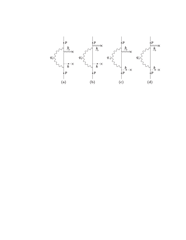
Figure 2: Feynman diagrams for the leading binding corrections to the forward scattering amplitude. The dashed and wavy lines terminated with a cross represent PNC and Coulomb interactions with the nucleus, respectively.

The leading binding correction can be derived from the forward scattering amplitude, which involves an additional Coulomb exchange. It consists of the 4 diagrams presented in Figs. 2a - 2d, which we evaluate using Yennie gauge. This gauge has the useful property that each diagram is infrared finite as the photon mass $\lambda$ is taken to 0. The contribution from Fig. 2a to the ratio $R(Z\alpha)$ can be written as

$$R_{1}=-\frac{Z\,{\alpha}^{2}}{a_{0}}\int\frac{{d^{3}k}}{(2\pi)^{3}}\frac{1}{k^{2}}\int\frac{d^{4}q}{{\pi}^{2}i}\frac{N_{1}(q,k)}{[q^{2}+i\epsilon]^{2}[(p+q)^{2}-m^{2}+i\epsilon]^{2}[(p+k+q)^{2}-m^{2}+i\epsilon]},$$ (23)

where

$$N_{1}(q,k) = (g_{\mu\nu}q^{2}+2q_{\mu}{q_{\nu}}){\rm Tr}\Big{[}\gamma^{\mu}(\not\!p\,+\!\not\!q+m){\gamma}^{0}(\not\!p\,+\!\not\!q\,+\!\not\!k+m){\gamma^{0}{\gamma}^{5}}$$ (24)

$$\times(\not\!p\,+\!\not\!q+m){\gamma}^{\nu}\frac{1}{4m}{(\not\!p+m)}{(1\,+\!\not\!a{\gamma}^{5})}\Big{]}.$$

For Figs. 2b and 2c, we have

$$R_{i} = -\frac{Z\,{\alpha}^{2}}{a_{0}}\int\frac{{d^{3}k}}{(2\pi)^{3}}\frac{1}{k^{2}}\int\frac{d^{4}q}{{\pi}^{2}i}\frac{1}{[q^{2}+i\epsilon]^{2}}$$ (25)

$$\times\frac{N_{i}(q,k)}{[(p+q)^{2}-m^{2}+i\epsilon][(p+k+q)^{2}-m^{2}+i\epsilon][(p+k)^{2}-m^{2}+i{\epsilon}]},$$

where

$$N_{2}(q,k) = (g_{\mu\nu}q^{2}+2q_{\mu}{q_{\nu}}){\rm Tr}\Big{[}{\gamma}^{0}(\not\!p\,+\!\not\!k+m){\gamma}^{\mu}(\not\!p\,+\!\not\!k\,+\!\not\!q+m){\gamma}^{0}\gamma^{5}$$ (26)

$$\times(\not\!p\,+\!\not\!q+m){\gamma}^{\nu}\frac{1}{4m}{(\not\!p+m)}{(1\,+\!\not\!a{\gamma}^{5})}\Big{]},$$

$$N_{3}(q,k) = (g_{\mu\nu}q^{2}+2q_{\mu}{q_{\nu}}){\rm Tr}\Big{[}{\gamma}^{\mu}(\not\!p\,+\!\not\!q+m){\gamma}^{0}(\not\!p\,+\!\not\!k\,+\!\not\!q+m){\gamma}^{\nu}$$ (27)

$$\times(\not\!p\,+\!\not\!k+m)\gamma^{0}\gamma^{5}{\frac{1}{4m}}(\not\!p+m){(1\,+\!\not\!a{\gamma}^{5})}\Big{]}.$$

Finally, for Fig. 2d, one has

$$R_{4}=-\frac{Z\,{\alpha}^{2}}{a_{0}}\int\frac{{d^{3}k}}{(2\pi)^{3}}\frac{1}{k^{2}}\int\frac{d^{4}q}{{\pi}^{2}i}\frac{N_{4}(q,k)}{[q^{2}+i\epsilon]^{2}[(p+k)^{2}-m^{2}+i\epsilon]^{2}[(p+k+q)^{2}-m^{2}+i\epsilon]}$$ (28)

$$N_{4}(q,k) = (g_{\mu\nu}q^{2}+2q_{\mu}{q_{\nu}}){\rm Tr}\Big{[}{\gamma}^{0}(\not\!p\,+\!\not\!k+m){\gamma}^{\mu}(\not\!p\,+\!\not\!q+m){\gamma}^{\nu}(\not\!p\,+\!\not\!k+m){\gamma}^{0}$$ (29)

$$\times{\gamma}^{5}{\frac{1}{4m}}(\not\!p+m){(1\,+\!\not\!a{\gamma}^{5})}\Big{]},$$

where $k=(0,\vec{k})$. Each contribution from Figs. 2a, 2b, 2c and 2d is written as

$$-\frac{Z\,{\alpha}^{2}}{a_{0}}\!\int\!\frac{d^{3}k}{{(2\pi)}^{3}}\frac{F_{i}(k^{2})}{k^{2}}.$$ (30)

The calculations are considerably simplified if one determines only the imaginary part of the functions $F_{i}(k^{2})$. These are analytic functions with a branch cut for $k^{2}>0$. The real part of $F_{i}(k^{2})$ is then obtained by means of Cauchy’s theorem,

$$F(k^{2})=\frac{1}{2\pi i}\int dM^{2}\frac{F(M^{2}+i0)-F(M^{2}-i0)}{M^{2}-k^{2}}=\frac{1}{\pi}\int dM^{2}{\frac{{\Im[F(M^{2})]}}{M^{2}-k^{2}}},$$ (31)

where $k^{2}<0$. Substituting this expression into Eq. (30) and integrating over $k$ yields

$${R_{i}}=\frac{Z\,{\alpha}^{2}}{2{\pi}^{2}a_{0}}{\int}^{\infty}_{0}{dM}\Im[F_{i}(M^{2})].$$ (32)

In order to calculate $\Im[F_{i}]$, a procedure in Mathematica is written which facilitates the evaluation of the trace in Eq. (24) and the the integrals in Eq. (32). Each contribution is doubled due to the permutation of photon and boson lines. Setting $m=1$ and picking the terms linear in ${\vec{p}}$, we obtain

$$\sum_{i=1}^{4}\Im[F_{i}(M^{2})]=2a_{0}\pi\biggl{\{}\frac{7}{3}-\frac{32}{3M^{2}}+\frac{2}{3(1+M^{2})^{2}}-\frac{1}{1+M^{2}}+2\,\biggl{(}\frac{16}{3M^{3}}-\frac{1}{M}-\frac{M}{6}\biggr{)}$$

$$\times\biggl{[}\arctan(M)-\arccos\Bigl{(}\frac{2}{M}\Bigr{)}\theta(M-2)\biggr{]}-2\,\biggl{(}1-\frac{10}{3M^{2}}\biggr{)}\sqrt{1-\frac{4}{M^{2}}}\,\theta(M-2)\biggr{\}},$$ (33)

where $\theta$ is the step function with $\theta(x)=0$ for $x<0$ and $\theta(x)=1$ for $x>0$. The above expression can be analytically integrated. Hence we have

$$R(Z\alpha)\;=\;-\frac{\alpha}{2\pi}+\sum_{i=1}^{4}R_{i}\;=\;-\frac{\alpha}{2\pi}+\frac{Z\alpha^{2}}{2{\pi}^{2}a_{0}}\int_{0}^{\infty}\!dM\sum_{i=1}^{4}\Im[F_{i}]\;=\;-\frac{\alpha}{2\pi}-\biggl{(}\frac{7}{12}+2{\rm ln}2\biggr{)}Z\alpha^{2},$$ (34)

in agreement with Ref. Milstein . We now turn to the numerical calculation.

V Numerical approach

In order to make contact with the notation used in Ref. BCS , we note that the two terms $Q_{SL}$ and $Q_{SR}$ in Eqs. (13) and (14) are associated with what are called “side-left” (SL) and “side-right” (SR) diagrams in that work, which notation we will follow in this section. In addition, the SL and SR diagrams have contributions called “derivative terms”. We will refer in this section to the Gell-Mann Low formalism used in Ref. BCS in a rederivation of Eqs. (13) and (14): the adiabatic damping factor $\epsilon$ used in that formalism can be distinguished from the factor used in dimensional regularization, $n=4-\epsilon$, by context. In the numerical evaluation, each diagram breaks into several pieces, which we define as

$$Q=\sum_{i=1}^{3}Q_{Vi}+\sum_{i=1}^{4}Q_{SLi}+\sum_{i=1}^{4}Q_{SRi}.$$ (35)

We now treat the vertex and side diagrams in turn.

V.1 Vertex diagram

The vertex diagram $Q_{V}$, shown in Fig. 1b, was given in Eq. (12). The ultraviolet divergent part of the diagram can be isolated by replacing $S_{F}$ with $S_{0}$, where $S_{0}$ is a free propagator. If this replacement is made, we get the contribution $Q_{V1}$ which is most conveniently evaluated in momentum space

$$Q_{V1}=-4\pi i\alpha\int\!\frac{d^{3}p_{2}}{(2\pi)^{3}}\,\frac{d^{3}p_{1}}{(2\pi)^{3}}\int\!{d^{n}k\over(2\pi)^{n}}\,{1\over k^{2}+i\delta}\,\bar{\psi}_{w}(\vec{p}_{2})\gamma_{\mu}{1\over\not\!p_{2}\,-\!\not\!k-m}V(q){1\over\not\!p_{1}\,-\!\not\!k-m}\gamma^{\mu}\psi_{v}(\vec{p}_{1}).$$ (36)

After Feynman parameterization the $d^{n}k$ integration can be carried out with the result

$$Q_{V1} = {\alpha\over 2\pi}\biggl{(}{C\over\epsilon}-1\biggr{)}Q_{0}-{\alpha\over 2\pi}\int_{0}^{1}\!\rho d\rho\int_{0}^{1}\!dx\!\int\!\frac{d^{3}p_{2}}{(2\,\pi)^{3}}\,\frac{d^{3}p_{1}}{(2\,\pi)^{3}}\,\bar{\psi}_{w}(\vec{p}_{2})V(q)\psi_{v}(\vec{p}_{1})\,{\rm ln}{\Delta_{V}\over m^{2}}$$ (37)

$$-\,{\alpha\over 4\pi}\int_{0}^{1}\!\rho d\rho\int_{0}^{1}\!dx\!\int\!\frac{d^{3}p_{2}}{(2\,\pi)^{3}}\,\frac{d^{3}p_{1}}{(2\,\pi)^{3}}$$

$$\times\Big{[}\bar{\psi}_{w}(\vec{p}_{2})\gamma_{\mu}(\not\!p_{2}-\not\!Q+m)V(q)(\not\!p_{1}-\not\!Q+m)\gamma^{\mu}\psi_{v}(\vec{p}_{1})\Big{]}{1\over\Delta_{V}}.$$

Here

$$C~{} = (4\pi)^{\epsilon/2}\Gamma(1+\epsilon/2),$$

$$Q_{\mu} = \rho\,x\,{p_{1}}_{\mu}+\rho(1-x){p_{2}}_{\mu},$$

$$\Delta_{V} = \rho x(m^{2}-p_{1}^{2})+\rho(1-x)(m^{2}-p_{2}^{2})+Q^{2},$$

$$q~{} = |\vec{p}_{2}-\vec{p}_{1}|,$$

and the Fourier transform of the weak Hamiltonian in the case of a uniform charge distribution is

$$V(q)={3\over 8\pi^{3}(qR_{0})^{3}}\Big{[}{\rm sin}(qR_{0})-qR_{0}{\rm cos}(qR_{0})\Big{]}\gamma_{0}\gamma_{5}.$$ (38)

The first two terms in the right-hand-side of Eq. (37) are divergent and will be held for later cancellation with the “derivative terms” from the SL and SR calculation. The remaining finite parts of $Q_{V1}$ are tabulated in the second column of Table 2.

The difference of $Q_{V}$ and $Q_{V1}$ is ultraviolet finite, and is evaluated in coordinate space. The $k_{0}$ integral is treated by carrying out a Wick rotation, $k_{0}\rightarrow i\omega$, which leads to

$$Q_{V2} = -8\pi\alpha\,\Re\!\int\!d^{3}x\!\int\!d^{3}y\!\int\!d^{3}z\int_{0}^{\infty}{d\omega\over 2\pi}\int\!{d^{3}k\over(2\pi)^{3}}\,{e^{i\vec{k}\cdot(\vec{x}-\vec{z})}\over\omega^{2}+\vec{k}^{2}}$$ (39)

$$\times\Bigr{[}\bar{\psi}_{w}(\vec{x})\gamma_{\mu}S_{F}(\vec{x},\vec{y},\epsilon_{w}-i\omega)\gamma_{0}\gamma_{5}\rho_{N}(\vec{y})S_{F}(\vec{y},\vec{z};\epsilon_{v}-i\omega)\gamma^{\mu}\psi_{v}(\vec{z})$$

$$-\,\bar{\psi}_{w}(\vec{x})\gamma_{\mu}S_{0}(\vec{x},\vec{y},\epsilon_{w}-i\omega)\gamma_{0}\gamma_{5}\rho_{N}(\vec{y})S_{0}(\vec{y},\vec{z};\epsilon_{v}-i\omega)\gamma^{\mu}\psi_{v}(\vec{z})\Bigr{]}.$$

A singularity associated with the parts of the bound propagators which include $w$ or $v$ is regularized by evaluating the expression with $\epsilon_{w,v}\rightarrow\epsilon_{w,v}(1-\Delta)$ in the electron propagators. The result behaves as ln$\Delta$. While it is possible to explicitly cancel this dependence with similar terms from the side diagrams, we choose here to simply work with a specific, small value of $\Delta=10^{-5}$. We note that different choices of $\Delta$ will lead to slightly different results for $Q_{V2}$, but when combined with the side diagrams discussed below, the sums are essentially the same as long as the values of $\Delta$ are reasonably small. Results for $Q_{V2}$ with $\Delta=10^{-5}$ are given in the third column of Table 2.

The Wick rotation mentioned above passes bound state poles which must be accounted for. They are treated by rewriting $Q_{V}$ by treating the propagators as a spectral representation, carrying out the $d^{3}k$ integration analytically, and defining

$$g_{ijkl}(E)\equiv\alpha\int\!d^{3}x\,d^{3}y\,{e^{i\sqrt{E^{2}+i\delta}\,|\vec{x}-\vec{y}\,|}\over|\vec{x}-\vec{y}\,|}\,\bar{\psi}_{i}(\vec{x})\gamma_{\mu}\psi_{k}(\vec{x})\,\bar{\psi}_{j}(\vec{y})\gamma^{\mu}\psi_{l}(\vec{y}),$$ (40)

which allows us to write

$$Q_{V}=i\int{dk_{0}\over 2\pi}\sum_{mn}{g_{wnmv}(k_{0})Q_{mn}\over[\epsilon_{w}(1-\Delta)-k_{0}-\epsilon_{m}(1-i\delta)][\epsilon_{v}(1-\Delta)-k_{0}-\epsilon_{n}(1-i\delta)]}.$$ (41)

The choice we have made in regularizing leads to only the ground state $1s_{1/2}$, denoted as $a$, being encircled when $k_{0}\rightarrow i\omega$, so

$$Q_{V3}=\sum_{an}{g_{wnav}(\epsilon_{w}-\epsilon_{a})Q_{an}\over\epsilon_{a}-\epsilon_{n}}+\sum_{ma}{g_{wamv}(\epsilon_{v}-\epsilon_{a})Q_{ma}\over\epsilon_{a}-\epsilon_{m}}.$$ (42)

The sum over $a$ ranges only over the two magnetic quantum numbers of the state. This contribution is tabulated in the fourth column of Table 2. The part of the summation in which the denominator would vanish corresponds to a double pole, but does not contribute because $Q_{aa}$ vanishes. However, it should be noted that double poles will in general contribute, and in fact would be present in the present calculation were we to use a negative value of $\Delta$ which would introduce additional pole terms from the $2s_{1/2}$ and $2p_{1/2}$ states.

V.2 Side diagrams

It is convenient for the discussion of the side diagrams to introduce the matrix element of the self-energy operator between two arbitrary states $m$ and $n$,

$$\Sigma_{mn}(E)=-ie^{2}\!\int\!d^{3}xd^{3}y\!\int\!{d^{n}k\over(2\pi)^{n}}\,{e^{i\vec{k}\cdot(\vec{x}-\vec{y})}\over k^{2}+i\delta}\,\bar{\psi}_{m}(\vec{x})\gamma_{\mu}S_{F}(\vec{x},\vec{y};E-k_{0})\gamma^{\mu}\psi_{n}(\vec{y}).$$ (43)

A self-mass counterterm is understood to be included in the above. The self-energy of a valence state is then $\Sigma_{vv}(\epsilon_{v})$, and can be evaluated as described in Ref. CJS .

Using a spectral decomposition of the intermediate propagator, the $S$-matrix for SL is

$$Q_{SL}=-i\lambda^{3}\sum_{m}\int{dE_{1}\over 2\pi}\int{dE_{2}\over 2\pi}{Q_{wm}\Sigma_{mv}(E_{2})\over E_{1}-\epsilon_{m}(1-i\delta)}\Delta(E_{1}-\epsilon_{w})\Delta(E_{1}-E_{2}-k_{0})\Delta(E_{2}+k_{0}-\epsilon_{v}),$$ (44)

and for SR

$$Q_{SR}=-i\lambda^{3}\sum_{m}\int{dE_{1}\over 2\pi}\int{dE_{2}\over 2\pi}{\Sigma_{wm}(E_{1})Q_{mv}\over E_{2}-\epsilon_{m}(1-i\delta)}\Delta(E_{2}-\epsilon_{v})\Delta(E_{1}-E_{2}+k_{0})\Delta(E_{1}+k_{0}-\epsilon_{w}),$$ (45)

with

$$\Delta(E)={2\epsilon\over E^{2}+\epsilon^{2}}.$$ (46)

Here $\lambda$ is a factor associated with the Gell-Mann-Low formalism GML that is to be differentiated and set to unity: in addition, a factor $i\epsilon/2$ must be multiplied into the $S$-matrix to obtain the off-diagonal energy. If the restriction is made that $m\neq w,v$, it is straightforward to show that two “perturbed orbital” (PO) contributions to the matrix element result which are given by

$$Q_{SL1}=\sum_{m\neq v}{Q_{wm}\Sigma_{mv}(\epsilon_{v})\over\epsilon_{w}-\epsilon_{m}}\equiv\Sigma_{\tilde{v}v}(\epsilon_{v})$$ (47)

and

$$Q_{SR1}=\sum_{m\neq w}{\Sigma_{wm}(\epsilon_{w})Q_{mv}\over\epsilon_{v}-\epsilon_{m}}\equiv\Sigma_{w\tilde{w}}(\epsilon_{w}).$$ (48)

This is equivalent to the forms given for $Q_{SL}$ and $Q_{SR}$ in Eqs. (13) and (14). We note that it is not necessary to explicitly make the restrictions $m\neq w$ in $Q_{SL1}$ and $m\neq v$ in $Q_{SR1}$ because $Q_{ww}=Q_{vv}=0$. The PO terminology arises from the fact that the $m$ summation can be carried out before evaluating the self-energy, and one then needs only to do a self-energy calculation with one of the external wavefunctions replaced with a perturbed orbital. The PO terms are tabulated in the fifth and ninth columns of Table 2.

The cases $m=v$ and $m=w$ are more subtle, as they contribute terms of order $1/\epsilon$ to the off-diagonal energy. This divergence cancels, but a finite contribution coming from Taylor expanding $\Sigma(E)$ remains, and contributes ${1\over 2}Q_{0}{\Sigma}^{\prime}_{vv}(\epsilon_{v})+{1\over 2}Q_{0}{\Sigma}^{\prime}_{ww}(\epsilon_{w})$, or more explicitly

$$Q^{\rm der}_{SL} = 2i\pi\alpha Q_{0}\int d^{3}yd^{3}zd^{3}w\int{d^{n}k\over(2\pi)^{n}}{e^{i\vec{k}\cdot(\vec{y}-\vec{z})}\over k^{2}+i\delta}$$ (49)

$$\times\bar{\psi}_{v}(\vec{y})\gamma_{\mu}S_{F}(\vec{y},\vec{w};\epsilon_{v}-k_{0})\gamma_{0}S_{F}(\vec{w},\vec{z};\epsilon_{v}-k_{0})\gamma^{\mu}\psi_{v}(\vec{z})$$

$$= -{i\over 2}Q_{0}\sum_{m}\int{dk_{0}\over 2\pi}{g_{vmmv}(k_{0})\over(\epsilon_{v}-k_{0}-\epsilon_{m})^{2}}$$

and

$$Q^{\rm der}_{SR} = 2i\pi\alpha Q_{0}\int d^{3}yd^{3}zd^{3}w\int{d^{n}k\over(2\pi)^{n}}{e^{i\vec{k}\cdot(\vec{y}-\vec{z})}\over k^{2}+i\delta}$$ (50)

$$\times\bar{\psi}_{w}\gamma_{\mu}S_{F}(\vec{y},\vec{w};\epsilon_{w}-k_{0})\gamma_{0}S_{F}(\vec{w},\vec{z};\epsilon_{w}-k_{0})\gamma^{\mu}\psi_{w}(\vec{z})$$

$$= -{i\over 2}Q_{0}\sum_{m}\int{dk_{0}\over 2\pi}{g_{wmmw}(k_{0})\over(\epsilon_{w}-k_{0}-\epsilon_{m})^{2}}.$$

These correspond to the derivative term mentioned in the preceding section. The analysis of this term parallels closely the treatment of the vertex: first the bound propagators are replaced with free propagators, which gives

$$Q_{SL2}=2\pi i\alpha Q_{0}\!\int\!\frac{d^{3}p}{(2\,\pi)^{3}}\!\int\!{d^{n}k\over(2\pi)^{n}}\,\bar{\psi}_{v}(\vec{p})\gamma_{\mu}{1\over\not\!p\,-\!\not\!k-m}\gamma_{0}{1\over\not\!p\,-\!\not\!k-m}\gamma^{\mu}\psi_{v}(\vec{p})$$ (51)

and

$$Q_{SR2}=2\pi i\alpha Q_{0}\!\int\!\frac{d^{3}p}{(2\,\pi)^{3}}\!\int\!{d^{n}k\over(2\pi)^{n}}\,\bar{\psi}_{w}(\vec{p})\gamma_{\mu}{1\over\not\!p\,-\!\not\!k-m}\gamma_{0}{1\over\not\!p\,-\!\not\!k-m}\gamma^{\mu}\psi_{w}(\vec{p}).$$ (52)

Feynman parameterizing and carrying out the $d^{n}k$ integration gives

$$Q_{SL2} = -{\alpha\over 4\pi}\biggl{(}{C\over\epsilon}-1\biggr{)}Q_{0}+{\alpha\over 4\pi}Q_{0}\int_{0}^{1}\!\rho d\rho\int\!\frac{d^{3}p}{(2\,\pi)^{3}}\,\bar{\psi}_{v}(\vec{p})\gamma_{0}\psi_{v}(\vec{p}){\rm ln}{\Delta_{S}\over m^{2}}$$ (53)

$$+{\alpha\over 8\pi}Q_{0}\int_{0}^{1}\!\rho d\rho\!\int\!\frac{d^{3}p}{(2\,\pi)^{3}}\Big{\{}\bar{\psi}_{v}(\vec{p})\gamma_{\mu}\big{[}\!\not\!p(1-\rho)+m\big{]}\gamma_{0}\big{[}\!\not\!p(1-\rho)+m\big{]}\gamma^{\mu}\psi_{v}(\vec{p})\Big{\}}{1\over\Delta_{S}}.$$

and

$$Q_{SR2} = -{\alpha\over 4\pi}\biggl{(}{C\over\epsilon}-1\biggr{)}Q_{0}+{\alpha\over 4\pi}Q_{0}\int_{0}^{1}\!\rho d\rho\int\!\frac{d^{3}p}{(2\,\pi)^{3}}\,\bar{\psi}_{w}(\vec{p})\gamma_{0}\psi_{w}(\vec{p}){\rm ln}{\Delta_{S}\over m^{2}}$$ (54)

$$+{\alpha\over 8\pi}Q_{0}\int_{0}^{1}\!\rho d\rho\!\int\!\frac{d^{3}p}{(2\,\pi)^{3}}\Big{\{}\bar{\psi}_{w}(\vec{p})\gamma_{\mu}\big{[}\!\not\!p(1-\rho)+m\big{]}\gamma_{0}\big{[}\!\not\!p(1-\rho)+m\big{]}\gamma^{\mu}\psi_{w}(\vec{p})\Big{\}}{1\over\Delta_{S}}.$$

where $\Delta_{S}=\rho^{2}p^{2}+\rho(m^{2}-p^{2})$. The first two terms in the right-hand-side of the above equations for $Q_{SL2}$ and $Q_{SR2}$ are divergent but cancel with the corresponding terms of $Q_{V1}$ in Eq. (37). The remaining, finite terms are presented in the sixth and tenth columns of Table 2.

The difference of the side diagrams evaluated with bound propagators and free propagators is again ultraviolet finite, and after Wick rotation one has

$$Q_{SL3} = 2\pi Q_{0}\alpha\,\Re\!\int\!d^{3}x\!\int\!d^{3}y\!\int\!d^{3}z\!\int\!{d\omega\over 2\pi}\!\int\!{d^{3}k\over(2\pi)^{3}}\,{e^{i\vec{k}\cdot(\vec{x}-\vec{z})}\over\omega^{2}+\vec{k}^{2}}$$ (55)

$$\times\biggl{[}\bar{\psi}_{v}(\vec{x})\gamma_{\mu}S_{F}(\vec{x},\vec{y},\epsilon_{v}-i\omega)\gamma_{0}S_{F}(\vec{y},\vec{z};\epsilon_{v}-i\omega)\gamma^{\mu}\psi_{v}(\vec{z})$$

$$-\,\bar{\psi}_{v}(\vec{x})\gamma_{\mu}S_{0}(\vec{x},\vec{y},\epsilon_{v}-i\omega)\gamma_{0}S_{0}(\vec{y},\vec{z};\epsilon_{v}-i\omega)\gamma^{\mu}\psi_{v}(\vec{z})\biggr{]}.$$

and

$$Q_{SR3} = 2\pi Q_{0}\alpha\,\Re\!\int\!d^{3}x\!\int\!d^{3}y\!\int\!d^{3}z\!\int\!{d\omega\over 2\pi}\!\int\!{d^{3}k\over(2\pi)^{3}}\,{e^{i\vec{k}\cdot(\vec{x}-\vec{z})}\over\omega^{2}+\vec{k}^{2}}$$ (56)

$$\times\biggl{[}\bar{\psi}_{w}(\vec{x})\gamma_{\mu}S_{F}(\vec{x},\vec{y},\epsilon_{w}-i\omega)\gamma_{0}S_{F}(\vec{y},\vec{z};\epsilon_{w}-i\omega)\gamma^{\mu}\psi_{w}(\vec{z})$$

$$-\,\bar{\psi}_{w}(\vec{x})\gamma_{\mu}S_{0}(\vec{x},\vec{y},\epsilon_{w}-i\omega)\gamma_{0}S_{0}(\vec{y},\vec{z};\epsilon_{w}-i\omega)\gamma^{\mu}\psi_{w}(\vec{z})\biggr{]}.$$

The same regularization of the valence energy, $\epsilon_{v}\rightarrow\epsilon_{v}(1-\Delta)$ used in the vertex is required, and again we simply use $\Delta=10^{-5}$ and present the results in the seventh and eleventh columns of Table 2.

Finally, the Wick rotation passes a double pole when $m=a$, with $a$ being the $1s_{1/2}$ ground state, leading to the derivative terms

$$Q_{SL4}={1\over 2}Q_{0}\sum_{a}g^{\prime}_{vaav}(\epsilon_{v}-\epsilon_{a})$$ (57)

and

$$Q_{SR4}={1\over 2}Q_{0}\sum_{a}g^{\prime}_{waaw}(\epsilon_{w}-\epsilon_{a})$$ (58)

which are tabulated in the eighth and twelfth column of Table 2. This completes the calculation and the sums of vertex and side diagram contributions give the values of the exact evaluation of the function $R(Z\alpha)$ which are tabulated in the last column of Table 2.

VI discussion

A number of numerical issues arise in the calculation that we note here. In some parts the use of a uniform distribution, with its step function behavior, caused loss of accuracy. In those cases a fermi distribution was used: while this leads to small changes in $Q_{0}$, the effect on $R(Z\alpha)$ is negligible. More serious is the difficulty of controlling numerical instabilities at low $Z$, which led to our choosing the lowest $Z$ to be 10. A graph of the numerical value of $R(Z\alpha)$, along with results from the two leading terms given in Eq. 3, is shown in Fig. 3. The accuracy of the calculation at low $Z$ is sufficient to allow a fit that determines

$$R(Z\alpha)_{\rm fit}=-{1\over 2}-0.045(2)Z.$$ (59)

which is in agreement with the numerical value of Eq. (3)

$$R(Z\alpha)=-{1\over 2}-0.045154Z.$$ (60)

This agreement provides a check on the rather complex numerical calculation. The advantage of the numerical approach is of course the fact that it does not assume $Z\alpha$ to be a small parameter, and thus can be used for high $Z$. In the particularly interesting case of $Z=55$, we see that the perturbative formula happens to be -2.983, as compared with the exact result -4.007.

However, at this point we make no claims about the applicability of the present calculation to the case of PNC transitions in neutral cesium. The actual process studied in the experiment that measures PNC Wieman involves a double perturbation, where not only the weak Hamiltonian but also an external laser photon field act to either first transform the $6s_{1/2}$ electron into a state with the opposite parity, followed by an allowed dipole transition to a $7s_{1/2}$ electron, or vice-versa. To extend our calculation to the actual experiment requires the following steps.

The first step is replacing the Coulomb wave functions used here with realistic wave functions for neutral cesium. The technology to carry out radiative corrections in neutral atoms has only recently been put into place. It is now possible, using a local potential that incorporates screening, to carry out accurate self-energy Pyykko ; CS and radiative correction to hfs NewCS calculations. The second step is to incorporate the laser photon. This is a more complicated task, since the set of diagrams shown in Fig. 4 must be evaluated. We note that while Fig. 4a corresponds to the vertex correction considered here, Fig. 4c corresponds to a radiative correction to the electromagnetic vertex, and Fig. 4e to a new radiative correction specific to the experiment. We expect that the new contributions will affect $R(Z\alpha)$ in order $(Z\alpha)^{2}$, but until they are explicitly evaluated, their importance for cesium PNC is unknown.

The principal results of this paper are then as follows. Firstly, an independent scattering calculation of the leading binding correction in the function $R(Z\alpha)$ has been presented, which confirms the calculation of Ref. Milstein . Secondly, it has been shown that numerical methods that allow the evaluation of $R(Z\alpha)$ to all orders in $Z\alpha$ for the case of gauge-invariant $2s_{1/2}-2p_{1/2}$ transitions in hydrogenlike ions can be applied. The behavior of the function shows that large binding corrections are present. If these corrections behave the same in the realistic cesium case, and the extra corrections of order $(Z\alpha)^{2}$ mentioned above are small, the apparent $2\sigma$ discrepancy noted in Ref. vacpol is reduced, but before a complete calculation is completed the theoretical status of PNC in cesium should be regarded as unresolved.

Figure 3: Comparison of exact calculation (solid line) with first two terms of perturbative expansion for $R(Z\alpha)$ (dashed line).

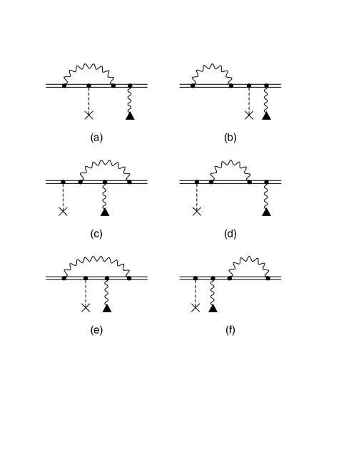
Figure 4: Feynman diagrams for the radiative correction to electron excitation by a laser photon, indicated by the wavy line terminated with a triangle, in the presence of interaction with the nucleus through exchange of a Z boson, indicated by the dashed line terminated with a cross.

Table 1: Nuclear parameters $c$ and $R_{0}$ and lowest-order PNC matrix element $Q_{0}$: units of fermis for $c$ and $R_{0}$ and $1/a_{0}^{3}$ for $Q_{0}$. Square brackets indicate power of 10.

$Z$	$c$	$R_{0}$	$Q_{0}$
10	2.9889	3.859	1.318[0]
15	3.2752	4.127	7.038[0]
20	3.7188	4.487	2.388[1]
25	4.0706	4.783	6.366[1]
30	4.4454	5.106	1.465[2]
40	4.9115	5.516	5.988[2]
50	5.4595	6.010	2.010[3]
55	5.6748	6.206	3.539[3]
60	5.8270	6.345	6.136[3]
70	6.2771	6.761	1.786[4]
80	6.6069	7.068	5.184[4]
90	6.9264	7.368	1.542[5]
100	7.1717	7.599	4.886[5]

Table 2: Breakdown of Contributions to $R(Z\alpha)$.

$Z$	$Q_{V1}$	$Q_{V2}$	$Q_{V3}$	$Q_{SL1}$	$Q_{SL2}$	$Q_{SL3}$	$Q_{SL4}$	$Q_{SR1}$	$Q_{SR2}$	$Q_{SR3}$	$Q_{SR4}$	$R(Z\alpha)$
10	-2.500	4.260	-11.768	-0.272	2.369	2.293	0.002	-0.045	2.269	2.388	0.006	-0.998
15	-2.009	-0.253	-7.853	-0.415	1.972	2.689	0.003	-0.068	1.873	2.782	0.009	-1.270
20	-1.729	-2.600	-5.898	-0.555	1.694	2.967	0.004	-0.097	1.595	3.058	0.012	-1.549
25	-1.559	-4.064	-4.727	-0.696	1.482	3.180	0.005	-0.128	1.384	3.269	0.014	-1.840
30	-1.458	-5.067	-3.948	-0.839	1.311	3.350	0.006	-0.164	1.214	3.439	0.017	-2.139
40	-1.377	-6.398	-2.980	-1.139	1.048	3.620	0.008	-0.279	0.952	3.703	0.022	-2.820
50	-1.386	-7.267	-2.406	-1.461	0.851	3.824	0.011	-0.434	0.755	3.904	0.026	-3.583
55	-1.411	-7.609	-2.201	-1.637	0.768	3.911	0.012	-0.530	0.673	3.989	0.028	-4.007
60	-1.446	-7.912	-2.033	-1.821	0.694	3.990	0.013	-0.644	0.600	4.067	0.030	-4.462
70	-1.525	-8.466	-1.778	-2.229	0.566	4.132	0.016	-0.922	0.472	4.207	0.033	-5.494
80	-1.617	-8.922	-1.602	-2.707	0.458	4.253	0.019	-1.300	0.365	4.331	0.035	-6.687
90	-1.708	-9.376	-1.489	-3.288	0.364	4.366	0.023	-1.822	0.273	4.448	0.035	-8.174
100	-1.798	-9.831	-1.433	-4.020	0.282	4.457	0.028	-2.570	0.192	4.545	0.033	-10.115