KA-TP-03-2003
MPI-PhT/2003-08
PSI-PR-03-05
hep-ph/0302198

Electroweak radiative corrections to ${\mathrm{e^{+}}}{\mathrm{e^{-}}}\to\nu\bar{\nu}{\mathrm{H}}$

A. Denner¹, S. Dittmaier², M. Roth³ and M. M. Weber¹

¹ Paul-Scherrer-Institut, Würenlingen und Villigen
CH-5232 Villigen PSI, Switzerland

² Max-Planck-Institut für Physik (Werner-Heisenberg-Institut)
D-80805 München, Germany

³ Institut für Theoretische Physik, Universität Karlsruhe
D-76128 Karslruhe, Germany

Abstract:

The complete electroweak ${\cal O}(\alpha)$ radiative corrections to the Higgs-boson production processes ${\mathrm{e^{+}}}{\mathrm{e^{-}}}\to\nu_{l}\bar{\nu}_{l}{\mathrm{H}}$ ($l={\mathrm{e}},\mu,\tau$) are calculated in the electroweak Standard Model. For ${\mathrm{e^{+}}}{\mathrm{e^{-}}}\to\nu_{\mathrm{e}}\bar{\nu}_{\mathrm{e}}{\mathrm{H}}$, where ${\mathrm{Z}}{\mathrm{H}}$ production and W-boson fusion contribute, both production channels are added coherently. The calculation of the corrections is described in some detail including, in particular, the treatment of the Z-boson resonance in the ${\mathrm{Z}}{\mathrm{H}}$-production channel. The discussion of numerical results focusses on the total cross section as well as on angular and energy distributions of the Higgs boson. In the $G_{\mu}$-scheme, the bulk of the corrections is due to initial-state radiation. The corrections turn out to reduce the total cross section by $\sim 10\%$ for high energies, where the W-boson fusion dominates. In this region, the corrections depend only weakly on the energy and the production angle of the Higgs boson. Based on an analysis of the leading universal corrections, a simple improved Born approximation is introduced. This approximation describes the corrected cross section within about 3%.

February 2003

1 Introduction

One of the most important open problems of particle physics is the understanding of the mechanism of electroweak symmetry breaking. In the electroweak Standard Model (SM) it is provided by the Higgs mechanism, leading to the prediction of a physical scalar particle, the Higgs boson. The investigation of the mechanism of electroweak symmetry breaking and, in particular, of the Higgs boson, will be one of the main concerns at the Large Hadron Collider (LHC) at CERN. The LHC experiments ATLAS [1] and CMS [2] are sensitive to the SM Higgs boson over the whole mass range from the present lower experimental limit of $114.4\,\mathrm{GeV}$ [3] up to $1\,\mathrm{TeV}$ and will discover the Higgs boson, if it exists and has no particularly exotic properties. Moreover, these experiments will determine various properties of the Higgs boson, such as its mass, branching ratios, and ratios of its coupling constants.

However, the complete profile of the Higgs boson can only be studied in the clean environment of an electron–positron linear collider [4, 5, 6, 7]. In ${\mathrm{e^{+}}}{\mathrm{e^{-}}}$ annihilation there are two main production mechanisms for the SM Higgs boson. In the Higgs-strahlung process, ${\mathrm{e^{+}}}{\mathrm{e^{-}}}\to{\mathrm{Z}}{\mathrm{H}}$, a virtual ${\mathrm{Z}}$ boson decays into a ${\mathrm{Z}}$ boson and a Higgs boson. The corresponding cross section rises sharply at threshold to a maximum of a few tens of GeV above $M_{\mathrm{Z}}+M_{\mathrm{H}}$ and then falls off as $s^{-1}$, where $\sqrt{s}$ is the centre-of-mass (CM) energy of the ${\mathrm{e^{+}}}{\mathrm{e^{-}}}$ system. In the W-boson-fusion process, ${\mathrm{e^{+}}}{\mathrm{e^{-}}}\to\nu_{\mathrm{e}}\bar{\nu}_{\mathrm{e}}{\mathrm{H}}$, the incoming ${\mathrm{e^{+}}}$ and ${\mathrm{e^{-}}}$ each emit a virtual W boson which fuse into a Higgs boson. The cross section of the W-boson-fusion process grows as $\ln s$ and thus is the dominant production mechanism for $\sqrt{s}\gg M_{\mathrm{H}}$. The cross section for the similar ${\mathrm{Z}}$-boson-fusion process, ${\mathrm{e^{+}}}{\mathrm{e^{-}}}\to{\mathrm{e^{+}}}{\mathrm{e^{-}}}{\mathrm{H}}$, is about one order of magnitude smaller.

At a linear ${\mathrm{e^{+}}}{\mathrm{e^{-}}}$ collider with a CM energy of $500\,\mathrm{GeV}$ and an integrated luminosity of $500\,\mathrm{fb}^{-1}$, of the order of $10^{4}$ Higgs bosons can be produced per year [5]. This allows to measure the Higgs-production cross sections and thus the Higgs–gauge-boson couplings at the level of a few per cent. Consequently, adequate theoretical predictions have to take into account radiative corrections and the relevant effects of the finite decay width of the ${\mathrm{Z}}$ and Higgs bosons. For a heavy Higgs, which decays mainly into W-boson pairs, finite-width effects have been investigated in Ref. [8, 9]. On the other hand, the effects of the finite width of the Higgs boson can be neglected if the Higgs boson is light, i.e. if its width is small.

The Higgs-strahlung process has been investigated in lowest order in Ref. [10]. Including the $\mathrm{Z}$-boson decay, the process ${\mathrm{e^{+}}}{\mathrm{e^{-}}}\to{\mathrm{Z}}^{*}{\mathrm{H}}\to f\bar{f}{\mathrm{H}}$ has been studied by Bjorken [11]. For the process ${\mathrm{e^{+}}}{\mathrm{e^{-}}}\to{\mathrm{Z}}{\mathrm{H}}$, the ${\cal{O}}(\alpha)$ electroweak corrections have been calculated in the soft-photon approximation in Refs. [12, 13, 14], and a Monte Carlo algorithm for the calculation of the real photonic corrections to this process was described in Ref. [15]. A compact analytical formula for the electromagnetic corrections to the total cross section can be found in Ref. [13].

The vector-boson-fusion processes have been investigated in lowest order in Ref. [16]. The electroweak corrections to ${\mathrm{e^{+}}}{\mathrm{e^{-}}}\to\nu\bar{\nu}{\mathrm{H}}$ have attracted a lot of interest recently. Analytical results for the one-loop corrections to this process have been obtained in Ref. [17] as MAPLE output, but a numerical evaluation of these results is not yet available. A first complete calculation of the ${\cal{O}}(\alpha)$ electroweak corrections to ${\mathrm{e^{+}}}{\mathrm{e^{-}}}\to\nu\bar{\nu}{\mathrm{H}}$ in the SM has been performed in Ref. [18]. The contributions of fermion and sfermion loops in the Minimal Supersymmetric Standard Model have been evaluated in Refs. [19, 20] with seemingly differing results. We have performed a completely independent calculation of the ${\cal{O}}(\alpha)$ electroweak corrections to the complete process ${\mathrm{e^{+}}}{\mathrm{e^{-}}}\to\nu\bar{\nu}{\mathrm{H}}$ in the SM. First results of our calculation have already been presented in Ref. [21]. There, we have successfully compared our results for the total cross section with those of Refs. [18, 19, 20] and pointed out that the differences between Refs. [19] and [20] are due to different renormalization schemes and input parameters.

In this paper, we present the details of our calculation of the ${\cal{O}}(\alpha)$ electroweak corrections to the processes ${\mathrm{e^{+}}}{\mathrm{e^{-}}}\to\nu_{\mathrm{e}}\bar{\nu}_{\mathrm{e}}{\mathrm{H}}$, $\nu_{\mu}\bar{\nu}_{\mu}{\mathrm{H}}$, and $\nu_{\tau}\bar{\nu}_{\tau}{\mathrm{H}}$. While the first process gets contributions from W fusion and Higgs-strahlung, the final states with $\mu$ or $\tau$ neutrinos receive contributions only from Higgs-strahlung off Z bosons. Single hard-photon radiation is included using the complete matrix element, and higher-order ISR corrections are taken into account in the leading-logarithmic approximation. The finite Z-boson decay width is introduced in the constant-width scheme and in a gauge-invariant scheme that is based on a factorization of the Z resonance in the gauge-invariant set of diagrams related to the (neutral-current) Higgs-strahlung process.

The paper is organized as follows: in Section 2 the calculation of the virtual, real, and (higher-order) leading-logarithmic corrections is described, and the leading universal corrections are discussed. Section 3 contains a discussion of numerical results. The paper is summarized in Section 4. Further useful information on the calculation is collected in the Appendix.

2 Calculation of radiative corrections

2.1 Conventions and lowest-order cross section

We consider the processes

$${\mathrm{e^{-}}}(p_{1},\sigma_{1})+{\mathrm{e^{+}}}(p_{2},\sigma_{2})\;\longrightarrow\;\nu_{l}(k_{1})+\bar{\nu}_{l}(k_{2})+{\mathrm{H}}(k_{3}),\qquad l={\mathrm{e}},\mu,\tau,$$ (2.1)

where the momenta $p_{i}$, $k_{j}$ of all particles and the electron helicities $\sigma_{i}$ are given in parentheses. The helicities take the values $\sigma_{i}=\pm 1/2$, but we often use only the sign to indicate the helicity. The electron mass is neglected whenever possible, i.e. it is kept finite only in the mass-singular logarithms related to initial-state radiation. This implies that the lowest-order and one-loop amplitudes vanish unless $\sigma_{1}=-\sigma_{2}$. Therefore, we define $\sigma=\sigma_{1}=-\sigma_{2}$. The particle momenta obey the mass-shell conditions $p_{1}^{2}=p_{2}^{2}=k_{1}^{2}=k_{2}^{2}=0$ and $k_{3}^{2}=M_{\mathrm{H}}^{2}$. For later use, the following set of kinematical invariants is defined:

$$s = (p_{1}+p_{2})^{2},$$

$$s_{ij} = (k_{i}+k_{j})^{2},\qquad i,j=1,2,3,$$

$$t_{ij} = (p_{i}-k_{j})^{2},\qquad i=1,2,\quad j=1,2,3.$$ (2.2)

In lowest order the processes (2.1) proceed via the diagrams shown in Figure 1. More precisely, only for electron neutrinos in the final state ($l={\mathrm{e}}$) both the ${\mathrm{Z}}{\mathrm{H}}$-production and ${\mathrm{W}}{\mathrm{W}}$-fusion diagrams contribute, while for $\mu$ and $\tau$ neutrinos merely the former exists.

         

Figure 1: Lowest-order diagrams for ${\mathrm{e^{-}}}{\mathrm{e^{+}}}\to\nu\bar{\nu}{\mathrm{H}}$

In the calculation of the tree-level amplitude ${\cal{M}}^{\sigma}_{0}$ and of the one-loop amplitude ${\cal{M}}^{\sigma}_{1}$, which is described in the next section, we separate the fermion spinor chains by defining standard matrix elements (SME). To introduce a compact notation for the SME, the tensors

$$\Gamma^{{\mathrm{e}}{\mathrm{e}},\sigma}_{\{\alpha,\alpha\beta\gamma\}} = \bar{v}_{{\mathrm{e^{+}}}}(p_{2})\left\{\gamma_{\alpha},\gamma_{\alpha}\gamma_{\beta}\gamma_{\gamma}\right\}\omega_{\sigma}u_{{\mathrm{e^{-}}}}(p_{1}),$$

$$\Gamma^{\nu\nu}_{\{\alpha,\alpha\beta\gamma\}} = \bar{u}_{\nu_{l}}(k_{1})\left\{\gamma_{\alpha},\gamma_{\alpha}\gamma_{\beta}\gamma_{\gamma}\right\}\omega_{-}v_{\bar{\nu}_{l}}(k_{2}),$$

$$\Gamma^{\nu{\mathrm{e}}}_{\{\alpha,\alpha\beta\gamma\}} = \bar{u}_{\nu_{l}}(k_{1})\left\{\gamma_{\alpha},\gamma_{\alpha}\gamma_{\beta}\gamma_{\gamma}\right\}\omega_{-}u_{{\mathrm{e^{-}}}}(p_{1}),$$

$$\Gamma^{{\mathrm{e}}\nu}_{\{\alpha,\alpha\beta\gamma\}} = \bar{v}_{{\mathrm{e^{+}}}}(p_{2})\left\{\gamma_{\alpha},\gamma_{\alpha}\gamma_{\beta}\gamma_{\gamma}\right\}\omega_{-}v_{\bar{\nu}_{l}}(k_{2})$$ (2.3)

are defined with obvious notations for the Dirac spinors $\bar{v}_{{\mathrm{e^{+}}}}(p_{2})$, etc., and $\omega_{\pm}=(1\pm\gamma_{5})/2$ denote the right- and left-handed chirality projectors. Here and in the following, each entry in the set within curly brackets refers to a single object, i.e. from the first line in the equation above we have $\Gamma^{{\mathrm{e}}{\mathrm{e}},\sigma}_{\alpha}=\bar{v}_{{\mathrm{e^{+}}}}(p_{2})\gamma_{\alpha}\omega_{\sigma}u_{{\mathrm{e^{-}}}}(p_{1})$, etc. Furthermore, symbols like $\Gamma_{p}$ are used as shorthand for the contraction $\Gamma_{\mu}\,p^{\mu}$. For the ${\mathrm{Z}}{\mathrm{H}}$-production channel we define the 26 SME

$$\begin{array}[b]{rclcrcl}\hat{\cal{M}}^{{\mathrm{ZH}},\sigma}_{\{1,2\}}&=&\Gamma^{{\mathrm{e}}{\mathrm{e}},\sigma}_{\alpha}\;\Gamma^{\nu\nu,\{\alpha,\alpha{p}_{1}{p}_{2}\}},&&\hat{\cal{M}}^{{\mathrm{ZH}},\sigma}_{\{3,4\}}&=&\Gamma^{{\mathrm{e}}{\mathrm{e}},\sigma}_{\alpha k_{1}k_{2}}\;\Gamma^{\nu\nu,\{\alpha,\alpha{p}_{1}{p}_{2}\}},\\ \hat{\cal{M}}^{{\mathrm{ZH}},\sigma}_{\{5,6\}}&=&\Gamma^{{\mathrm{e}}{\mathrm{e}},\sigma}_{k_{1}}\;\Gamma^{\nu\nu,\{{p}_{1},{p}_{2}\}},&&\hat{\cal{M}}^{{\mathrm{ZH}},\sigma}_{\{7,8\}}&=&\Gamma^{{\mathrm{e}}{\mathrm{e}},\sigma}_{k_{2}}\;\Gamma^{\nu\nu,\{{p}_{1},{p}_{2}\}},\\ \hat{\cal{M}}^{{\mathrm{ZH}},\sigma}_{\{9,10\}}&=&\Gamma^{{\mathrm{e}}{\mathrm{e}},\sigma}_{\alpha\beta k_{1}}\;\Gamma^{\nu\nu,\{\alpha\beta{p}_{1},\alpha\beta{p}_{2}\}},&&\hat{\cal{M}}^{{\mathrm{ZH}},\sigma}_{\{11,12\}}&=&\Gamma^{{\mathrm{e}}{\mathrm{e}},\sigma}_{\alpha\beta k_{2}}\;\Gamma^{\nu\nu,\{\alpha\beta{p}_{1},\alpha\beta{p}_{2}\}},\\ \hat{\cal{M}}^{{\mathrm{ZH}},\sigma}_{13}&=&\Gamma^{{\mathrm{e}}{\mathrm{e}},\sigma}_{\alpha\beta\gamma}\;\Gamma^{\nu\nu,\alpha\beta\gamma}.&&&&\end{array}$$ (2.4)

For the ${\mathrm{W}}{\mathrm{W}}$-fusion channel we introduce the following set of 13 SME,

$$\begin{array}[b]{rclcrcl}\hat{\cal{M}}^{{\mathrm{WW}}}_{\{1,2\}}&=&\Gamma^{\nu{\mathrm{e}}}_{\alpha}\;\Gamma^{{\mathrm{e}}\nu,\{\alpha,\alpha{k}_{1}{p}_{1}\}},&&\hat{\cal{M}}^{{\mathrm{WW}}}_{\{3,4\}}&=&\Gamma^{\nu{\mathrm{e}}}_{\alpha k_{2}p_{2}}\;\Gamma^{{\mathrm{e}}\nu,\{\alpha,\alpha{k}_{1}{p}_{1}\}},\\ \hat{\cal{M}}^{{\mathrm{WW}}}_{\{5,6\}}&=&\Gamma^{\nu{\mathrm{e}}}_{p_{2}}\;\Gamma^{{\mathrm{e}}\nu,\{{p}_{1},{k}_{1}\}},&&\hat{\cal{M}}^{{\mathrm{WW}}}_{\{7,8\}}&=&\Gamma^{\nu{\mathrm{e}}}_{k_{2}}\;\Gamma^{{\mathrm{e}}\nu,\{{p}_{1},{k}_{1}\}},\\ \hat{\cal{M}}^{{\mathrm{WW}}}_{\{9,10\}}&=&\Gamma^{\nu{\mathrm{e}}}_{\alpha\beta p_{2}}\;\Gamma^{{\mathrm{e}}\nu,\{\alpha\beta{p}_{1},\alpha\beta{k}_{1}\}},&&\hat{\cal{M}}^{{\mathrm{WW}}}_{\{11,12\}}&=&\Gamma^{\nu{\mathrm{e}}}_{\alpha\beta k_{2}}\;\Gamma^{{\mathrm{e}}\nu,\{\alpha\beta{p}_{1},\alpha\beta{k}_{1}\}},\\ \hat{\cal{M}}^{{\mathrm{WW}}}_{13}&=&\Gamma^{\nu{\mathrm{e}}}_{\alpha\beta\gamma}\;\Gamma^{{\mathrm{e}}\nu,\alpha\beta\gamma}.&&&&\end{array}$$ (2.5)

The tree-level and one-loop amplitudes can be expanded in terms of linear combinations of SME,

$${\cal{M}}^{\sigma}_{n}=\sum_{i=1}^{13}F^{{\mathrm{ZH}},\sigma}_{n,i}\hat{\cal{M}}^{{\mathrm{ZH}},\sigma}_{i}\;+\;\delta_{\sigma-}\sum_{i=1}^{13}F^{{\mathrm{WW}}}_{n,i}\hat{\cal{M}}^{{\mathrm{WW}}}_{i},\qquad n=0,1,$$ (2.6)

with Lorentz-invariant functions $F^{{\mathrm{ZH}},\sigma}_{n,i}$ and $F^{{\mathrm{WW}}}_{n,i}$. This decomposition is unique in $D$ dimensions, i.e. if only the Dirac equation for the spinors is used. The number of SME can, however, be reduced further by exploiting the four-dimensionality of space–time, which implies relations among the SME given above. In fact, it is possible to express the set of all 39 SME in terms of two independent SME. We list the expressions of the two independent SME, which can be identified with $\hat{\cal{M}}^{{\mathrm{ZH}},\pm}_{1}$, and the relations among the SME in the Appendix.

The lowest-order amplitude reads

$${\cal{M}}^{\sigma}_{0}={\cal{M}}^{{\mathrm{ZH}},\sigma}_{0}+\delta_{\sigma-}{\cal{M}}^{{\mathrm{WW}}}_{0},$$ (2.7)

where

$${\cal{M}}^{{\mathrm{ZH}},\sigma}_{0} = -\frac{e^{3}M_{\mathrm{W}}}{2c_{\mathrm{w}}^{3}s_{\mathrm{w}}^{2}}\frac{1}{(s-M_{\mathrm{Z}}^{2})(s_{12}-M_{\mathrm{Z}}^{2}+{\mathrm{i}}M_{\mathrm{Z}}\Gamma_{{\mathrm{Z}}})}\,g^{\sigma}_{{\mathrm{Z}}{\mathrm{e}}}\hat{\cal{M}}^{{\mathrm{ZH}},\sigma}_{1},$$ (2.8)

$${\cal{M}}^{{\mathrm{WW}}}_{0} = \delta_{l{\mathrm{e}}}\,\frac{e^{3}M_{\mathrm{W}}}{2s_{\mathrm{w}}^{3}}\frac{1}{(t_{11}-M_{\mathrm{W}}^{2})(t_{22}-M_{\mathrm{W}}^{2})}\,\hat{\cal{M}}^{{\mathrm{WW}}}_{1}$$ (2.9)

with the chiral couplings $g^{\sigma}_{{\mathrm{Z}}{\mathrm{e}}}$ of the electron to the Z boson,

$$g^{\sigma}_{{\mathrm{Z}}{\mathrm{e}}}=\frac{s_{\mathrm{w}}}{c_{\mathrm{w}}}-\frac{\delta_{\sigma-}}{2c_{\mathrm{w}}s_{\mathrm{w}}}.$$ (2.10)

The sine and cosine of the weak mixing angle are fixed by

$$c_{\mathrm{w}}^{2}=1-s_{\mathrm{w}}^{2}=\frac{M_{\mathrm{W}}^{2}}{M_{\mathrm{Z}}^{2}}.$$ (2.11)

For $s_{12}\to M_{\mathrm{Z}}^{2}$, the lowest-order amplitude develops a resonance corresponding to real ${\mathrm{Z}}{\mathrm{H}}$ production with the subsequent ${\mathrm{Z}}\to\nu_{l}\bar{\nu}_{l}$ decay. We, therefore, have included a finite Z-boson width $\Gamma_{{\mathrm{Z}}}$ in the denominator, which results from a (partial) Dyson summation of the corresponding propagator. This procedure is discussed in more detail in the context of the virtual radiative corrections in the next section.

Finally, the lowest-order cross section reads

$$\sigma_{0}=\frac{1}{2s}\,\int{\mathrm{d}}\Phi_{3}\sum_{\sigma=\pm\frac{1}{2}}\frac{1}{4}(1+2P_{-}\sigma)(1-2P_{+}\sigma)\,|{\cal{M}}_{0}^{\sigma}|^{2},$$ (2.12)

where $P_{\pm}$ are the degrees of polarization of the ${\mathrm{e}}^{\pm}$ beams and the phase-space integral is defined by

$$\int{\mathrm{d}}\Phi_{3}=\left(\prod_{i=1}^{3}\int\frac{{\mathrm{d}}^{3}{\bf k}_{i}}{(2\pi)^{3}2k_{i}^{0}}\right)\,(2\pi)^{4}\delta\Biggl{(}p_{1}+p_{2}-\sum_{j=1}^{3}k_{j}\Biggr{)}.$$ (2.13)

2.2 Virtual corrections

2.2.1 Survey of one-loop diagrams

The virtual corrections can be classified into self-energy, vertex, box, and pentagon corrections. The generic contributions of the different vertex functions are shown in Figure 2.

Figure 2: Contributions of different vertex functions to ${\mathrm{e^{+}}}{\mathrm{e^{-}}}\to\nu\bar{\nu}{\mathrm{H}}$

The first three lines contain those diagrams that contribute to all $\nu_{l}\bar{\nu}_{l}{\mathrm{H}}$ final states, whereas the diagrams in the last three lines contribute only to ${\mathrm{e^{+}}}{\mathrm{e^{-}}}\to\nu_{\mathrm{e}}\bar{\nu}_{\mathrm{e}}{\mathrm{H}}$.

The complete set of pentagon diagrams is shown in Figure 3.

Figure 3: Pentagon diagrams for ${\mathrm{e^{+}}}{\mathrm{e^{-}}}\to\nu\bar{\nu}{\mathrm{H}}$

The last eight diagrams contribute only for the $\nu_{\mathrm{e}}\bar{\nu}_{\mathrm{e}}{\mathrm{H}}$ final state. The $\nu_{l}\bar{\nu}_{l}{\mathrm{Z}}{\mathrm{H}}$ and $\nu_{l}\bar{\nu}_{l}\gamma{\mathrm{H}}$ box diagrams are depicted in Figure 4, the ${\mathrm{e^{+}}}{\mathrm{e^{-}}}{\mathrm{Z}}{\mathrm{H}}$ box diagrams in Figure 5, and the ${\mathrm{e^{-}}}\bar{\nu}_{\mathrm{e}}{\mathrm{W^{+}}}{\mathrm{H}}$ box diagrams in Figure 6.

Figure 4: Diagrams for the $\nu_{l}\bar{\nu}_{l}{\mathrm{Z}}{\mathrm{H}}$ and $\nu_{l}\bar{\nu}_{l}\gamma{\mathrm{H}}$ vertex functions

Figure 5: Diagrams for the ${\mathrm{e^{+}}}{\mathrm{e^{-}}}{\mathrm{Z}}{\mathrm{H}}$ vertex function

Figure 6: Diagrams for the ${\mathrm{e^{-}}}\bar{\nu}_{\mathrm{e}}{\mathrm{W^{+}}}{\mathrm{H}}$ vertex function

Those for the ${\mathrm{e^{+}}}\nu_{\mathrm{e}}{\mathrm{W^{-}}}{\mathrm{H}}$ box diagrams can be obtained by charge conjugation.

The diagrams for the $\nu_{l}\bar{\nu}_{l}{\mathrm{H}}$ and ${\mathrm{e^{+}}}{\mathrm{e^{-}}}{\mathrm{H}}$ vertex functions are listed in Figure 7.

Figure 7: Diagrams for the $\nu_{l}\bar{\nu}_{l}{\mathrm{H}}$ and ${\mathrm{e^{+}}}{\mathrm{e^{-}}}{\mathrm{H}}$ vertex functions

Figure 8 shows the Feynman diagrams for the ${\mathrm{W^{+}}}{\mathrm{W^{-}}}{\mathrm{H}}$ vertex function and Figure 9 those for the ${\mathrm{Z}}{\mathrm{Z}}{\mathrm{H}}$ and $\gamma{\mathrm{Z}}{\mathrm{H}}$ vertex functions.

Figure 8: Diagrams for the ${\mathrm{W^{+}}}{\mathrm{W^{-}}}{\mathrm{H}}$ vertex function

Figure 9: Diagrams for the ${\mathrm{Z}}{\mathrm{Z}}{\mathrm{H}}$ and $\gamma{\mathrm{Z}}{\mathrm{H}}$ vertex functions

Note that in Figure 9 those diagrams that are obtained from the diagrams in the first three lines of this figure by reversing the charge flow in the loop have been suppressed. Most of the diagrams for the self-energies and the $\nu_{l}\bar{\nu}_{l}{\mathrm{Z}}$, ${\mathrm{e^{+}}}{\mathrm{e^{-}}}{\mathrm{Z}}$, and ${\mathrm{e^{\pm}}}{\stackrel{{\scriptstyle(-)}}{{\nu_{\mathrm{e}}}}}{\mathrm{W}}$ vertex functions can be found in Ref. [22].

All pentagon and box diagrams are UV finite, and also the ${\mathrm{e^{+}}}{\mathrm{e^{-}}}{\mathrm{H}}$ and $\nu_{l}\bar{\nu}_{l}{\mathrm{H}}$ vertex functions are finite since we neglect the electron mass everywhere apart from the mass-singular logarithms. For the other vertex functions, $\gamma{\mathrm{Z}}{\mathrm{H}}$, ${\mathrm{Z}}{\mathrm{Z}}{\mathrm{H}}$, $\nu_{l}\bar{\nu}_{l}{\mathrm{Z}}$, ${\mathrm{e^{+}}}{\mathrm{e^{-}}}{\mathrm{Z}}$, ${\mathrm{W^{+}}}{\mathrm{W^{-}}}{\mathrm{H}}$, ${\mathrm{e^{\pm}}}{\stackrel{{\scriptstyle(-)}}{{\nu_{\mathrm{e}}}}}{\mathrm{W}}$, and for the ${\mathrm{Z}}{\mathrm{Z}}$, $\gamma{\mathrm{Z}}$, and ${\mathrm{W}}{\mathrm{W}}$ self energies the corresponding counterterm diagrams have to be included.

2.2.2 Calculational framework

The actual calculation of the one-loop diagrams has been carried out in the ’t Hooft–Feynman gauge using standard techniques. The Feynman graphs have been generated with FeynArts [23] and are evaluated in two completely independent ways, leading to two independent computer codes. The results of the two codes are in good numerical agreement (i.e. within about 12 digits for non-exceptional phase-space points). Apart from the 5-point integrals, in both calculations the tensor coefficients of the one-loop integrals are algebraically reduced to scalar integrals with the Passarino–Veltman algorithm [24] at the numerical level. The scalar integrals are evaluated using the methods and results of Refs. [25, 26, 27], where ultraviolet divergences are regulated dimensionally and IR divergences with an infinitesimal photon mass $m_{\gamma}$. The renormalization is carried out in the on-shell renormalization scheme, as e.g. described in Ref. [27].

In the first calculation, the Feynman graphs are generated with FeynArts version 1.0 [23]. With the help of Mathematica routines the amplitudes are expressed in terms of SME and coefficients of tensor integrals. The output is processed into a Fortran program for the numerical evaluation. For the evaluation of the tensor 5-point function two approaches have been followed: the usual Passarino–Veltman reduction and the direct reduction to 4-point integrals of Ref. [28]. The results based on the Passarino–Veltman algorithm become numerically unstable at the phase-space boundary and could only be rescued by a careful extrapolation out of the numerically safe inner phase-space domains, as described in Section 2.2.4 of Ref. [29]. The instabilities are due to the occurrence of inverse Gram determinants in the recursive tensor reduction. The direct reduction of Ref. [28] avoids such inverse Gram determinants, rendering the results of this approach well behaved near the phase-space boundary.

The calculation of the virtual corrections has been repeated using the background-field method [30], where the individual contributions from self-energy, vertex, box, and pentagon corrections differ from their counterparts in the conventional formalism. The total one-loop corrections of the conventional and of the background-field approach were found to be in perfect numerical agreement.

The second calculation has been made using FeynArts version 3 [31] for the generation and FormCalc [32] for the evaluation of the amplitudes. The analytical results of FormCalc in terms of SME and their coefficients were translated into C++ code, and the interference of the one-loop with the lowest-order amplitude calculated numerically. However, in the case of the pentagon diagrams this interference was calculated analytically using FeynCalc [33]. After evaluation of the fermion traces, the loop momenta appear in the numerator only in scalar products and can be cancelled against propagator denominators. In this way, only scalar 5-point functions remain, thereby avoiding inverse Gram determinants and the related numerical instabilities.

Finally, the contribution of the virtual corrections to the cross section is given by

$$\delta\sigma_{{\mathrm{virt}}}=\frac{1}{2s}\,\int{\mathrm{d}}\Phi_{3}\sum_{\sigma=\pm\frac{1}{2}}\frac{1}{4}(1+2P_{-}\sigma)(1-2P_{+}\sigma)\,2\mathop{\mathrm{Re}}\nolimits\left\{{\cal{M}}_{1}^{\sigma}\left({\cal{M}}_{0}^{\sigma}\right)^{*}\right\}.$$ (2.14)

2.2.3 Treatment of the Z-boson resonance

At tree level the introduction of the Z-boson decay width in the lowest-order matrix element ${\cal{M}}^{\sigma}_{0}$ of Eq. (2.7) did not pose any problem with gauge invariance or double-counting of higher-order effects, since the gauge-invariant ${\mathrm{Z}}{\mathrm{H}}$-production part before Dyson summation, ${\cal{M}}_{0}^{{\mathrm{ZH}},\sigma}(\Gamma_{{\mathrm{Z}}}=0)$, was simply rescaled as

$${\cal{M}}^{{\mathrm{ZH}},\sigma}_{0}=\frac{s_{12}-M_{\mathrm{Z}}^{2}}{s_{12}-M_{\mathrm{Z}}^{2}+{\mathrm{i}}M_{\mathrm{Z}}\Gamma_{{\mathrm{Z}}}}\;{\cal{M}}_{0}^{{\mathrm{ZH}},\sigma}(\Gamma_{{\mathrm{Z}}}=0).$$ (2.15)

This modification reproduces the correct Breit–Wigner shape near the resonance and changes ${\cal{M}}_{0}^{{\mathrm{ZH}},\sigma}(\Gamma_{{\mathrm{Z}}}=0)$ at the relative order ${\cal O}(\Gamma_{{\mathrm{Z}}}/M_{\mathrm{Z}})\sim{\cal O}(\alpha)$ away from the resonance. It should also be mentioned that we introduce a fixed Z-boson width (in contrast to a running width), i.e. the Z-boson mass $M_{\mathrm{Z}}$ deviates from the on-shell mass at the two-loop level (see e.g. Ref. [34]).

The issue of gauge invariance, resonances, Dyson summation, and radiative corrections is rather complex. In fact, no simple general solution for a gauge-invariant treatment of finite-width effects exists yet. Fortunately, the situation in our case is relatively simple. We proceed in two different ways.

First we apply the so-called naive fixed-width scheme which simply means that each resonance propagator $1/(s_{12}-M_{\mathrm{Z}}^{2})$ is replaced by $1/(s_{12}-M_{\mathrm{Z}}^{2}+{\mathrm{i}}M_{\mathrm{Z}}\Gamma_{{\mathrm{Z}}})$, while non-resonant contributions are kept untouched. The contribution ${\mathrm{i}}M_{\mathrm{Z}}\Gamma_{{\mathrm{Z}}}$ originates from the imaginary part of the (transverse part of the) Z self-energy $\Sigma^{{\mathrm{Z}}{\mathrm{Z}}}_{\mathrm{T}}$ on resonance; in order to avoid double-counting, the ${\cal O}(\alpha)$ contribution thus contained in ${\cal{M}}^{{\mathrm{ZH}},\sigma}_{0}$ has to be subtracted from the one-loop amplitude. In summary, the one-loop amplitude in the fixed-width scheme reads

$${\cal{M}}_{1,\mbox{\scriptsize fixed-width}}^{{\mathrm{ZH}},\sigma} = \biggl{[}{\cal{M}}_{1}^{{\mathrm{ZH}},\sigma}(\Gamma_{{\mathrm{Z}}}=0)-{\cal{M}}_{\mbox{\scriptsize ZZ-self}}^{\sigma}(\Gamma_{{\mathrm{Z}}}=0)\biggr{]}_{\frac{1}{s_{12}-M_{\mathrm{Z}}^{2}}\,\to\,\frac{1}{s_{12}-M_{\mathrm{Z}}^{2}+{\mathrm{i}}M_{\mathrm{Z}}\Gamma_{{\mathrm{Z}}}}}$$

$${}-\left[\frac{\Sigma^{{\mathrm{Z}}{\mathrm{Z}}}_{\mathrm{T}}(s)-\mathop{\mathrm{Re}}\nolimits\{\Sigma^{{\mathrm{Z}}{\mathrm{Z}}}_{\mathrm{T}}(M_{\mathrm{Z}}^{2})\}}{s-M_{\mathrm{Z}}^{2}}+\frac{\Sigma^{{\mathrm{Z}}{\mathrm{Z}}}_{\mathrm{T}}(s_{12})-\Sigma^{{\mathrm{Z}}{\mathrm{Z}}}_{\mathrm{T}}(M_{\mathrm{Z}}^{2})}{s_{12}-M_{\mathrm{Z}}^{2}}+2\delta Z_{{\mathrm{Z}}{\mathrm{Z}}}\right]{\cal{M}}^{{\mathrm{ZH}},\sigma}_{0},$$

where we have made the Z self-energy and its corresponding counterterm contributions explicit. Note that the term $\mathop{\mathrm{Re}}\nolimits\{\Sigma^{{\mathrm{Z}}{\mathrm{Z}}}_{\mathrm{T}}(M_{\mathrm{Z}}^{2})\}$ is identical with the mass counterterm $\delta M_{\mathrm{Z}}^{2}$, while $\Sigma^{{\mathrm{Z}}{\mathrm{Z}}}_{\mathrm{T}}(M_{\mathrm{Z}}^{2})$ receives its imaginary part ${\mathrm{i}}\mathop{\mathrm{Im}}\nolimits\{\Sigma^{{\mathrm{Z}}{\mathrm{Z}}}_{\mathrm{T}}(M_{\mathrm{Z}}^{2})\}$ in the resonant part from the subtraction of the ${\mathrm{i}}M_{\mathrm{Z}}\Gamma_{{\mathrm{Z}}}$ contribution already contained in ${\cal{M}}^{{\mathrm{ZH}},\sigma}_{0}$. Since only complete $S$-matrix elements exhibit the gauge-invariance properties such as the independence of gauge-fixing conditions (gauge parameters) and the validity of Slavnov–Taylor identities, this procedure potentially violates gauge invariance.

As a second option, we applied a factorization scheme where the full ${\mathrm{Z}}{\mathrm{H}}$-production amplitude before Dyson summation is rescaled similar to ${\cal{M}}_{0}^{{\mathrm{ZH}},\sigma}(\Gamma_{{\mathrm{Z}}}=0)$ in Eq. (2.15). This procedure is analogous to the treatment of the W-boson resonance in ${\mathrm{p}}{\mathrm{p}}\to{\mathrm{W}}\to l\nu_{l}$ as described in Ref. [35]. Of course, also here double-counting of ${\mathrm{i}}M_{\mathrm{Z}}\Gamma_{{\mathrm{Z}}}$ terms has to be avoided. In summary, the one-loop amplitude in the factorization scheme reads

$${\cal{M}}_{1,\mathrm{fact.}}^{{\mathrm{ZH}},\sigma} = \frac{s_{12}-M_{\mathrm{Z}}^{2}}{s_{12}-M_{\mathrm{Z}}^{2}+{\mathrm{i}}M_{\mathrm{Z}}\Gamma_{{\mathrm{Z}}}}{\cal{M}}_{1}^{{\mathrm{ZH}},\sigma}(\Gamma_{{\mathrm{Z}}}=0)+\frac{{\mathrm{i}}\mathop{\mathrm{Im}}\nolimits\{\Sigma^{{\mathrm{Z}}{\mathrm{Z}}}_{\mathrm{T}}(M_{\mathrm{Z}}^{2})\}}{s_{12}-M_{\mathrm{Z}}^{2}}{\cal{M}}^{{\mathrm{ZH}},\sigma}_{0}$$

$$= \frac{s_{12}-M_{\mathrm{Z}}^{2}}{s_{12}-M_{\mathrm{Z}}^{2}+{\mathrm{i}}M_{\mathrm{Z}}\Gamma_{{\mathrm{Z}}}}\left[{\cal{M}}_{1}^{{\mathrm{ZH}},\sigma}(\Gamma_{{\mathrm{Z}}}=0)-{\cal{M}}_{\mbox{\scriptsize ZZ-self}}^{\sigma}(\Gamma_{{\mathrm{Z}}}=0)\right]$$

$${}-\left[\frac{\Sigma^{{\mathrm{Z}}{\mathrm{Z}}}_{\mathrm{T}}(s)-\mathop{\mathrm{Re}}\nolimits\{\Sigma^{{\mathrm{Z}}{\mathrm{Z}}}_{\mathrm{T}}(M_{\mathrm{Z}}^{2})\}}{s-M_{\mathrm{Z}}^{2}}+\frac{\Sigma^{{\mathrm{Z}}{\mathrm{Z}}}_{\mathrm{T}}(s_{12})-\Sigma^{{\mathrm{Z}}{\mathrm{Z}}}_{\mathrm{T}}(M_{\mathrm{Z}}^{2})}{s_{12}-M_{\mathrm{Z}}^{2}}+2\delta Z_{{\mathrm{Z}}{\mathrm{Z}}}\right]{\cal{M}}^{{\mathrm{ZH}},\sigma}_{0}.$$

Note that this procedure preserves gauge invariance, since the gauge-invariant amplitude ${\cal{M}}_{1}^{{\mathrm{ZH}},\sigma}(\Gamma_{{\mathrm{Z}}}=0)$ is only rescaled and accompanied by another gauge-invariant term proportional to ${\cal{M}}^{{\mathrm{ZH}},\sigma}_{0}$. However, the rescaling puts all non-resonant terms in ${\cal{M}}_{1}^{{\mathrm{ZH}},\sigma}(\Gamma_{{\mathrm{Z}}}=0)$ to zero on the resonance. The corresponding error is of the order of the non-resonant terms in the ${\cal{O}}(\alpha)$ corrections, i.e. of order ${\cal O}(\alpha\Gamma_{{\mathrm{Z}}}/M_{\mathrm{Z}})\sim{\cal O}(\alpha^{2})$.

Within integration errors, both schemes give the same results.

2.2.4 Universal electroweak corrections

The electroweak corrections contain large contributions of universal origin. Besides initial-state radiation (ISR), which is discussed in Section 2.3.3, these consist, in particular, of the corrections associated with the running of $\alpha$ and corrections proportional to $m_{\mathrm{t}}^{2}/M_{\mathrm{W}}^{2}$ that can be associated to the $\rho$ parameter or to the renormalization of the electroweak mixing angle. By suitable parametrization of the lowest-order matrix elements, these universal corrections can be incorporated into the lowest order thus reducing the remaining corrections. This does not only reduce the ${\cal{O}}(\alpha)$ corrections but in general also the higher-order corrections.

The running of $\alpha(Q^{2})$ from $Q^{2}=0$ to $Q^{2}=M_{\mathrm{Z}}^{2}$ is of the order of $\Delta\alpha\sim 6\%$. Since the cross section for ${\mathrm{e^{+}}}{\mathrm{e^{-}}}\to\nu\bar{\nu}{\mathrm{H}}$ is proportional to $\alpha^{3}$ this amounts to an effect of $\sim 18\%$ if $\alpha(0)$ defines the electromagnetic coupling (“$\alpha(0)$-scheme”). By parametrizing the lowest-order cross section in terms of $\alpha(M_{\mathrm{Z}}^{2})$ (“$\alpha(M_{\mathrm{Z}}^{2})$-scheme”) this large effect can be incorporated into the leading-order expressions. Note that $\Delta\alpha$ contains large contributions from the hadronic vacuum polarization that cannot be calculated in perturbation theory. Thus, the sensitivity to these effects is absorbed in the lowest-order cross section via $\alpha(M_{\mathrm{Z}}^{2})$ in the $\alpha(M_{\mathrm{Z}}^{2})$-scheme. Alternatively the electromagnetic coupling can be deduced from the Fermi constant $G_{\mu}$ (“$G_{\mu}$-scheme”) via

$$\alpha_{G_{\mu}}=\frac{\sqrt{2}G_{\mu}M_{\mathrm{W}}^{2}s_{\mathrm{w}}^{2}}{\pi},$$ (2.18)

where $G_{\mu}$ is measured in muon decay. Consequently, in the transition from the $\alpha(0)$- to the $G_{\mu}$-scheme the constant $3\Delta r$ has to be subtracted from the relative correction to a cross section that is proportional to $\alpha^{3}$, where $\Delta r$ contains the electroweak radiative corrections to muon decay. Since $\Delta r$ is about 3% for the empirical value of $m_{\mathrm{t}}$, this shifts the relative corrections by $\sim 9\%$ with respect to the $\alpha(0)$-scheme. Apart from absorbing $\Delta\alpha$, the quantity $\Delta r$ additionally contains universal corrections proportional to $m_{\mathrm{t}}^{2}/M_{\mathrm{W}}^{2}$ that can be associated to the $\rho$ parameter, $\Delta r-\Delta\alpha\sim-\Delta\rho\,c_{\mathrm{w}}^{2}/s_{\mathrm{w}}^{2}\sim-3\%$ with $\Delta\rho=3G_{\mu}m_{\mathrm{t}}^{2}/(8\sqrt{2}\pi^{2})$ [36].

The cross section for ${\mathrm{e^{+}}}{\mathrm{e^{-}}}\to\nu\bar{\nu}{\mathrm{H}}$ is dominated by the ${\mathrm{W}}{\mathrm{W}}$-fusion diagram, which gets its main contribution from the region of small momentum transfers. Consequently, the corresponding corrections are determined by the ${\mathrm{e}}\nu_{\mathrm{e}}{\mathrm{W}}$ and ${\mathrm{W}}{\mathrm{W}}{\mathrm{H}}$ vertex corrections for small invariant ${\mathrm{W}}$ masses and depend only weakly on the energy. The correction to the ${\mathrm{e}}\nu_{\mathrm{e}}{\mathrm{W}}$ vertex in the relevant kinematical region is well approximated by $\Delta r$. It turns out that this is also the case for the main contributions to the ${\mathrm{W}}{\mathrm{W}}{\mathrm{H}}$ vertex. Thus, parametrizing the lowest order in terms of $G_{\mu}$ ($G_{\mu}$-scheme) absorbs a large part of the universal corrections. Since in the $G_{\mu}$-scheme all large universal corrections related to the running of $\alpha$ and most of the corrections $\propto m_{\mathrm{t}}^{2}/M_{\mathrm{W}}^{2}$ are absorbed, we use this scheme in the following. With respect to this scheme, the corrections in the $\alpha(0)$-scheme are shifted by $3\Delta r\approx+9\%$ and those in the $\alpha(M_{\mathrm{Z}}^{2})$-scheme by $3(\Delta r-\Delta\alpha(M_{\mathrm{Z}}^{2}))\approx-9\%$.

We have extracted the leading $m_{\mathrm{t}}$-dependent corrections in the heavy-top limit in the $G_{\mu}$-scheme:

$${\cal{M}}_{1}^{{\mathrm{ZH}},\sigma}\Big{|}_{G_{\mu}\mbox{\scriptsize-scheme}} \;\mathrel{\raisebox{-3.99994pt}{$\widetilde{\scriptstyle m_{\mathrm{t}}\to\infty}$}}\; \frac{\alpha}{4\pi s_{\mathrm{w}}^{2}}\left[\frac{1}{8}\left(\frac{6c_{\mathrm{w}}}{s_{\mathrm{w}}}+g^{\sigma}_{{\mathrm{Z}}{\mathrm{e}}}\right)\,\frac{m_{\mathrm{t}}^{2}}{M_{\mathrm{W}}^{2}}+\frac{3-2s_{\mathrm{w}}^{2}}{3c_{\mathrm{w}}s_{\mathrm{w}}}\ln\frac{m_{\mathrm{t}}}{M_{\mathrm{W}}}\right]\frac{{\cal{M}}_{0}^{{\mathrm{ZH}},\sigma}}{g^{\sigma}_{{\mathrm{Z}}{\mathrm{e}}}}$$

$${}\;+\;{\cal O}(m_{\mathrm{t}}^{0}),$$

$${\cal{M}}_{1}^{{\mathrm{WW}}}\Big{|}_{G_{\mu}\mbox{\scriptsize-scheme}} \;\mathrel{\raisebox{-3.99994pt}{$\widetilde{\scriptstyle m_{\mathrm{t}}\to\infty}$}}\; -\frac{5\alpha}{32\pi s_{\mathrm{w}}^{2}}\,\frac{m_{\mathrm{t}}^{2}}{M_{\mathrm{W}}^{2}}\,{\cal{M}}_{0}^{{\mathrm{WW}}}\;+\;{\cal O}(m_{\mathrm{t}}^{0}).$$ (2.19)

The leading $m_{\mathrm{t}}^{2}$-enhanced terms of the WW channel agree with the terms derived for the ${\mathrm{H}}{\mathrm{W}}{\mathrm{W}}$ vertex [37], since in the $G_{\mu}$-scheme all leading $m_{\mathrm{t}}^{2}$ contributions related to the W-boson coupling to fermions are absorbed in $\alpha_{G_{\mu}}$. In the ZH channel, $m_{\mathrm{t}}^{2}$-enhanced terms do not only result from the ${\mathrm{H}}{\mathrm{Z}}{\mathrm{Z}}$ vertex, but there are also remnants originating from the renormalization of the Z-boson couplings to fermions. In contrast to the WW channel, in the ZH channel there are also logarithmic terms $\ln m_{\mathrm{t}}$ for a large top-quark mass.

In the physically interesting region of ${\mathrm{e^{+}}}{\mathrm{e^{-}}}\to\nu\bar{\nu}{\mathrm{H}}$, $\sqrt{s}$ is of the same order as $m_{\mathrm{t}}$ or larger. Nevertheless, the expressions for $m_{\mathrm{t}}\to\infty$ reproduce the full $m_{\mathrm{t}}$-dependent corrections rather well for the WW channel, which is dominated by small momentum transfers. The situation for the ZH channel, where $\sqrt{s}$ is a typical scale for the momentum transfer, is completely different. There, the expressions for $m_{\mathrm{t}}\to\infty$ do not provide a good approximation, and we did not succeed in finding a simple approximation for the fermionic corrections to the ZH channel. This is due to the presence of loop integrals that depend both on $s$ and $m_{\mathrm{t}}^{2}$. Since, however, the cross section for ${\mathrm{e^{+}}}{\mathrm{e^{-}}}\to\nu\bar{\nu}{\mathrm{H}}$ is dominated by the WW channel we consider it useful to define the following improved Born approximation

$${\mathrm{d}}\sigma_{{\mathrm{IBA}}}^{\mbox{\scriptsize non-photonic}}={\mathrm{d}}\sigma_{0}-{\mathrm{d}}\sigma^{{\mathrm{WW}}}_{0}\frac{5\alpha}{16\pi s_{\mathrm{w}}^{2}}\,\frac{m_{\mathrm{t}}^{2}}{M_{\mathrm{W}}^{2}}.$$ (2.20)

This cross section is then convoluted with the ISR as given in (2.49) below.

As discussed in Ref. [21] and in Section 3, the bosonic corrections are small for the WW channel but large for the ZH channel. In order to find the source of these large corrections, we have evaluated the leading bosonic corrections in the limit $s\sim M_{\mathrm{H}}^{2}\gg M_{\mathrm{W}}^{2}$ which are of the order ${\cal O}(s/M_{\mathrm{W}}^{2})\sim{\cal O}(M_{\mathrm{H}}^{2}/M_{\mathrm{W}}^{2})$. We found that these terms are small and cannot explain the large bosonic corrections in the ZH channel. In the ’t Hooft–Feynman gauge the large corrections arise predominantly from box diagrams involving W-boson exchange [14]. The enhancement of these diagrams is partially due to the gauge-boson coupling to the electron which for W bosons is stronger than for Z bosons.

2.3 Real photonic corrections

2.3.1 Matrix-element calculation

The real photonic corrections are induced by the process

$${\mathrm{e^{-}}}(p_{1},\sigma_{1})+{\mathrm{e^{+}}}(p_{2},\sigma_{2})\;\longrightarrow\;\nu_{l}(k_{1})+\bar{\nu}_{l}(k_{2})+{\mathrm{H}}(k_{3})+\gamma(k,\lambda),\qquad l={\mathrm{e}},\mu,\tau,$$ (2.21)

where $k$ and $\lambda$ denote the photon momentum and helicity, respectively. The Feynman diagrams of this process are shown in Figure 10.

Figure 10: Feynman diagrams for ${\mathrm{e^{+}}}{\mathrm{e^{-}}}\to\nu\bar{\nu}{\mathrm{H}}\gamma$

We have evaluated the helicity matrix elements ${\cal{M}}^{\sigma\lambda}_{\gamma}$ of this process using the Weyl–van der Waerden spinor technique as formulated in Ref. [38]. The amplitudes for the helicity channels with $\sigma_{1}=\sigma_{2}$ vanish for massless electrons. The finite-mass effects of electrons and positrons are included in the treatment of soft and collinear singularities, as described in the next section. In the notation of Ref. [38] the amplitudes ${\cal{M}}^{\sigma\lambda}_{\gamma}$ read

$${\cal{M}}^{\sigma\lambda}_{\gamma} = {\cal{M}}^{{\mathrm{ZH}},\sigma\lambda}_{\gamma}+\delta_{\sigma-}\,{\cal{M}}^{{\mathrm{WW}},\lambda}_{\gamma},$$

$${\cal{M}}^{{\mathrm{ZH}},\sigma\lambda}_{\gamma} = \frac{\sqrt{2}e^{4}g^{\sigma}_{{\mathrm{Z}}{\mathrm{e}}}M_{\mathrm{W}}}{c_{\mathrm{w}}^{3}s_{\mathrm{w}}^{2}}\,\frac{1}{(p_{1}+p_{2}-k)^{2}-M_{\mathrm{Z}}^{2}}\,\frac{1}{(k_{1}+k_{2})^{2}-M_{\mathrm{Z}}^{2}+{\mathrm{i}}M_{\mathrm{Z}}\Gamma_{{\mathrm{Z}}}}\,$$

$${}\times A_{\sigma\lambda}^{{\mathrm{ZH}}}(p_{1},p_{2},k_{1},k_{2},k),$$

$${\cal{M}}^{{\mathrm{WW}},\lambda}_{\gamma} = \delta_{l{\mathrm{e}}}\,\frac{\sqrt{2}e^{4}M_{\mathrm{W}}}{s_{\mathrm{w}}^{3}}\,\frac{1}{(p_{1}-k_{1})^{2}-M_{\mathrm{W}}^{2}}\,\frac{1}{(p_{2}-k_{2})^{2}-M_{\mathrm{W}}^{2}}\,$$ (2.22)

$${}\times A_{\lambda}^{{\mathrm{WW}}}(p_{1},p_{2},k_{1},k_{2},k)$$

with the auxiliary functions

$$A_{--}^{{\mathrm{ZH}}}(p_{1},p_{2},k_{1},k_{2},k) = -\langle p_{1}k_{2}\rangle^{*}\frac{\langle p_{1}p_{2}\rangle^{*}\langle p_{2}k_{1}\rangle+\langle p_{1}k\rangle^{*}\langle k_{1}k\rangle}{\langle p_{1}k\rangle^{*}\langle p_{2}k\rangle^{*}},$$

$$A_{\sigma,-\lambda}^{{\mathrm{ZH}}}(p_{1},p_{2},k_{1},k_{2},k) = -A_{\sigma\lambda}^{{\mathrm{ZH}}}(p_{2},p_{1},k_{2},k_{1},k)^{*},$$

$$A_{-\sigma,-\lambda}^{{\mathrm{ZH}}}(p_{1},p_{2},k_{1},k_{2},k) = \phantom{-}A_{\sigma\lambda}^{{\mathrm{ZH}}}(p_{1},p_{2},k_{2},k_{1},k)^{*},$$

$$A_{-}^{{\mathrm{WW}}}(p_{1},p_{2},k_{1},k_{2},k) = \langle p_{1}k_{2}\rangle^{*}\Biggl{\{}-\frac{\langle p_{1}p_{2}\rangle^{*}\langle p_{2}k_{1}\rangle}{\langle p_{1}k\rangle^{*}\langle p_{2}k\rangle^{*}}+\frac{\langle k_{1}k\rangle\left(\langle p_{1}k_{1}\rangle^{*}\langle p_{2}k_{1}\rangle+\langle p_{1}k\rangle^{*}\langle p_{2}k\rangle\right)}{\langle p_{1}k\rangle^{*}\left[(p_{1}-k_{1}-k)^{2}-M_{\mathrm{W}}^{2}\right]}$$

$$\phantom{\langle p_{1}k_{2}\rangle^{*}\Biggl{\{}}{}-\frac{\langle k_{1}k\rangle}{\langle p_{2}k\rangle^{*}}-\frac{\langle k_{2}k\rangle\left(\langle p_{2}k_{2}\rangle^{*}\langle p_{2}k_{1}\rangle-\langle k_{2}k\rangle^{*}\langle k_{1}k\rangle\right)}{\langle p_{2}k\rangle^{*}\left[(p_{2}-k_{2}-k)^{2}-M_{\mathrm{W}}^{2}\right]}\Biggr{\}},$$

$$A_{-\lambda}^{{\mathrm{WW}}}(p_{1},p_{2},k_{1},k_{2},k) = -A_{\lambda}^{{\mathrm{WW}}}(p_{2},p_{1},k_{2},k_{1},k)^{*}.$$ (2.23)

The relations between the $A^{\dots}_{\dots}$ functions that differ only in the photon helicity $\lambda$ are a consequence of the CP symmetry of the process, while the relation associated with a reversion of both $\sigma$ and $\lambda$ results from a P transformation. The spinor products $\langle\dots\rangle$ are defined by

$$\langle pq\rangle=\epsilon^{AB}p_{A}q_{B}=2\sqrt{p_{0}q_{0}}\,\Biggl{[}{\mathrm{e}}^{-{\mathrm{i}}\phi_{p}}\cos\frac{\theta_{p}}{2}\sin\frac{\theta_{q}}{2}-{\mathrm{e}}^{-{\mathrm{i}}\phi_{q}}\cos\frac{\theta_{q}}{2}\sin\frac{\theta_{p}}{2}\Biggr{]},$$ (2.24)

where $p_{A}$, $q_{A}$ are the associated momentum spinors for the light-like momenta

$$p^{\mu} = p_{0}(1,\sin\theta_{p}\cos\phi_{p},\sin\theta_{p}\sin\phi_{p},\cos\theta_{p}),$$

$$q^{\mu} = q_{0}(1,\sin\theta_{q}\cos\phi_{q},\sin\theta_{q}\sin\phi_{q},\cos\theta_{q}).$$ (2.25)

The matrix elements (2.3.1), (2.3.1) have been successfully checked against the result obtained with the package Madgraph [39] numerically.

The contribution $\sigma_{\gamma}$ of the radiative process to the cross section is given by

$$\sigma_{\gamma}=\frac{1}{2s}\int{\mathrm{d}}\Phi_{\gamma}\,\sum_{\sigma=\pm\frac{1}{2}}\frac{1}{4}(1+2P_{-}\sigma)(1-2P_{+}\sigma)\,\sum_{\lambda=\pm 1}\,|{\cal{M}}^{\sigma\lambda}_{\gamma}|^{2},$$ (2.26)

where the phase-space integral is defined by

$$\int{\mathrm{d}}\Phi_{\gamma}=\int\frac{{\mathrm{d}}^{3}{\bf k}}{(2\pi)^{3}2k^{0}}\,\left(\prod_{i=1}^{3}\int\frac{{\mathrm{d}}^{3}{\bf k}_{i}}{(2\pi)^{3}2k_{i}^{0}}\right)\,(2\pi)^{4}\delta\Biggl{(}p_{1}+p_{2}-k-\sum_{j=1}^{3}k_{j}\Biggr{)}.$$ (2.27)

2.3.2 Treatment of soft and collinear singularities

Without soft and collinear regulators the phase-space integral (2.26) diverges in the soft ($k_{0}\to 0$) and collinear ($p_{i}k\to 0$) phase-space regions. In the following we describe two procedures of treating soft and collinear photon emission: one is based on a subtraction method, the other on phase-space slicing. In both cases soft and collinear singularities are regularized by an infinitesimal photon mass and a small electron mass, respectively.

(i) The dipole subtraction approach

The idea of so-called subtraction methods is to subtract a simple auxiliary function from the singular integrand of the bremsstrahlung integral and to add this contribution back again after partial analytic integration. This auxiliary function, denoted $|{\cal{M}}_{\mathrm{sub}}|^{2}$ in the following, has to be chosen in such a way that it cancels all singularities of the original integrand, which is $|{\cal{M}}_{\gamma}|^{2}$ in our case, so that the phase-space integration of the difference can be performed numerically, even over the singular regions of the original integrand. In this difference, ${\cal{M}}_{\gamma}$ can be evaluated without regulators for soft or collinear singularities, i.e. we can make use of the results of the previous section. The auxiliary function has to be simple enough so that it can be integrated over the singular regions analytically, when the subtracted contribution is added again. This part contains the singular contributions and requires regulators, i.e. photon and electron masses have to be reintroduced there. Specifically, we have applied the dipole subtraction formalism, which is a process-independent approach that was first proposed [40] within QCD for massless unpolarized partons and subsequently generalized to photon radiation of massive polarized fermions [41]. We only need the limit of small fermion masses, which was worked out in Refs. [41, 42] and in which the application of the method is relatively simple. In order to keep the description of the method transparent, we describe only the basic structure of the individual terms explicitly and refer to Refs. [41, 42] for details.

In the dipole subtraction formalism the subtraction function is constructed from contributions that are labelled by ordered pairs $ab$ of charged fermions, so-called “dipoles”. The fermions $a$ and $b$ are called emitter and spectator, respectively, since by construction only the kinematics of the emitter $a$ leads to collinear singularities. Since we only have charged particles in the initial state, the subtraction function receives two contributions, which both have emitter and spectator in the initial state,

$$|{\cal{M}}^{\sigma}_{\mathrm{sub}}(p_{1},p_{2},k_{i},k)|^{2} = \sum_{a,b=1,2\atop a\neq b}|{\cal{M}}^{\sigma}_{{\mathrm{sub}},ab}(p_{1},p_{2},k_{i},k)|^{2},$$

$$|{\cal{M}}^{\sigma}_{{\mathrm{sub}},ab}(p_{1},p_{2},k_{i},k)|^{2} = e^{2}g^{({\mathrm{sub}})}_{ab}(p_{a},p_{b},k)\left|{\cal{M}}^{\sigma}_{0}(\tilde{p}_{1},\tilde{p}_{2},\tilde{k}_{i})\right|^{2}$$ (2.28)

with the dipole function

$$g^{({\mathrm{sub}})}_{ab}(p_{a},p_{b},k)=\frac{1}{(p_{a}k)x_{ab}}\biggl{[}\frac{2}{1-x_{ab}}-1-x_{ab}\biggr{]},$$ (2.29)

where

$$x_{ab}=\frac{p_{a}p_{b}-p_{a}k-p_{b}k}{p_{a}p_{b}}.$$ (2.30)

The modified momenta in Eq. (2.28) depend on $ab$ and are defined as follows. While the spectator momentum $p_{b}$ is kept fixed, the emitter momentum $p_{a}$, is rescaled by $x_{ab}$,

$$\tilde{p}_{a}^{\mu}=x_{ab}p_{a}^{\mu},\qquad\tilde{p}_{b}^{\mu}=p_{b}^{\mu},$$ (2.31)

and all other momenta $k_{i}$ are transformed with a Lorentz transformation,

$$\tilde{k}_{j}^{\mu}=\Lambda^{\mu}_{\phantom{\mu}\nu}k_{j}^{\nu},$$ (2.32)

where

$$\Lambda^{\mu}_{\phantom{\mu}\nu} = g^{\mu}_{\phantom{\mu}\nu}-\frac{(P_{ab}+\tilde{P}_{ab})^{\mu}(P_{ab}+\tilde{P}_{ab})_{\nu}}{P_{ab}^{2}+P_{ab}\tilde{P}_{ab}}+\frac{2\tilde{P}_{ab}^{\mu}P_{ab,\nu}}{P_{ab}^{2}},$$

$$P_{ab} = p_{a}+p_{b}-k=\sum_{j}k_{j},\qquad\tilde{P}_{ab}^{\mu}=x_{ab}p_{a}^{\mu}+p_{b}^{\mu}.$$ (2.33)

The subtracted contribution can be integrated over the (singular) photonic degrees of freedom up to a remaining convolution over $x=x_{ab}$. In this integration the regulators $m_{\gamma}$ and $m_{\mathrm{e}}$ must be retained, and the soft and collinear singularities appear as logarithms in these mass regulators,

$$\sigma_{{\mathrm{sub}}}(p_{1},p_{2},P_{-},P_{+}) = \frac{\alpha}{2\pi}\int_{0}^{1}{\mathrm{d}}x\,\sum_{\tau=\pm}\,{\cal G}^{({\mathrm{sub}})}_{\tau}(s,x)\Biggl{[}\phantom{{}+{}}\int{\mathrm{d}}\sigma_{0}(xp_{1},p_{2},\tau P_{-},P_{+})$$

$$\phantom{\frac{\alpha}{2\pi}\int_{0}^{1}{\mathrm{d}}x\,\sum_{\tau=\pm}\,{\cal G}^{({\mathrm{sub}})}_{\tau}(s,x)\Bigl{[}}+\int{\mathrm{d}}\sigma_{0}(p_{1},xp_{2},P_{-},\tau P_{+})\Biggr{]}$$

$${}+\frac{\alpha}{2\pi}\sum_{\tau=\pm}\,G^{({\mathrm{sub}})}_{\tau}(s)\Biggl{[}\int{\mathrm{d}}\sigma_{0}(s,\tau P_{-},P_{+})+\int{\mathrm{d}}\sigma_{0}(s,P_{-},\tau P_{+})\Biggr{]},$$

with the universal functions

$${\cal G}^{({\mathrm{sub}})}_{+}(s,x) = \left(\frac{1+x^{2}}{1-x}\right)_{+}\left[\ln\biggl{(}\frac{s}{m_{\mathrm{e}}^{2}}\biggr{)}-1\right],\qquad{\cal G}^{({\mathrm{sub}})}_{-}(s,x)=(1-x)_{+},$$

$$G^{({\mathrm{sub}})}_{+}(s) = \ln\biggl{(}\frac{m_{\mathrm{e}}^{2}}{s}\biggr{)}\ln\biggl{(}\frac{m_{\gamma}^{2}}{s}\biggr{)}+\ln\biggl{(}\frac{m_{\gamma}^{2}}{s}\biggr{)}-\frac{1}{2}\ln^{2}\biggl{(}\frac{m_{\mathrm{e}}^{2}}{s}\biggr{)}+\frac{1}{2}\ln\biggl{(}\frac{m_{\mathrm{e}}^{2}}{s}\biggr{)}-\frac{\pi^{2}}{3}+\frac{3}{2},$$

$$G^{({\mathrm{sub}})}_{-}(s) = \frac{1}{2}.$$ (2.35)

The two cases $\tau=+/-$ correspond to collinear photon emission without/with a spin-flip of the electron or positron. The $(\dots)_{+}$ prescription is defined as usual,

$$\int_{0}^{1}{\mathrm{d}}x\,\Big{(}f(x)\Big{)}_{+}g(x)\equiv\int_{0}^{1}{\mathrm{d}}x\,f(x)\left[g(x)-g(1)\right],$$ (2.36)

and $P_{\pm}$ are the degrees of polarization of the ${\mathrm{e}}^{\pm}$ beams.

In summary, the phase-space integral (2.26) in the dipole subtraction approach reads

$$\sigma_{\gamma}=\frac{1}{2s}\int{\mathrm{d}}\Phi_{\gamma}\,\sum_{\sigma=\pm\frac{1}{2}}\frac{1}{4}(1+2P_{-}\sigma)(1-2P_{+}\sigma)\,\left[\sum_{\lambda=\pm 1}\,|{\cal{M}}^{\sigma\lambda}_{\gamma}|^{2}-|{\cal{M}}^{\sigma}_{\mathrm{sub}}|^{2}\right]\;+\;\sigma_{{\mathrm{sub}}}.$$ (2.37)

(ii) The phase-space-slicing approach

The idea of the phase-space-slicing method is to divide the bremsstrahlung phase space into singular and non-singular regions, then to evaluate the singular regions analytically and to perform an explicit cancellation of the arising soft and collinear singularities against their counterparts in the virtual corrections. The finite remainder can be evaluated by using the usual Monte Carlo techniques. For the actual implementation of this well-known procedure we closely follow the approaches of Ref. [43]. We divide the five-particle phase space into soft and collinear regions by introducing the cut-off parameters $\Delta E$ and $\Delta\theta$, respectively. We decompose the real corrections as

$${\mathrm{d}}\sigma_{\gamma}={\mathrm{d}}\sigma_{{\mathrm{soft}}}+{\mathrm{d}}\sigma_{{\mathrm{coll}}}+{\mathrm{d}}\sigma_{\gamma,{\mathrm{finite}}}.$$ (2.38)

Here ${\mathrm{d}}\sigma_{{\mathrm{soft}}}$ describes the contribution of the soft photons, i.e. of photons with energies $k_{0}<\Delta E$ in the CM frame, and ${\mathrm{d}}\sigma_{{\mathrm{coll}}}$ describes real photon radiation outside the soft-photon region ($k_{0}>\Delta E$) but collinear to the ${\mathrm{e}}^{\pm}$ beams. The collinear region consists of the two disjoint parts $0<\theta_{\gamma}<\Delta\theta$ and $\pi-\Delta\theta<\theta_{\gamma}<\pi$, where $\theta_{\gamma}$ is the polar angle of the emitted photon in the CM frame. The remaining part, which is free of singularities, is denoted by ${\mathrm{d}}\sigma_{\gamma,{\mathrm{finite}}}$.

In the soft and collinear regions, the squared matrix element $|{\cal{M}}_{\gamma}|^{2}$ factorizes into the leading-order squared matrix element $|{\cal{M}}_{0}|^{2}$ and a soft or collinear factor. Also the four-particle phase space factorizes into a three-particle and a soft or collinear part, so that the integration over the singular part of the photon phase space can be performed analytically.

In the soft-photon region, we apply the soft-photon approximation to $|{\cal{M}}_{\gamma}|^{2}$, i.e. the photon four-momentum $k$ is omitted everywhere but in the IR-singular propagators. In this region ${\mathrm{d}}\sigma_{\gamma}$ can be written as [27, 44]

$${\mathrm{d}}\sigma_{{\mathrm{soft}}}=-{\mathrm{d}}\sigma_{0}\frac{\alpha}{4\pi^{2}}\int_{k_{0}<\Delta E\atop|{\bf k}|^{2}=k_{0}^{2}-m_{\gamma}^{2}}\frac{{\mathrm{d}}^{3}{\bf k}}{k_{0}}\left(\frac{p_{1}^{\mu}}{p_{1}k}-\frac{p_{2}^{\mu}}{p_{2}k}\right)^{2}.$$ (2.39)

The explicit expression for the soft-photon integral can be found in Refs. [25, 27]. For our purpose it is sufficient to keep the electron mass only as regulator for the collinear singularities. In this limit we obtain

$${\mathrm{d}}\sigma_{{\mathrm{soft}}}=-{\mathrm{d}}\sigma_{0}\,\frac{\alpha}{\pi}\left\{2\ln\left(\frac{2\Delta E}{m_{\gamma}}\right)\,\left[1-\ln\left(\frac{s}{m_{\mathrm{e}}^{2}}\right)\right]-\ln\left(\frac{s}{m_{\mathrm{e}}^{2}}\right)+\frac{1}{2}\ln^{2}\left(\frac{s}{m_{\mathrm{e}}^{2}}\right)+\frac{\pi^{2}}{3}\right\}.$$ (2.40)

In the collinear region, we consider an incoming ${\mathrm{e}}^{\mp}$ with momentum $p_{i}$ being split into a collinear photon and an ${\mathrm{e}}^{\mp}$ with the resulting momentum $xp_{i}$ after photon radiation. In the asymptotic limit, $|{\cal{M}}_{\gamma}|^{2}$ factorizes into the leading-order squared matrix element $|{\cal{M}}_{0}|^{2}$ and a collinear factor describing collinear initial-state radiation, as long as $\Delta\theta$ is sufficiently small. In the collinear region also the four-particle phase space factorizes into a three-particle phase space and a collinear part, so that the cross section for hard photon radiation ($k_{0}>\Delta E$) in the collinear region reads

$$\sigma_{{\mathrm{coll}}}(p_{1},p_{2},P_{-},P_{+}) = \frac{\alpha}{2\pi}\int_{0}^{1-2\Delta E/\sqrt{s}}{\mathrm{d}}x\,\sum_{\tau=\pm}\,{\cal G}^{({\mathrm{coll}})}_{\tau}(s,x)\Biggl{[}\phantom{{}+{}}\int{\mathrm{d}}\sigma_{0}(xp_{1},p_{2},\tau P_{-},P_{+})$$

$$\phantom{\frac{\alpha}{2\pi}\int_{0}^{1-2\Delta E/\sqrt{s}}{\mathrm{d}}x\,\sum_{\tau=\pm}\,{\cal G}^{({\mathrm{coll}})}_{\tau}(s,x)\Bigl{[}}+\int{\mathrm{d}}\sigma_{0}(p_{1},xp_{2},P_{-},\tau P_{+})\Biggr{]},$$

where

$${\cal G}^{({\mathrm{coll}})}_{+}(s,x) = \frac{1+x^{2}}{1-x}\left[\ln\biggl{(}\frac{s\Delta\theta^{2}}{4m_{\mathrm{e}}^{2}}\biggr{)}-1\right],\qquad{\cal G}^{({\mathrm{coll}})}_{-}(s,x)=1-x.$$ (2.42)

Subtracting the soft and collinear cross sections (2.40) and (LABEL:eq:si_collin) from the cross section of the bremsstrahlung process yields the finite cross section ${\mathrm{d}}\sigma_{\gamma,{\mathrm{finite}}}$. As usual in the phase-space-slicing approach, this subtraction is done in practice by imposing cuts on the bremsstrahlung phase space, i.e. a photon-energy cut, $k_{0}>\Delta E$, and a cut on the angles between the photon and the beams, $\Delta\theta<\theta_{\gamma}<\pi-\Delta\theta$.

2.3.3 Initial-state radiation in ${\cal O}(\alpha)$ and beyond

In ${\cal{O}}(\alpha)$ the effect of ISR is entirely contained in the radiative corrections described above. However, the emission of photons collinear to the incoming electrons or positrons leads to corrections that are enhanced by large logarithms. In order to achieve an accuracy at the few $0.1\%$ level, the corresponding higher-order contributions, i.e. contributions beyond ${\cal{O}}(\alpha)$, must be taken into account. This can be done in the structure-function method [45, 46]. According to the mass-factorization theorem, the leading-logarithmic (LL) initial-state QED corrections can be written as a convolution of the lowest-order cross section with structure functions, and the corresponding differential cross section reads

$$\int{\mathrm{d}}\sigma_{\mathrm{ISR},\mathrm{LL}}=\int^{1}_{0}{\mathrm{d}}x_{1}\int^{1}_{0}{\mathrm{d}}x_{2}\,\Gamma_{{\mathrm{e}}{\mathrm{e}}}^{\mathrm{LL}}(x_{1},Q^{2})\Gamma_{{\mathrm{e}}{\mathrm{e}}}^{\mathrm{LL}}(x_{2},Q^{2})\int{\mathrm{d}}\sigma_{0}(x_{1}p_{1},x_{2}p_{2}).$$ (2.43)

Here $x_{1}$ and $x_{2}$ denote the fractions of the longitudinal momentum carried by the incoming electron and positron momenta just before the hard scattering process occurs. This means that the incoming momenta $p_{\pm}$ before emission of the collinear photon are rescaled by $x_{1,2}$, and the CM frame of the hard scattering process with the lowest-order cross section ${\mathrm{d}}\sigma_{0}(x_{1}p_{1},x_{2}p_{2})$ is boosted along the beam axis. The LL structure function including ${\cal{O}}(\alpha^{3})$ terms is given by [46]

$$\Gamma_{\mathrm{ee}}^{\mathrm{LL}}(x,Q^{2}) = \frac{\exp\left(-\frac{1}{2}\beta_{\mathrm{e}}\gamma_{{\mathrm{E}}}+\frac{3}{8}\beta_{\mathrm{e}}\right)}{\Gamma\left(1+\frac{1}{2}\beta_{\mathrm{e}}\right)}\frac{\beta_{\mathrm{e}}}{2}(1-x)^{\frac{\beta_{\mathrm{e}}}{2}-1}-\frac{\beta_{\mathrm{e}}}{4}(1+x)$$ (2.44)

$${}-\frac{\beta_{\mathrm{e}}^{2}}{32}\biggl{\{}\frac{1+3x^{2}}{1-x}\ln(x)+4(1+x)\ln(1-x)+5+x\biggr{\}}$$

$${}-\frac{\beta_{\mathrm{e}}^{3}}{384}\biggl{\{}(1+x)\left[6\mathop{\mathrm{Li}_{2}}\nolimits(x)+12\ln^{2}(1-x)-3\pi^{2}\right]$$

$$\quad\quad{}+\frac{1}{1-x}\biggl{[}\frac{3}{2}(1+8x+3x^{2})\ln(x)+6(x+5)(1-x)\ln(1-x)$$

$$\quad\quad\quad{}+12(1+x^{2})\ln(x)\ln(1-x)-\frac{1}{2}(1+7x^{2})\ln^{2}(x)$$

$$\quad\quad\quad{}+\frac{1}{4}(39-24x-15x^{2})\biggr{]}\biggr{\}}$$

with

$$\beta_{\mathrm{e}}=\frac{2\alpha}{\pi}\left(L-1\right)$$ (2.45)

and the leading logarithm

$$L=\ln\frac{Q^{2}}{m_{\mathrm{e}}^{2}}.$$ (2.46)

Note that the scale $Q^{2}$ is not fixed within LL approximation, but has to be set to a typical scale of the underlying process; for the numerics we use $Q^{2}=s$. In (2.44) $\gamma_{{\mathrm{E}}}$ is the Euler constant and $\Gamma(y)$ the gamma function, which should not be confused with the structure functions. Note that some non-leading terms are incorporated, taking into account the fact that the residue of the soft-photon pole is proportional to $L-1$ rather than $L$ for the initial-state photon radiation.

We add the cross section (2.43) to the one-loop result and subtract the lowest-order and one-loop contributions ${\mathrm{d}}\sigma_{\mathrm{ISR},\mathrm{LL},1}$ already contained within this formula,

$$\int{\mathrm{d}}\sigma_{\mathrm{ISR},\mathrm{LL},1} = \int^{1}_{0}{\mathrm{d}}x_{1}{\mathrm{d}}x_{2}\Bigl{[}\delta(1-x_{1})\delta(1-x_{2})+\Gamma_{{\mathrm{e}}{\mathrm{e}}}^{\mathrm{LL},1}(x_{1},Q^{2})\delta(1-x_{2})$$ (2.47)

$$\qquad{}+\delta(1-x_{1})\Gamma_{{\mathrm{e}}{\mathrm{e}}}^{\mathrm{LL},1}(x_{2},Q^{2})\Bigr{]}\int{\mathrm{d}}\sigma_{0}(x_{1}p_{1},x_{2}p_{2}),$$

in order to avoid double counting. The one-loop contribution to the structure function reads

$$\Gamma_{\mathrm{ee}}^{\mathrm{LL},1}(x,Q^{2}) = \frac{\beta_{\mathrm{e}}}{4}\left(\frac{1+x^{2}}{1-x}\right)_{+}$$ (2.48)

$$= \frac{\beta_{\mathrm{e}}}{4}\lim_{\epsilon\to 0+}\left[\delta(1-x)\left(\frac{3}{2}+2\ln\epsilon\right)+\theta(1-x-\epsilon)\frac{1+x^{2}}{1-x}\right].$$

Note that the uncertainty that is connected with the choice of $Q^{2}$ enters only in ${\cal O}(\alpha^{2})$, if all ${\cal{O}}(\alpha)$ corrections, including constant terms, are taken into account.

Finally, we complete the definition of the IBA by dressing ${\mathrm{d}}\sigma_{{\mathrm{IBA}}}^{\mbox{\scriptsize non-photonic}}$ of (2.20) with the ISR structure functions,

$$\int{\mathrm{d}}\sigma_{{\mathrm{IBA}}}=\int^{1}_{0}{\mathrm{d}}x_{1}\int^{1}_{0}{\mathrm{d}}x_{2}\,\Gamma_{{\mathrm{e}}{\mathrm{e}}}^{\mathrm{LL}}(x_{1},Q^{2})\Gamma_{{\mathrm{e}}{\mathrm{e}}}^{\mathrm{LL}}(x_{2},Q^{2})\int{\mathrm{d}}\sigma_{{\mathrm{IBA}}}^{\mbox{\scriptsize non-photonic}}(x_{1}p_{1},x_{2}p_{2}).$$ (2.49)

2.3.4 Monte Carlo integration

The phase-space integration is performed with Monte Carlo techniques in both computer codes. The first code employs a multi-channel Monte Carlo generator similar to the one implemented in RacoonWW [42, 47] and Lusifer [9], the second one uses the adaptive multi-dimensional integration program VEGAS [48].

3 Numerical results

3.1 Input parameters

For the numerical evaluation we use the following set of SM parameters [49],

$$\begin{array}[b]{lcllcllcl}G_{\mu}&=&1.16639\times 10^{-5}\,\mathrm{GeV}^{-2},&\alpha(0)&=&1/137.03599976,\\ M_{\mathrm{W}}&=&80.423\,\mathrm{GeV},&M_{\mathrm{Z}}^{{\mathrm{LEP}}}&=&91.1876\,\mathrm{GeV},&\Gamma_{{\mathrm{Z}}}^{{\mathrm{LEP}}}&=&2.4952\,\mathrm{GeV},\\ m_{\mathrm{e}}&=&0.510998902\,\mathrm{MeV},&m_{\mu}&=&105.658357\,\mathrm{MeV},&m_{\tau}&=&1.77699\,\mathrm{GeV},\\ m_{\mathrm{u}}&=&66\,\mathrm{MeV},&m_{\mathrm{c}}&=&1.2\,\mathrm{GeV},&m_{\mathrm{t}}&=&174.3\;\,\mathrm{GeV},\\ m_{\mathrm{d}}&=&66\,\mathrm{MeV},&m_{\mathrm{s}}&=&150\,\mathrm{MeV},&m_{\mathrm{b}}&=&4.3\,\mathrm{GeV},\end{array}$$ (3.1)

which coincides with the one used in Ref. [21]. Since we employ the on-shell renormalization scheme, the weak mixing angle is fixed by (2.11).

As discussed in Section 2.2.4, and if not stated otherwise, we evaluate amplitudes in the so-called $G_{\mu}$-scheme, i.e. we derive the electromagnetic coupling $\alpha=e^{2}/(4\pi)$ from the Fermi constant $G_{\mu}$ according to (2.18). This procedure, in particular, absorbs all sizeable mass effects of light fermions other than electrons in the coupling $\alpha_{G_{\mu}}$, and the results are practically independent of the masses of the light quarks. The masses of the light quarks are adjusted to reproduce the hadronic contribution to the photonic vacuum polarization of Ref. [50]. In the relative radiative corrections, we use $\alpha(0)$ as coupling parameter, which is the correct effective coupling for real photon emission. We do not calculate the W-boson mass from $G_{\mu}$ but use its experimental value as input.

As explained in Section 2.2.3, we employ a fixed width in the resonant Z-boson propagator in contrast to the approach used at LEP to fit the Z resonance, where a running width is taken. Therefore, we have to convert the “on-shell” values of $M_{\mathrm{Z}}^{{\mathrm{LEP}}}$ and $\Gamma_{{\mathrm{Z}}}^{{\mathrm{LEP}}}$, resulting from LEP, to the “pole values” denoted by $M_{\mathrm{Z}}$ and $\Gamma_{{\mathrm{Z}}}$ in this paper. The relation of the two sets of values is given by [34]

$$M_{\mathrm{Z}} = M_{\mathrm{Z}}^{{\mathrm{LEP}}}/\sqrt{1+(\Gamma_{{\mathrm{Z}}}^{{\mathrm{LEP}}}/M_{\mathrm{Z}}^{{\mathrm{LEP}}})^{2}}=91.1535\,\mathrm{GeV},$$

$$\Gamma_{{\mathrm{Z}}} = \Gamma_{{\mathrm{Z}}}^{{\mathrm{LEP}}}/\sqrt{1+(\Gamma_{{\mathrm{Z}}}^{{\mathrm{LEP}}}/M_{\mathrm{Z}}^{{\mathrm{LEP}}})^{2}}=2.4943\,\mathrm{GeV},$$ (3.2)

i.e. the difference is formally of two-loop order and numerically hardly visible in the results presented below.

3.2 Results on total cross sections

In Ref. [21] we have already discussed numerical results for the total cross sections of the process ${\mathrm{e^{+}}}{\mathrm{e^{-}}}\to\nu\bar{\nu}{\mathrm{H}}$ and the corresponding radiative corrections relative to the pure lowest-order prediction. Particular attention has been paid to the individual contributions of the various sources of corrections, such as the contributions of the closed fermion loops, of the ISR effects in ${\cal{O}}(\alpha)$ and beyond, and of the remaining bosonic corrections. In this discussion the ZH-production and WW-fusion channels have been considered separately, thereby revealing characteristic differences of the two channels. In the following we continue the discussion of Ref. [21]. We always sum over all three neutrino species, i.e. over the processes ${\mathrm{e^{+}}}{\mathrm{e^{-}}}\to\nu_{\mathrm{e}}\bar{\nu}_{\mathrm{e}}{\mathrm{H}}$, $\nu_{\mu}\bar{\nu}_{\mu}H$, and $\nu_{\tau}\bar{\nu}_{\tau}H$. Besides the full cross section, denoted “total” in the plots, in some cases we also give the cross section resulting from the ${\mathrm{Z}}{\mathrm{H}}$-production and ${\mathrm{W}}{\mathrm{W}}$-fusion channels separately, which are referred to as “ZH” and “WW” contributions, respectively. In the ${\mathrm{Z}}{\mathrm{H}}$-production channel we sum over the relevant contributions of all $\nu\bar{\nu}{\mathrm{H}}$ final states, which is equivalent to multiplying the cross sections for ${\mathrm{e^{+}}}{\mathrm{e^{-}}}\to\nu_{\mu}\bar{\nu}_{\mu}{\mathrm{H}}$ by a factor 3.

Figure 11 shows the total cross sections for the ZH and WW channels, as well as their incoherent (“ZH+WW”) and coherent (“total”) sums, in improved Born approximation (IBA) together with the radiative corrections relative to the IBA as functions of the centre-of-mass (CM) energy $\sqrt{s}$ for the fixed Higgs-boson mass $M_{\mathrm{H}}=150\,\mathrm{GeV}$.

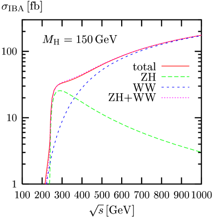
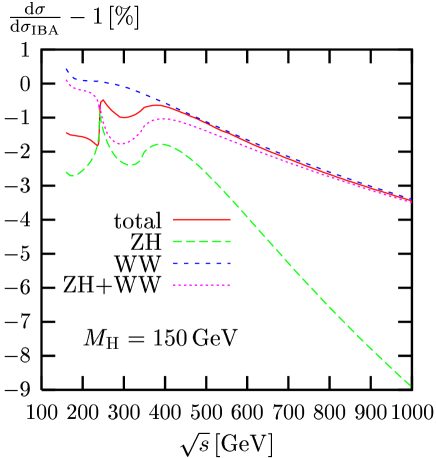
Figure 11: Improved Born approximation (IBA) for the total cross sections and radiative corrections relative to the IBA for $M_{\mathrm{H}}=150\,\mathrm{GeV}$

Analogous results have been given in Ref. [21] for the pure lowest-order cross sections $\sigma_{\mathrm{tree}}$ and the corresponding relative corrections (see Figs. 1 and 2 there). While the absolute cross sections $\sigma_{\mathrm{IBA}}$ and $\sigma_{\mathrm{tree}}$ look qualitatively similar, the relative corrections normalized to the $\sigma_{\mathrm{IBA}}$ are systematically smaller as compared to a normalization to the pure lowest-order cross section. This is mainly due to the dominance of the ISR corrections which are properly taken into account by the IBA. In the WW channel the IBA describes the corrected cross section within 1% for CM energies up to $\sim 500\,\mathrm{GeV}$ and remains still good within 2–3% up to $\sqrt{s}\mathrel{\raisebox{-3.00003pt}{$\stackrel{{\scriptstyle\displaystyle<}}{{\sim}}$}}1\,\mathrm{TeV}$. At high CM energies the IBA misses non-universal bosonic corrections, the size of which grows with energy (compare Fig. 3 of Ref. [21]). In the ZH channel the IBA deviates from the corrected cross section by $\mathrel{\raisebox{-3.00003pt}{$\stackrel{{\scriptstyle\displaystyle<}}{{\sim}}$}}3\%$ for $\sqrt{s}\mathrel{\raisebox{-3.00003pt}{$\stackrel{{\scriptstyle\displaystyle<}}{{\sim}}$}}500\,\mathrm{GeV}$, but even this reasonably good approximation results from accidental compensations between fermionic and bosonic non-ISR corrections, which are both of the order of 5–10% but of opposite sign (see Fig. 3 of Ref. [21]). Above a CM energy of $500\,\mathrm{GeV}$, where ZH production is suppressed, the IBA becomes even worse, since the dominating Sudakov logarithms, such as $\alpha\ln^{2}(s/M_{\mathrm{W}}^{2})$ are missing in the IBA.

In Figure 12 the cross sections and their corrections are shown as functions of the Higgs-boson mass $M_{\mathrm{H}}$ for the typical LC energy of $\sqrt{s}=500\,\mathrm{GeV}$.

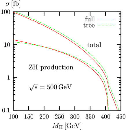
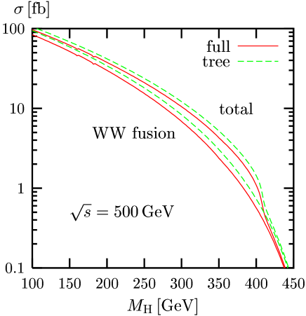
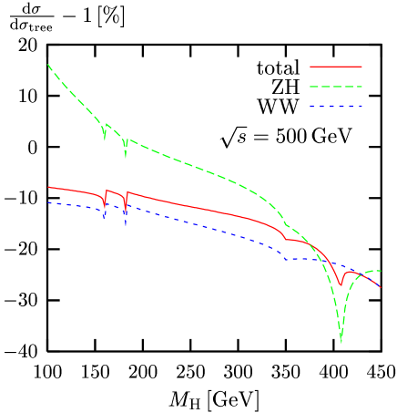
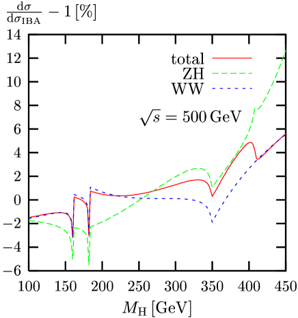
Figure 12: Cross sections and relative corrections as function of the Higgs-boson mass for $\sqrt{s}=500\,\mathrm{GeV}$

For this CM energy the contribution of WW fusion is much larger than the one of ZH production for $M_{\mathrm{H}}\mathrel{\raisebox{-3.00003pt}{$\stackrel{{\scriptstyle\displaystyle<}}{{\sim}}$}}300\,\mathrm{GeV}$. For $M_{\mathrm{H}}\mathrel{\raisebox{-3.00003pt}{$\stackrel{{\scriptstyle\displaystyle>}}{{\sim}}$}}\sqrt{s}-M_{\mathrm{Z}}\approx 409\,\mathrm{GeV}$ the ZH-production channel is strongly suppressed since the Z boson cannot become resonant there. The total cross section falls below $1\,\mathrm{fb}$ in this domain. For $M_{\mathrm{H}}\mathrel{\raisebox{-3.00003pt}{$\stackrel{{\scriptstyle\displaystyle<}}{{\sim}}$}}350\,\mathrm{GeV}$ the relative corrections to the total cross section and to the WW-fusion channel are of the order $-10\%$ to $-20\%$ if normalized to $\sigma_{\mathrm{tree}}$, but only at the level of 2% if normalized to $\sigma_{\mathrm{IBA}}$. For the ZH-production channel the reduction of the relative corrections with respect to $\sigma_{\mathrm{IBA}}$ is similar. The spikes at $M_{\mathrm{H}}=2M_{\mathrm{W}},2M_{\mathrm{Z}},2m_{\mathrm{t}}$ result from thresholds. These singularities are avoided if the finite widths of the unstable particles are taken into account appropriately (see, for instance, Ref. [51]).

3.3 Results on distributions

The distributions in the Higgs-boson energy $E_{\mathrm{H}}$ (defined in the CM frame) are depicted in Figure 13 for $\sqrt{s}=500\,\mathrm{GeV}$ and $M_{\mathrm{H}}=150\,\mathrm{GeV}$.

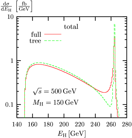
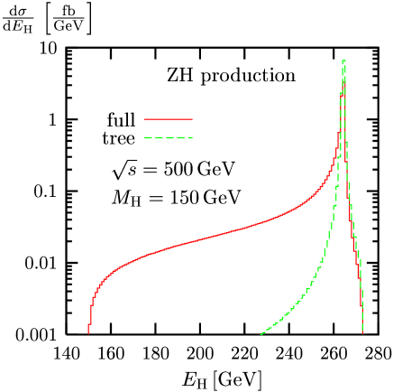
Figure 13: Distribution in the Higgs-boson energy $E_{\mathrm{H}}$ and corresponding relative radiative corrections for $\sqrt{s}=500\,\mathrm{GeV}$ and $M_{\mathrm{H}}=150\,\mathrm{GeV}$

The broad continuous distribution for $E_{\mathrm{H}}\mathrel{\raisebox{-3.00003pt}{$\stackrel{{\scriptstyle\displaystyle<}}{{\sim}}$}}250\,\mathrm{GeV}$ is almost entirely due to WW fusion, while the resonance peak at $E_{\mathrm{H}}\sim 265\,\mathrm{GeV}$ corresponds to the Higgs-boson energy in the $2\to 2$ kinematics of the ZH-production process with an on-shell Z boson. This explains the behaviour of the radiative corrections, which are dominated by ISR. Since the WW-fusion cross section rises with energy, the continuous part receives negative corrections. For the WW-fusion channel these are particularly large for large $E_{\mathrm{H}}$ near the phase space boundary. On the other hand, the Z peak is reduced by ISR and produces a radiative tail for $E_{\mathrm{H}}$ values below the peak, since ISR effectively reduces the scattering energy of the subsequent ZH-production process. This radiative tail leads to corrections of up to 220%, as can be seen in the inset of the lower left plot in Figure 13. The relative corrections are reduced drastically if normalized to the IBA, which takes care of the large ISR effects. For $E_{\mathrm{H}}\mathrel{\raisebox{-3.00003pt}{$\stackrel{{\scriptstyle\displaystyle<}}{{\sim}}$}}250\,\mathrm{GeV}$ the corrections to the total improved-Born cross section vary only weakly with $E_{\mathrm{H}}$.

Figure 14 illustrates the distribution in the cosine of the Higgs-boson production angle $\theta_{\mathrm{H}}$ (defined in the CM frame) for $\sqrt{s}=500\,\mathrm{GeV}$ and $M_{\mathrm{H}}=150\,\mathrm{GeV}$.

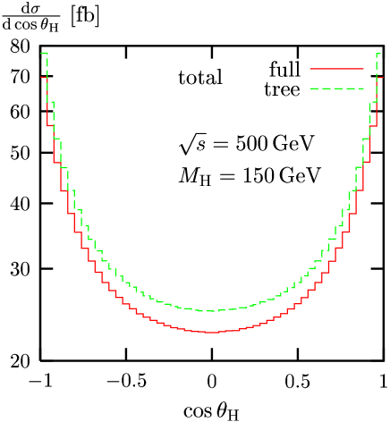
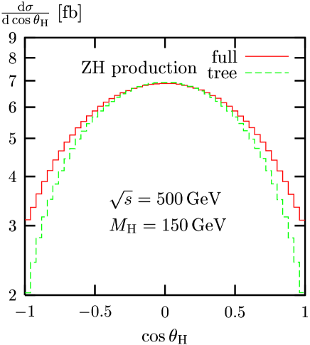
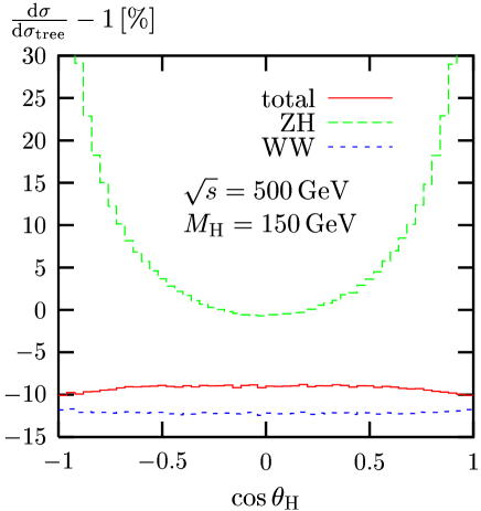
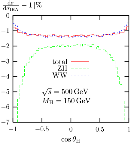
Figure 14: Distribution in the cosine of the Higgs-boson production angle $\theta_{\mathrm{H}}$ and corresponding relative radiative corrections for $\sqrt{s}=500\,\mathrm{GeV}$ and $M_{\mathrm{H}}=150\,\mathrm{GeV}$

The peak behaviour in the very forward and backward directions is due to the dominant WW contribution, while ZH production follows a shape roughly proportional to $1-\cos^{2}\theta_{\mathrm{H}}$. The relative corrections to the WW contribution depend only weakly on $\cos\theta_{\mathrm{H}}$ and reflect the same reduction after normalization to the IBA as the integrated cross sections. The relative corrections to the ZH contribution become large in the forward and backward directions, where the corresponding lowest-order cross section is small.

Finally, we show the spectra of the photon energy $E_{\gamma}$ and the photon polar angle $\cos\theta_{\gamma}$ (both defined in the CM frame) of the radiative process ${\mathrm{e^{+}}}{\mathrm{e^{-}}}\to\nu\bar{\nu}{\mathrm{H}}+\gamma$ for $\sqrt{s}=500\,\mathrm{GeV}$ and $M_{\mathrm{H}}=150\,\mathrm{GeV}$.

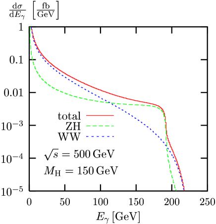
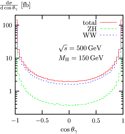
Figure 15: Distribution in the photon energy $E_{\gamma}$ and in the photon polar angle $\cos\theta_{\gamma}$ in the radiative process ${\mathrm{e^{+}}}{\mathrm{e^{-}}}\to\nu\bar{\nu}{\mathrm{H}}+\gamma$ for $\sqrt{s}=500\,\mathrm{GeV}$ and $M_{\mathrm{H}}=150\,\mathrm{GeV}$

In order to make the photon visible, we impose angular and energy cuts of

$$\theta(\gamma,\mathrm{beam})>1^{\circ}\qquad E_{\gamma}>0.1\,\mathrm{GeV}.$$ (3.3)

For small photon energies the infrared pole, which is the same for the WW and ZH channels, dominates the spectrum. Thus, WW fusion dominates for small $E_{\gamma}$, since the lowest-order cross section is much larger for WW fusion than for ZH production. For larger $E_{\gamma}$, small-angle photon emission is dominant as some kind of remnant of the collinear pole for forward and backward emission. This means that larger $E_{\gamma}$ reflect the lowest-order cross sections at smaller energies. Since the ZH-production cross section rises with decreasing CM energies for $\sqrt{s}\mathrel{\raisebox{-3.00003pt}{$\stackrel{{\scriptstyle\displaystyle<}}{{\sim}}$}}500\,\mathrm{GeV}$, but the WW-fusion cross section falls off steeply, ZH production takes over the leading role for $E_{\gamma}\mathrel{\raisebox{-3.00003pt}{$\stackrel{{\scriptstyle\displaystyle>}}{{\sim}}$}}110\,\mathrm{GeV}$.

3.4 Comparison to related work

Adapting the input parameters and the parametrization of the lowest-order matrix element to those used by Belanger et al. [18], we reproduced the numbers for the total cross section given in Table 2 of the first paper of Ref. [18]. Note that we switch off the ISR beyond ${\cal{O}}(\alpha)$ in this comparison. In Table 1 we list for each Higgs-boson mass and the corresponding calculated W-boson mass the results of Ref. [18] together with our results. The numbers in parenthesis indicate the errors in the last digits.

$$\begin{array}[]{c@{\qquad}c@{\qquad}l@{\qquad}l@{\qquad}l@{\ \ }l}\hline\cr M_{\mathrm{H}}~{}[\mathrm{GeV}]&M_{\mathrm{W}}~{}[\mathrm{GeV}]&\;\sigma_{{\mathrm{tree}}}~{}[\mathrm{fb}]&\ \sigma~{}[\mathrm{fb}]{}&\sigma/\sigma_{{\mathrm{tree}}}-1~{}[\%]\\ \hline\cr 150&80.3767&61.074(7)&60.99(7)&-0.2&\mathrm{\mbox{Ref.~{}\cite[cite]{[\@@bibref{}{Belanger:2002me}{}{}]}}}\\ &&61.076(5)&60.80(2)&-0.44(3)&\mathrm{this~{}work}\\ \hline\cr 200&80.3571&37.294(4)&37.16(4)&-0.4&\mathrm{\mbox{Ref.~{}\cite[cite]{[\@@bibref{}{Belanger:2002me}{}{}]}}}\\ &&37.293(3)&37.09(2)&-0.56(4)&\mathrm{this~{}work}\\ \hline\cr 250&80.3411&21.135(2)&20.63(2)&-2.5&\mathrm{\mbox{Ref.~{}\cite[cite]{[\@@bibref{}{Belanger:2002me}{}{}]}}}\\ &&21.134(1)&20.60(1)&-2.53(3)&\mathrm{this~{}work}\\ \hline\cr 300&80.3275&10.758(1)&10.30(1)&-4.2&\mathrm{\mbox{Ref.~{}\cite[cite]{[\@@bibref{}{Belanger:2002me}{}{}]}}}\\ &&10.7552(7)&10.282(4)&-4.40(3)&\mathrm{this~{}work}\\ \hline\cr 350&80.3158&4.6079(5)&4.184(4)&-9.1&\mathrm{\mbox{Ref.~{}\cite[cite]{[\@@bibref{}{Belanger:2002me}{}{}]}}}\\ &&4.6077(2)&4.181(1)&-9.27(3)&\mathrm{this~{}work}\\ \hline\cr\end{array}$$

Table 1: Total cross section in lowest order and including the full ${\cal{O}}(\alpha)$ corrections and the relative corrections for $\sqrt{s}=500\,\mathrm{GeV}$ and various Higgs masses for the input parameter scheme of Ref. [18]¹

The agreement is good; the relative differences are with one exception below $10^{-4}$ for the total lowest-order cross section and below 0.3% for the corrected cross section. The corrections relative to the lowest-order cross section agree within 0.2%. This is of the order of the statistical error of Ref. [18], which is about 0.1%. Note that Belanger et al. use $\alpha(0)$ to parametrize the lowest-order cross section. As a consequence their relative corrections are shifted by $3\Delta r\approx+9\%$ compared to those in the $G_{\mu}$-scheme.

We have also reproduced the $\cos\theta_{\mathrm{H}}$ and $E_{\mathrm{H}}$ distributions in Figures 1 and 2 of the first paper of Ref. [18]. We found agreement within the accuracy of these figures.

When considering only fermion-loop corrections, we find agreement with the calculations of Refs. [19, 20], once the appropriate renormalization and input-parameter schemes are adopted. For more details on this comparison we refer to Ref. [21].

4 Summary

We have presented a calculation of the complete electroweak ${\cal O}(\alpha)$ radiative corrections to the single Higgs-boson production process ${\mathrm{e^{+}}}{\mathrm{e^{-}}}\to\nu\bar{\nu}{\mathrm{H}}$ in the electroweak Standard Model. For ${\mathrm{e^{+}}}{\mathrm{e^{-}}}\to\nu_{\mathrm{e}}\bar{\nu}_{\mathrm{e}}{\mathrm{H}}$, where ${\mathrm{Z}}{\mathrm{H}}$ production and W-boson fusion contribute, both production channels are added coherently. Two methods for the treatment of the finite Z-boson width have been introduced. We have taken special care to treat the contributions from 5-point tensor integrals in a numerically stable way. The complete single-hard-photon matrix elements have been taken into account, where soft and collinear singularities are treated both in the subtraction and the phase-space slicing methods. Higher-order ISR corrections have been included in the structure-function approach. The phase-space integration is performed with Monte-Carlo techniques.

We find that the electroweak corrections are of the order of $-10\%$ and are dominated by ISR corrections if the lowest-order matrix element is parametrized with the Fermi constant $G_{\mu}$. The non-ISR corrections are at the level of a few per cent in the $G_{\mu}$-scheme, but are of the order of 10% in other schemes. At high energies, where the WW-fusion channel dominates, the electroweak corrections depend only weakly on the energy and the production angle of the Higgs-boson.

Although the sum of ISR and non-ISR is accidentally small in the $\alpha(0)$-scheme, the $G_{\mu}$-scheme is nevertheless preferable for the following reasons. In contrast to the $\alpha(0)$ scheme, it does not suffer from uncertainties arising from the hadronic vacuum polarization at low energies. Since the cancellation between ISR and non-ISR corrections in the $\alpha(0)$ scheme at one loop is accidental, it cannot be expected that it still holds in higher orders. One the other hand, the $G_{\mu}$-scheme resums the leading universal corrections associated with the running of the electromagnetic coupling and the universal corrections proportional to the square of the top mass.

We have shown that the corrections to the WW-fusion channel can be described by a simple improved Born approximation within an accuracy of typically 1% (3%) for CM energies below $500\,\mathrm{GeV}$ ($1\,\mathrm{TeV}$). For the ZH-production channel the improved Born approximation, which is simply based on ISR, approximates the corrected cross section within 3% up to CM energies of about $500\,\mathrm{GeV}$, but becomes worse at higher energies. In summary, the approximation can be used to include radiative corrections at the qualitative level, but a precision analysis will require the inclusion of the full ${\cal O}(\alpha)$ correction.

Appendix

Standard matrix elements

The four-dimensionality of space–time implies that the SME $\hat{\cal{M}}^{{\mathrm{ZH}},\sigma}_{i}$ and $\hat{\cal{M}}^{{\mathrm{WW}}}_{i}$ introduced in Section 2.1 are not all independent; there are linear relations among them.

A simple way to derive the relations with real coefficients is provided by the following trick. In four dimensions the metric tensor can be decomposed in terms of four independent orthonormal four-vectors $n_{l}$,

$$g^{\alpha\beta}=n_{0}^{\alpha}n_{0}^{\beta}-\sum_{l=1}^{3}n_{l}^{\alpha}n_{l}^{\beta},$$ (A.1)

where $n_{k}\cdot n_{l}=g_{kl}$. Two convenient choices ($j=1,2$) for the vectors $n_{l}$ are given by

$$n_{0}^{\alpha} = \frac{1}{\sqrt{s}}(p_{1}+p_{2})^{\alpha},\qquad n_{1}^{\alpha}=\frac{1}{\sqrt{s}}(p_{1}-p_{2})^{\alpha},$$

$$n_{2}^{\alpha} = \sqrt{\frac{s}{t_{1j}t_{2j}}}\left(k_{j}^{\alpha}+\frac{t_{2j}}{s}p_{1}^{\alpha}+\frac{t_{1j}}{s}p_{2}^{\alpha}\right),\quad$$

$$n_{3}^{\alpha} = \epsilon^{\alpha\beta\gamma\delta}n_{0,\beta}n_{1,\gamma}n_{2,\delta}=-\frac{2}{\sqrt{st_{1j}t_{2j}}}\epsilon^{\alpha\beta\gamma\delta}p_{1,\beta}p_{2,\gamma}k_{j,\delta},$$ (A.2)

with $\epsilon^{\alpha\beta\gamma\delta}$ ($\epsilon^{0123}=+1$) denoting the totally antisymmetric tensor. Inserting this decomposition for both $j=1,2$ in all contractions between different Dirac chains according to $\Gamma^{{\mathrm{e}}{\mathrm{e}},\sigma}_{\alpha}\Gamma^{\nu\nu,\alpha}=\Gamma^{{\mathrm{e}}{\mathrm{e}},\sigma}_{\alpha}g^{\alpha\beta}\Gamma^{\nu\nu}_{\beta}$, etc., and subsequently using the Dirac equation and the Chisholm identity

$${\mathrm{i}}\epsilon^{\alpha\beta\gamma\delta}\gamma_{\delta}\gamma_{5}=\gamma^{\alpha}\gamma^{\beta}\gamma^{\gamma}-g^{\alpha\beta}\gamma^{\gamma}+g^{\alpha\gamma}\gamma^{\beta}-g^{\beta\gamma}\gamma^{\alpha},$$ (A.3)

reduces all ZH SME $\hat{\cal{M}}^{{\mathrm{ZH}},\sigma}_{i}$ to four and all WW SME $\hat{\cal{M}}^{{\mathrm{WW}}}_{i}$ to two SME.

Further relations with complex coefficients result from the direct application of the Chisholm identity (A.3) to structures like $\Gamma^{\nu\nu}_{k_{1}p_{1}k_{2}}$ and subsequently using the decomposition

$$g^{\rho\sigma}=\sum_{i,j=1}^{4}\left(Z^{-1}\right)_{ij}2p_{i}^{\rho}p_{j}^{\sigma},\qquad Z_{ij}=2p_{i}p_{j},\qquad p_{3}=k_{1},\quad p_{4}=k_{2},$$ (A.4)

to separate all contractions between $\epsilon$ tensors and Dirac chains via $\Gamma^{\nu\nu}_{\delta}\epsilon^{\alpha\beta\gamma\delta}=\Gamma^{\nu\nu}_{\rho}g^{\rho\sigma}\epsilon^{\alpha\beta\gamma}_{\phantom{\alpha\beta\gamma}\sigma}$. For $\Gamma^{\nu\nu}_{k_{1}p_{1}k_{2}}$, in particular, this leads to

$$\Gamma^{\nu\nu}_{\delta}\epsilon^{k_{1}p_{1}k_{2}\delta}=\Gamma^{\nu\nu}_{\rho}g^{\rho\sigma}\epsilon^{k_{1}p_{1}k_{2}}_{\phantom{k_{1}p_{1}k_{2}}\sigma}=-2X\left[\Gamma^{\nu\nu}_{p_{1}}\left(Z^{-1}\right)_{12}+\Gamma^{\nu\nu}_{p_{2}}\left(Z^{-1}\right)_{22}\right]$$ (A.5)

with

$$X=\epsilon^{p_{1}p_{2}k_{1}k_{2}}=\epsilon^{\mu\nu\rho\sigma}p_{1,\mu}p_{2,\nu}k_{1,\rho}k_{2,\sigma}.$$ (A.6)

In the inverse matrix $\left(Z^{-1}\right)$, the determinant $\det(Z)$ occurs, which can be identified with $\det(Z)=-16X^{2}$.

Altogether, the linear relations reduce the set of ZH SME to two and the set of WW SME to one SME. Explicitly, the relations read

$$\hat{\cal{M}}^{{\mathrm{ZH}},\pm}_{i}=r_{i}^{{\mathrm{ZH}},\pm}\hat{\cal{M}}^{{\mathrm{ZH}},+}_{1},\qquad\hat{\cal{M}}^{{\mathrm{WW}}}_{i}=r_{i}^{{\mathrm{WW}}}\hat{\cal{M}}^{{\mathrm{WW}}}_{1},\qquad i=2,\ldots 13,$$ (A.7)

with

$$\begin{array}[b]{lllllllll}r^{{\mathrm{ZH}},+}_{2}&=&s,&r^{{\mathrm{ZH}},-}_{2}&=&0,&r^{{\mathrm{WW}}}_{2}&=&-t_{11},\\ r^{{\mathrm{ZH}},+}_{3}&=&0,&r^{{\mathrm{ZH}},-}_{3}&=&s_{12},&r^{{\mathrm{WW}}}_{3}&=&0,\\ r^{{\mathrm{ZH}},+}_{4}&=&0,&r^{{\mathrm{ZH}},-}_{4}&=&\frac{1}{2}C^{*},&r^{{\mathrm{WW}}}_{4}&=&\frac{1}{2}C,\\ r^{{\mathrm{ZH}},+}_{5}&=&\frac{1}{4t_{22}}A,&r^{{\mathrm{ZH}},-}_{5}&=&-\frac{t_{11}}{2},&r^{{\mathrm{WW}}}_{5}&=&\frac{s}{2},\\ r^{{\mathrm{ZH}},+}_{6}&=&-\frac{t_{21}}{2},&r^{{\mathrm{ZH}},-}_{6}&=&\frac{1}{4t_{12}}A^{*},&r^{{\mathrm{WW}}}_{6}&=&-\frac{1}{4t_{12}}B^{*},\\ r^{{\mathrm{ZH}},+}_{7}&=&-\frac{t_{12}}{2},&r^{{\mathrm{ZH}},-}_{7}&=&\frac{1}{4t_{21}}A,&r^{{\mathrm{WW}}}_{7}&=&-\frac{1}{4t_{21}}B,\\ r^{{\mathrm{ZH}},+}_{8}&=&\frac{1}{4t_{11}}A^{*},&r^{{\mathrm{ZH}},-}_{8}&=&-\frac{t_{22}}{2},&r^{{\mathrm{WW}}}_{8}&=&\frac{s_{12}}{2},\\ r^{{\mathrm{ZH}},+}_{9}&=&\frac{1}{t_{22}}A,&r^{{\mathrm{ZH}},-}_{9}&=&-4t_{11},&r^{{\mathrm{WW}}}_{9}&=&4s,\\ r^{{\mathrm{ZH}},+}_{10}&=&-2t_{21},&r^{{\mathrm{ZH}},-}_{10}&=&\frac{2}{t_{12}}A^{*},&r^{{\mathrm{WW}}}_{10}&=&-\frac{2}{t_{12}}B^{*},\\ r^{{\mathrm{ZH}},+}_{11}&=&-2t_{12},&r^{{\mathrm{ZH}},-}_{11}&=&-4t_{12},&r^{{\mathrm{WW}}}_{11}&=&-4t_{12},\\ r^{{\mathrm{ZH}},+}_{12}&=&\frac{1}{t_{11}}A^{*}&r^{{\mathrm{ZH}},-}_{12}&=&-4t_{22},&r^{{\mathrm{WW}}}_{12}&=&4s_{12},\\ r^{{\mathrm{ZH}},+}_{13}&=&4,&r^{{\mathrm{ZH}},-}_{13}&=&16,&r^{{\mathrm{WW}}}_{13}&=&16\end{array}$$ (A.8)

and

$$A = ss_{12}-t_{12}t_{21}-t_{11}t_{22}+4{\mathrm{i}}X,$$

$$B = ss_{12}+t_{12}t_{21}-t_{11}t_{22}+4{\mathrm{i}}X,$$

$$C = ss_{12}-t_{12}t_{21}+t_{11}t_{22}+4{\mathrm{i}}X.$$ (A.9)

Finally, there are Fierz identities relating the ZH and WW spinor chains, supplementing the above list of relations by

$$\hat{\cal{M}}^{{\mathrm{WW}}}_{1}=-\hat{\cal{M}}^{{\mathrm{ZH}},-}_{1},$$ (A.10)

so that all SME can be expressed in terms of $\hat{\cal{M}}^{{\mathrm{ZH}},\pm}_{1}$. In terms of Weyl–van der Waerden spinor products, which have been defined in Section 2.3.1 (see also Ref. [38]), these SME read

$$\hat{\cal{M}}^{{\mathrm{ZH}},+}_{1}=2\langle p_{2}k_{2}\rangle^{*}\langle p_{1}k_{1}\rangle,\qquad\hat{\cal{M}}^{{\mathrm{ZH}},-}_{1}=2\langle p_{1}k_{2}\rangle^{*}\langle p_{2}k_{1}\rangle.$$ (A.11)

Since the lowest-order matrix elements for right- and left-handed electrons are proportional to $\hat{\cal{M}}^{{\mathrm{ZH}},+}_{1}$ and $\hat{\cal{M}}^{{\mathrm{ZH}},-}_{1}$, respectively, the whole virtual one-loop contributions to the squared matrix element are of the form

$$\mathop{\mathrm{Re}}\nolimits\left\{{\cal{M}}_{1}^{\sigma}\left({\cal{M}}_{0}^{\sigma}\right)^{*}\right\}=\left[f_{1}^{\sigma}(s,t_{ij},s_{ij})+f_{2}^{\sigma}(s,t_{ij},s_{ij})X\right]|\hat{\cal{M}}_{1}^{{\mathrm{ZH}},\sigma}|^{2},$$ (A.12)

where $f^{\sigma}_{i}$ are functions of scalar products of the external momenta. Note that the $f^{\sigma}_{i}$ and $|\hat{\cal{M}}_{1}^{{\mathrm{ZH}},\sigma}|^{2}$ are invariant under the reflection of all outgoing momenta ${\bf k}_{j}$ on the plane spanned by the beam axis and the Higgs-boson momentum ${\bf k}_{3}$, while $X$ changes its sign under this reflection. Consequently, the contribution proportional to $X$ drops out after integrating over the momenta of the final-state neutrinos, which are not observable.

References

- [1] ATLAS collaboration, ATLAS Detector and Physics Performance Technical Design Report, CERN-LHWW 99-14.
- [2] CMS collaboration, CMS Technical Proposal, CERN-LHWW 94-38.
- [3] The LEP Working Group for Higgs Boson Searches, LHWG Note/2002-01.
- [4] E. Accomando et al. [ECFA/DESY LC Physics Working Group Collaboration], Phys. Rept. 299 (1998) 1 [hep-ph/9705442].
- [5] J. A. Aguilar-Saavedra et al., TESLA Technical Design Report Part III: Physics at an Linear Collider [hep-ph/0106315].
- [6] K. Abe et al. [ACFA Linear Collider Working Group Collaboration], ACFA Linear Collider Working Group report, [hep-ph/0109166].
- [7] T. Abe et al. [American Linear Collider Working Group Collaboration], in Proc. of the APS/DPF/DPB Summer Study on the Future of Particle Physics (Snowmass 2001) ed. R. Davidson and C. Quigg, SLAC-R-570, Resource book for Snowmass 2001 [hep-ex/0106055, hep-ex/0106056, hep-ex/0106057, hep-ex/0106058].
-
[8]
E. Accomando, A. Ballestrero and M. Pizzio,
in Linear Colliders: Physics and Detector Studies Part
E, ed. R. Settles (DESY 97-123E, Hamburg, 1997), p. 31
[hep-ph/9709277] and
Nucl. Phys. B 547 (1999) 81
[hep-ph/9807515];
G. Montagna, M. Moretti, O. Nicrosini and F. Piccinini, Eur. Phys. J. C 2 (1998) 483 [hep-ph/9705333];
F. Gangemi, G. Montagna, M. Moretti, O. Nicrosini and F. Piccinini, Eur. Phys. J. C 9 (1999) 31 [hep-ph/9811437]. - [9] S. Dittmaier and M. Roth, Nucl. Phys. B 642 (2002) 307 [hep-ph/0206070].
-
[10]
J. R. Ellis, M. K. Gaillard and D. V. Nanopoulos,
Nucl. Phys. B 106 (1976) 292;
B. L. Ioffe and V. A. Khoze, Sov. J. Part. Nucl. 9 (1978) 50 [Fiz. Elem. Chast. Atom. Yadra 9 (1978) 118]. - [11] J. D. Bjorken, in Weak Interactions at High-Energy and the Production of New Particles: Proceedings of the 4th Slac Summer Institute on Particle Physics, ed. M. C. Zipf (SLAC-198, Stanford, 1976) p. 1.
- [12] J. Fleischer and F. Jegerlehner, Nucl. Phys. B 216 (1983) 469.
- [13] B. A. Kniehl, Z. Phys. C 55 (1992) 605.
- [14] A. Denner, J. Küblbeck, R. Mertig and M. Böhm, Z. Phys. C 56 (1992) 261.
- [15] F. A. Berends and R. Kleiss, Nucl. Phys. B 260 (1985) 32.
-
[16]
D. R. Jones and S. T. Petcov,
Phys. Lett. B 84 (1979) 440;
G. Altarelli, B. Mele and F. Pitolli, Nucl. Phys. B 287 (1987) 205;
W. Kilian, M. Krämer and P. M. Zerwas, Phys. Lett. B 373 (1996) 135 [hep-ph/9512355];
E. Boos, M. Sachwitz, H. J. Schreiber and S. Shichanin, Int. J. Mod. Phys. A 10 (1995) 2067. - [17] F. Jegerlehner and O. Tarasov, hep-ph/0212004.
- [18] G. Belanger, F. Boudjema, J. Fujimoto, T. Ishikawa, T. Kaneko, K. Kato and Y. Shimizu, hep-ph/0211268; hep-ph/0212261.
- [19] H. Eberl, W. Majerotto and V. C. Spanos, Phys. Lett. B 538 (2002) 353 [hep-ph/0204280]; hep-ph/0210038; hep-ph/0210330.
- [20] T. Hahn, S. Heinemeyer and G. Weiglein, hep-ph/0211204; hep-ph/0211384.
- [21] A. Denner, S. Dittmaier, M. Roth and M. M. Weber, hep-ph/0301189.
- [22] W. F. L. Hollik, Fortsch. Phys. 38 (1990) 165.
-
[23]
J. Küblbeck, M. Böhm and A. Denner,
Comput. Phys. Commun. 60 (1990) 165;
H. Eck and J. Küblbeck, Guide to FeynArts 1.0, University of Würzburg, 1992. - [24] G. Passarino and M. Veltman, Nucl. Phys. B 160 (1979) 151.
- [25] G. ’t Hooft and M. Veltman, Nucl. Phys. B 153 (1979) 365.
- [26] W. Beenakker and A. Denner, Nucl. Phys. B 338 (1990) 349.
- [27] A. Denner, Fortsch. Phys. 41 (1993) 307.
- [28] A. Denner and S. Dittmaier, hep-ph/0212259.
- [29] W. Beenakker, S. Dittmaier, M. Krämer, B. Plümper, M. Spira and P. M. Zerwas, hep-ph/0211352, to appear in Nucl. Phys. B.
- [30] A. Denner, S. Dittmaier and G. Weiglein, Nucl. Phys. B 440 (1995) 95 [hep-ph/9410338].
- [31] T. Hahn, Comput. Phys. Commun. 140 (2001) 418 [hep-ph/0012260].
-
[32]
T. Hahn and M. Perez-Victoria,
Comput. Phys. Commun. 118 (1999) 153
[hep-ph/9807565];
T. Hahn, Nucl. Phys. Proc. Suppl. 89 (2000) 231 [hep-ph/0005029]. - [33] R. Mertig, M. Böhm and A. Denner, Comput. Phys. Commun. 64 (1991) 345.
-
[34]
D. Y. Bardin, A. Leike, T. Riemann and M. Sachwitz,
Phys. Lett. B 206 (1988) 539;
D. Wackeroth and W. Hollik, Phys. Rev. D 55 (1997) 6788 [hep-ph/9606398];
W. Beenakker et al., Nucl. Phys. B 500 (1997) 255 [hep-ph/9612260]. - [35] S. Dittmaier and M. Krämer, Phys. Rev. D 65 (2002) 073007 [hep-ph/0109062].
- [36] G. Burgers and F. Jegerlehner, in Physics at LEP 1, eds. G. Altarelli, R. Kleiss and C. Verzegnassi (CERN 99-08, Geneva, 1989), p. 7.
- [37] B. A. Kniehl and M. Steinhauser, Nucl. Phys. B 454 (1995) 485 [hep-ph/9508241].
- [38] S. Dittmaier, Phys. Rev. D 59 (1999) 016007 [hep-ph/9805445].
-
[39]
T. Stelzer and W. F. Long,
Comput. Phys. Commun. 81 (1994) 357
[hep-ph/9401258];
H. Murayama, I. Watanabe and K. Hagiwara, KEK-91-11. - [40] S. Catani and M. H. Seymour, Phys. Lett. B 378 (1996) 287 [hep-ph/9602277] and Nucl. Phys. B 485 (1997) 291 [Erratum-ibid. B 510 (1997) 291] [hep-ph/9605323].
- [41] S. Dittmaier, Nucl. Phys. B 565 (2000) 69 [hep-ph/9904440].
- [42] M. Roth, PhD thesis, ETH Zürich No. 13363 (1999), hep-ph/0008033.
- [43] M. Böhm and S. Dittmaier, Nucl. Phys. B409 (1993) 3 and B412 (1994) 39.
- [44] D.R. Yennie, S.C. Frautschi and H. Suura, Ann. Phys. 13 (1961) 379.
-
[45]
E.A. Kuraev and V.S. Fadin,
Yad. Fiz. 41 (1985) 753 [Sov. J. Nucl. Phys. 41 (1985) 466];
G. Altarelli and G. Martinelli, in Physics at LEP, eds. J. Ellis and R. Peccei, (CERN 86-02, Geneva, 1986), Vol. 1, p. 47;
O. Nicrosini and L. Trentadue, Phys. Lett. B196 (1987) 551; Z. Phys. C39 (1988) 479;
F.A. Berends, G. Burgers and W.L. van Neerven, Nucl. Phys. B297 (1988) 429, E:B304 (1988) 921. - [46] W. Beenakker et al., in Physics at LEP2, eds. G. Altarelli, T. Sjöstrand and F. Zwirner (CERN 96-01, Geneva, 1996), Vol. 1, p. 79 [hep-ph/9602351].
- [47] A. Denner, S. Dittmaier, M. Roth and D. Wackeroth, Nucl. Phys. B 560 (1999) 33 [hep-ph/9904472].
- [48] G. P. Lepage, J. Comput. Phys. 27 (1978) 192 and CLNS-80/447.
- [49] K. Hagiwara et al. [Particle Data Group Collaboration], Phys. Rev. D 66 (2002) 010001.
- [50] F. Jegerlehner, DESY 01-029, LC-TH-2001-035, hep-ph/0105283.
-
[51]
T. Bhattacharya and S. Willenbrock,
Phys. Rev. D 47 (1993) 4022;
B. A. Kniehl, C. P. Palisoc and A. Sirlin, Nucl. Phys. B 591 (2000) 296 [hep-ph/0007002].