Choice of heavy baryon currents in QCD sum rules

Abstract

In this paper we investigate the effects due to the mixing of two interpolating currents for ground state baryons within the framework of Heavy Quark Effective Theory using the QCD sum rule approach. Both two-point and three-point sum rules, thus the mass, coupling constant and Isgur-Wise function sum rules are considered. It is interesting to contrast those results with each other. Based on the Isgur-Wise functions obtained in this paper, we also analyze the effects of current mixing to $\Lambda$- type and and $\Sigma$-type semi-leptonic decays $\Lambda_{b}\rightarrow\Lambda_{c}l\bar{\nu}$, $\Sigma_{b}\rightarrow\Sigma_{c}\ell\bar{\nu}$ and $\Sigma_{b}\rightarrow\Sigma^{*}_{c}\ell\bar{\nu}$. Decay widths corresponding to various mixing parameters are obtained and can be compared to the experimental data.

I Introduction

Strong interactions between quarks can be well described by QCD in the standard model. Recently important progresses in the theoretical description of hadrons containing a heavy quark have been achieved with the development of the Heavy Quark Effective Theory (HQET) HQET ; review ; KKP . Based on the spin-flavor symmetry of QCD, exactly valid in the infinite heavy quark mass limit, $m_{Q}\rightarrow\infty$, this framework provides a systematic expansion of heavy hadron spectra and both the strong and weak transition amplitudes in terms of the leading contribution, plus corrections decreasing as powers of $1/m_{Q}$. HQET has been applied successfully to learn about the properties of meson and baryon made of both heavy and light quarks.

Due to the asymptotic freedom of QCD, non-perturbative effect plays an important role in the hadronic physics. Thus it is inevitable to employ some non-perturbative technique in strong interaction related problems. QCD sum rule svzsum formulated in the framework of HQET hqetsum is a desirable approach and proves to be predictive Braun99 . This method allows one to relate hadronic observable to QCD parameter via the operator product expansion (OPE) of the correlator. The choice of the interpolating current for a state with given spin and parity is the first step in the application of QCD sum rule method. Principally, if a current is chosen within the framework of HQET, QCD sum rule can be applied to many fields without ambiguity and successfully. But the real situation is not so simple. The main problem lies just on the choice of the interpolating currents. On the heavy meson side, the current interpolating a given spin and parity ground state is unique for it constitutes of one heavy and one light quark. However, on the heavy baryon side, the interpolating current is not uniqueDHLL ; GrYa ; Ivanov . For a given state there exist two commonly adopted interpolating currents. Both bear the general form as GrYa ; Ioff

$$j^{\,v}=\epsilon_{abc}(q^{T\,a}_{1}\,C\Gamma\,\tau\,q^{b}_{2})\Gamma^{\prime}h_{v}^{c},$$ (1)

in which $C$ is the charge conjugation matrix, $\tau$ is the flavor matrix which is antisymmetric for $\Lambda_{Q}$ baryon and symmetric for $\Sigma_{Q}^{(*)}$ baryon, $\Gamma$ and $\Gamma^{\prime}$ are some gamma matrices, and a, b, c denote the color indices. One kind of current’s $\Gamma$ and $\Gamma^{\prime}$ can be chosen covariantly as

$$\Gamma=\gamma_{5}\;,\hskip 28.45274pt\Gamma^{\prime}=1\;,$$ (2)

for $\Lambda_{Q}$ baryon,

$${}\Gamma=\gamma_{\mu}\;,\hskip 28.45274pt\Gamma^{\prime}=(\gamma_{\mu}+v_{\mu})\,\gamma_{5}\;,$$ (3)

for $\Sigma_{Q}$ baryon, and

$$\Gamma=\gamma_{\nu}\;,\hskip 14.22636pt\Gamma^{\prime}=-g_{\mu\nu}+\frac{1}{3}\gamma_{\mu}\,\gamma_{\nu}-\frac{1}{3}(\gamma_{\mu}\,v_{\nu}-\gamma_{\nu}\,v_{\mu})+\frac{2}{3}v_{\nu}\,v_{\mu}\;,$$ (4)

for $\Sigma_{Q}^{*}$ baryon. Another kind of current can be obtained by inserting a factor $\hbox to0.0pt{/\hss}v$ behind the $\Gamma$ matrices defined by equations (2)-(4). We denote them as $j^{v}_{1}$ and $j^{v}_{\,2}$, respectively. In QCD sum rule applications those two currents are usually used separatelyDHLL ; GrYa ; WHL ; DHHL ; HLLS ; GKY ; CDNP . Constituent quark type current which is the linear combination of the two previously defined currents with the same coefficient can also be found in applicationGKY2 . But generally speaking, the interpolating current should be the linear combination of the two currents with arbitrary coefficients. And also there have been many papers treating just the question of the choice of baryon currents both in full QCD and in HQET sum rulesChung ; Bagan . In this paper we adopt the general form $j^{v}=a\,j^{v}_{\,1}+b\,j^{v}_{\,2}$, in which the coefficients $a$ and $b$ can be arbitrary real numbers, to investigate the effects of different choice of baryon currents on physical observable.

The baryon coupling constants in HQET are defined through the vacuum-to-baryon matrix element of the interpolating current as follows

$$\langle 0\mid j^{v}\mid\Lambda(v)\rangle = F_{\Lambda}\,u\,,$$

$$\langle 0\mid j^{v}\mid\Sigma(v)\rangle = F_{\Sigma}\,u\,,$$

$$\langle 0\mid j^{v}\mid\Sigma^{*}(v)\rangle = \frac{1}{\sqrt{3}}\,F_{\Sigma^{*}}\,u^{\alpha}\;,$$ (5)

where $u$ is the spinor and $u_{\alpha}$ is the Rarita-Schwinger spinor in the HQET, respectively. The coupling constants $F_{\Sigma}$ and $F_{\Sigma}^{*}$ are equivalent since $\Sigma_{Q}$ and $\Sigma_{Q}^{*}$ belong to the doublet with the same spin-parity of the light degrees of freedom.

The remainder of this paper is organized as follows. In Sec. II we focus our emphasis on two-point and three-point correlators and thus obtained sum rules for ground state baryons. In Sec. II.1 mass sum rules and in Sec. II.2 sum rules for Isgur-Wise functions are presented. Sec. III is devoted to numerical results and our conclusions.

II Two-point and three-point correlators

II.1 Two-point correlator and mass sum rule

Two-point correlators are T-product of interpolating currents saturated between vacuum

$$i\int dx\,e^{ik\cdot x}\langle 0\mid T\{j^{v}(x)\bar{j}^{v}(0)\}\mid 0\rangle=\Gamma^{\prime}\frac{1+\hbox to0.0pt{/\hss}v}{2}\bar{\Gamma}^{\prime}Tr[\tau\tau^{+}]\Pi(\omega),$$ (6)

where $k$ is the residual momentum and $\omega=2v\cdot k$. The QCD sum rule determination of baryon coupling constants can be achieved by analyzing the two-point correlator. These diagonal correlators of the single interpolating currents have been obtained long ago by many authors and are of the same form for both the interpolating currents $j_{1}^{v}$ and $j_{2}^{v}$. Non-diagonal correlators have been analyzed in Ref.GrYa in the leading order in $\alpha_{s}$ and in next to leading order in $\alpha_{s}$ in Ref.GKY . In our previous worksWHL ; DHHL ; HLLS we adopted the diagonal correlator as the starting point since for the non-diagonal correlator there is no perturbative contribution under the usual assumption of quark-hadron duality, let alone to be the dominant part to the sum rules derived. Here we only have one unique interpolating current and there is only one diagonal correlator and no non-diagonal case to be analyzed. Our theoretical result thus is the combination of the previously called diagonal and non-diagonal results. It should be noted that the non-diagonal one is merely treated as power corrections of OPE in our choice of current.

In our calculations condensates with a dimension higher than $6$ are not included for lack of information and radiative corrections are out of consideration contemporarily. In order to obtain an estimate of the dimension $3$ nonlocal quark condensate we adopt the gaussian ansatz $\langle\bar{q}(0)q(x)\,\rangle=\langle\bar{q}q\rangle\mbox{exp}(m_{0}^{2}x^{2}/16)$. Relevant Feynman diagrams are presented in Fig. 1. Then it is straightforward to obtain the two-point sum rules:

$$2\,F^{2}_{\Lambda}\;e^{-2\bar{\Lambda}_{\Lambda}/T} = (a^{2}+b^{2})\left[\frac{3\,T^{6}}{2^{4}\,\pi^{4}}\,\delta_{5}(\omega_{c}/T)+\frac{T^{2}}{2^{6}\,\pi^{2}}\,\langle\frac{\alpha_{s}}{\pi}G^{2}\rangle\ +\frac{1}{3}\,\langle\bar{q}q\rangle^{2}\,e^{-m_{0}^{2}/2T^{2}}\right]$$

$$- \frac{a\,b}{\pi^{2}}\langle\bar{q}q\rangle[T^{3}\,e^{-m_{0}^{2}/4T^{2}}+T\,\frac{m_{0}^{2}}{8}],$$

$$\frac{2}{3}F^{2}_{\Sigma}\;e^{-2\bar{\Lambda}_{\Sigma}/T} = (a^{2}+b^{2})\left[\frac{3\,T^{6}}{2^{4}\;\pi^{4}}\,\delta_{5}(\omega_{c}/T)-\frac{T^{2}}{3\,2^{6}\,\pi^{2}}\,\langle\frac{\alpha_{s}}{\pi}G^{2}\rangle+\frac{1}{3}\,\langle\bar{q}q\rangle^{2}\,e^{-m_{0}^{2}/2T^{2}}\right]$$ (7)

$$- \frac{a\,b}{\pi^{2}}\langle\bar{q}q\rangle[T^{3}\,e^{-m_{0}^{2}/4T^{2}}-T\,\frac{m_{0}^{2}}{24}].$$

Our two-point sum rules do agree with results previously obtained in Refs.GrYa ; WHL . The functions $\delta_{n}(\omega_{c}/T)$ arise from the continuum subtraction and are given by

$$\delta_{n}(x)=\frac{1}{n!}\int\limits_{0}^{x}\!\mbox{d}t\,t^{n}e^{-t}=1-e^{-x}\sum_{k=0}^{n}\frac{x^{k}}{k!}\,.$$ (8)

The second term of the last equation is assigned to the continuum mode, which can be much larger than the ground state contribution for the typical value of parameter T if the dimension of the spectral densities are very high.

II.2 Three-point sum rules

For a heavy-heavy velocity changing current ${\cal J}=\bar{h}\Gamma\bar{h}^{\prime}$ we can define a three-point correlator in which $J$ is inserted between two interpolating currents as below

$$i^{2}\int dx_{1}dx_{2}\;e^{i(k\cdot x_{1}-k^{\prime}\cdot x_{2})}\langle 0\mid T\{j^{\,v}(x_{1}){\cal J}(0)\bar{j}^{\,v^{\prime}}(x_{2})\}\mid 0\rangle =$$

$$\Gamma^{\prime}\frac{1+\hbox to0.0pt{/\hss}v}{2}\Gamma\frac{1+\hbox to0.0pt{/\hss}v^{\prime}}{2}\bar{\Gamma}^{\prime}Tr[\tau\tau^{+}]\;T(\omega,\omega^{\prime},y)\;,$$ (9)

where $T(\omega,\omega^{\prime},y)$ is analytic function in the “off-shell energies” $\omega=2v\cdot k$ and $\omega^{\prime}=2v^{\prime}\cdot k^{\prime}$ with discontinuities for positive values of these variables. It furthermore depends on the velocity transfer $y=v\cdot v^{\prime}$, which is fixed at its physical region for the process under consideration. In the heavy quark limit, the matrix element of current ${\cal J}$ can be parameterized by one or two scalar functions of $y$. Those scalar functions are called Isgur-Wise functionsIW and can be defined as

$$\langle\Lambda_{Q}|\bar{h}\Gamma h^{\prime}|\Lambda_{Q^{\prime}}\rangle=\xi(y)\,\bar{u}\,\Gamma\,u^{\prime},$$ (10)

for $\Lambda$-type baryon, and

$$\langle\Sigma_{Q}|\bar{h}\Gamma h^{\prime}|\Sigma_{Q^{\prime}}\rangle=[-\xi_{1}(y)g_{\mu\nu}+\xi_{2}(y)v^{\prime}_{\mu}v_{\nu}]\,\bar{\Psi}_{\mu}\Gamma\,\Psi^{\prime}_{\nu},$$ (11)

for $\Sigma$-type baryon, in which $u$ is the Dirac spinor as defined in (I) and $\Psi_{\mu}$ is the covariant representation of the spin $1/2$ doublets $\Psi_{\mu}=u_{\mu}+\frac{1}{\sqrt{3}}(v_{\mu}+\gamma_{\mu})u$. Both $\xi(y)$ and $\xi_{1}(y)$ are normalized to unity at the zero recoil $y=1$ due to the heavy quark symmetry. However, one cannot invoke symmetry arguments to predict the normalization at $y=1$ of $\xi_{2}(y)$.

Saturating the three-point correlator with complete set of baryon states, one can divide it into two parts. One is the part of interest, the contribution of the lowest-lying baryon states associated with the heavy-heavy currents, as one having poles in both the variables $\omega$ and $\omega^{\prime}$ at the value $\omega=\omega^{\prime}=2\bar{\Lambda}$. The other contribution to the correlator comes from higher resonant states. For the little knowledge of this part of contribution it is common to resort to the quark-hadron duality, which insures that continuum contribution can be approximated by the integral of the perturbative spectral density over a continuum threshold, to get a predictive result.

On theoretical side the scalar function $T(\omega,\omega^{\prime},y)$ can be calculated using quark and gluon language with vacuum condensates. Dispersion relation enables one to express the correlator in the form of integrals of the double spectral density as

$$T(\omega,\omega^{\prime},y)=\int_{0}^{\infty}\int_{0}^{\infty}\frac{\mbox{d}s}{s-\omega}\frac{\mbox{d}s^{\prime}}{s^{\prime}-\omega^{\prime}}\,\rho(\mbox{s},\mbox{s}^{\prime},y).$$ (12)

With the redefinition of the integral variablesDHLL ; HLLS ; IWfun ; Neubert92D

$$s_{+} = \frac{s+s^{\prime}}{2},$$

$$s_{-} = \left(\frac{y-1}{y+1}\right)^{1/2}\frac{s-s^{\prime}}{2},$$ (13)

the integration domain becomes

$$\int_{0}^{\infty}ds\int_{0}^{\infty}ds^{\prime}=2\left(\frac{y-1}{y+1}\right)^{1/2}\int_{0}^{\infty}ds_{+}\int_{-s_{+}}^{s_{+}}ds_{-}.$$ (14)

It is in variable $s_{+}$ that the commonly adopted quark-hadron duality is assumedNeubert92D ; BS

$$res.=2\left(\frac{y-1}{y+1}\right)^{1/2}\int_{\omega^{\prime}_{c}}^{\infty}ds_{+}\int_{-s_{+}}^{s_{+}}ds_{-}\frac{\rho(\mbox{s},\mbox{s}^{\prime},y)}{(s-\omega)(s^{\prime}-\omega^{\prime})},$$ (15)

and for simplicity we take $\omega^{\prime}_{c}$ to be equal to the two-point continuum threshold $\omega_{c}$: $\omega^{\prime}_{c}=\omega_{c}$.

In our theoretical calculations of the three-point correlator only condensates with dimension no more than 6 are included. Order $1/m_{Q}$ power corrections and radiative corrections are not included in present calculations, either. For their contributions to the correlator only amount to several percents and do not change the numerical result dramatically. Also the gaussian ansatz for the nonlocal quark condensate is adopted. Feynman diagrams related to the calculations of three-point correlator are shown in Fig. 2.

Then following the standard procedure we resort to the Borel transformation $B^{\omega}_{\tau}$, $B^{\omega^{\prime}}_{\tau^{\prime}}$ to suppress the contributions of the excited states. Considered the symmetry of the correlation function it is natural to set the parameters $\tau$, $\tau^{\prime}$ to be the same and equal to 2T, where T is the Borel parameter of the two-point sum rules. Finally, we obtain the sum rules for the Isgur-Wise functions as

$$4F_{\Lambda}^{2}\,\xi(y)\,e^{-2\bar{\Lambda}_{\Lambda}/T} = \frac{3\,(a^{2}+b^{2})}{\pi^{4}\,(1+y)^{3}}T^{6}\delta_{5}(\omega_{c}/T)+\frac{[a^{2}(2y+1)+b^{2}y(y+2)]\,T^{2}}{24(1+y)^{2}\pi^{2}}\langle\frac{\alpha_{s}}{\pi}G^{2}\rangle$$

$$+ \frac{2\,(a^{2}+b^{2}y)}{3}\langle\bar{q}q\rangle^{2}e^{-(1+y)m_{0}^{2}/4T^{2}}-\frac{4a\,b\langle\bar{q}q\rangle}{(1+y)\pi^{2}}[T^{3}\,e^{-m_{0}^{2}(1+y)/8T^{2}}+T\,\frac{m_{0}^{2}}{24}(y+2)],$$

$$\frac{4}{3}F_{\Sigma}^{2}\,\xi_{1}(y)\,e^{-2\bar{\Lambda}_{\Sigma}/T} = \frac{3\,(a^{2}+b^{2})}{\pi^{4}\,(1+y)^{3}}T^{6}\delta_{5}(\omega_{c}/T)-\frac{(a^{2}+b^{2})\,T^{2}}{24(1+y)^{2}\pi^{2}}\langle\frac{\alpha_{s}}{\pi}G^{2}\rangle$$

$$+ \frac{2\,(a^{2}+b^{2}y)}{3}\langle\bar{q}q\rangle^{2}e^{-(1+y)m_{0}^{2}/4T^{2}}-\frac{4a\,b\langle\bar{q}q\rangle}{(1+y)\pi^{2}}[T^{3}\,e^{-m_{0}^{2}(1+y)/8T^{2}}-T\,\frac{m_{0}^{2}}{24}y],$$

$$\frac{4}{3}F_{\Sigma}^{2}\,\xi_{2}(y)\,e^{-2\bar{\Lambda}_{\Sigma}/T} = \frac{3\,(a^{2}+b^{2}y)}{\pi^{4}\,(1+y)^{4}}T^{6}\delta_{5}(\omega_{c}/T)+\frac{(a^{2}y-b^{2})\,T^{2}}{24(1+y)^{3}\pi^{2}}\langle\frac{\alpha_{s}}{\pi}G^{2}\rangle$$ (16)

$$+ \frac{2\,b^{2}}{3}\langle\bar{q}q\rangle^{2}e^{-(1+y)m_{0}^{2}/4T^{2}}-\frac{4a\,b\langle\bar{q}q\rangle}{(1+y)^{2}\pi^{2}}[T^{3}\,e^{-m_{0}^{2}(1+y)/8T^{2}}+T\,\frac{m_{0}^{2}}{24}(y-2)],$$

The unitary normalization of flavor matrix $Tr[\tau\tau^{+}]=1$ has been applied to get those sum rules. It is obvious that the normalization of the Isgur-Wise functions $\xi(y)$ and $\xi_{1}(y)$ at zero recoil is satisfied automatically.

III numerical results and conclusions

It is obvious that in the expressions of two-point and three-point sum rules the relative value of the two parameters but not the absolute value plays an important role. So in this section we change the current mixing parameters $a,b$ to one angular variable $\theta$ through relations $b/a=\tan\theta$ where $\theta$ can be restrained to the range $\theta\in[-\pi/2,\pi/2]$, in which $\theta=0,\pm\pi/2$ correspond to the diagonal cases. In the numerical analysis we will investigate the current mixing effects in those sum rules. Standard values of the vacuum condensates are

$$\langle\bar{q}q\rangle=-(0.23\;\mbox{GeV})^{3},$$

$$\langle\frac{\alpha_{s}}{\pi}G^{2}\rangle=0.012\;\mbox{GeV}^{4},$$

$$\langle\bar{q}g\sigma_{\mu\nu}G^{\mu\nu}q\rangle=m_{0}^{2}\langle\bar{q}q\rangle,\;\;\;m_{0}^{2}=0.8\;\mbox{GeV}^{2}.$$ (17)

They will be used in the following numerical analysis of the sum rules.

III.1 mass sum rules

In the analysis of the coupling constant sum rules we need the effective mass of the baryons in consideration as the input parameter. One way to obtain this parameter is to extract it from the experimental data assuming the heavy quark mass to be the commonly recognized value from the outset of the analysis. For the aim of consistency we adopt another way of obtaining the effective mass parameter from Eq. (II.1) which is based on the QCD sum rule method entirely. The effective mass can be expressed through the derivative of Borel variable T in the coupling constant sum rules as

$$\bar{\Lambda}=-\frac{1}{2}\frac{\partial}{\partial T^{-1}}\ln\,\mbox{K(T)},$$ (18)

in which K(T) denotes the right hand side of Eq.(II.1). So the first step of our numerical analysis of those two-point sum rules is to find the value of the effective mass. But the second step, which is the analysis of coupling constant sum rules, will be omitted here as the focus of our interest is on the mass sum rules entirely. Our main idea in the consideration of the effect of the current mixing parameter to the sum rules is to see if there exists a reasonable stability window of the Borel parameter T under the variation of $\theta$ in the range from $-\pi/2$ to $\pi/2$. For the analysis of the coupling constant and mass sum rules it is enough to take $\theta$ from $0$ to $\pi/2$ for on the range of $\theta$ from $-\pi/2$ to $0$ the mass sum rules oscillate for the Borel parameter $\mbox{T}\sim 1\;\mbox{GeV}$ so sharply that it is impossible to find a desirable stability window. Thus we do not take into account of that half part of $\theta$.

For the $\Lambda$-type baryon mass sum rule we find that there is no agreeable stability window except around the vicinity of $\theta=0$ or $\theta=\pi/2$, i.e. $a=1,b=0$ or $a=0,b=1$. So there is no or at most little space left for the mixing of currents and what we obtained is the diagonal sum rule. It is reasonable to assume this result does indicate that there exists some mechanism which forbids the mixing of the two sector interpolating currents in the mass sum rule in the leading order. The diagonal sum rule result can be checked with previous work: When $\omega_{c}$ lies between $1.9\sim 2.5\;\mbox{GeV}$ there exists the stability window $0.35<\mbox{T}<0.65\;\mbox{GeV}$. The effective mass thus obtained is $\bar{\Lambda}_{\Lambda}=0.73\pm 0.07\;\mbox{GeV}$, in which the error only reflects the variation of Borel parameter T and continuum threshold $\omega_{c}$.

For the $\Sigma$-type baryon all sum rule windows are narrower than that of $\Lambda$-type baryon and the stability is not as good as that of $\Lambda$-type baryon, eitherGrYa . With the increasing of $\theta$ the stability falls drastically that the optional space left for the variation of $\theta$ is smaller than that of $\Lambda$-type baryon. When $\omega_{c}$ lies between $2.8\sim 3.3\;\mbox{GeV}$ there exists the stability window $0.4<\mbox{T}<0.7\;\mbox{GeV}$ for the diagonal sum rules, which appear to be the only surviving result with respect to the mixing of currents. The effective mass thus obtained is $\bar{\Lambda}_{\Sigma}=0.90\pm 0.14\;\mbox{GeV}$, in which the error only reflects the variation of Borel parameter T and continuum threshold $\omega_{c}$, too. Those results can be checked with Refs.GrYa ; WHL . It is also worth noting that the constituent quark type interpolating current cannot be distinguished from the currents with arbitrary mixing parameters from the stability point of view. Both $\Lambda$-type and $\Sigma$-type mass sum rules are presented in Fig. 3.

III.2 sum rules for the three-point correlators

III.2.1 Isgur-Wise functions

In order to get the numerical results for the Isgur-Wise functions, we divide our three-point sum rules by two-point functions to obtain $\xi$, $\xi_{1}$ and $\xi_{2}$ as functions of the continuum threshold $\omega_{c}$ and the Borel parameter T. This procedure can eliminate the systematic uncertainties and cancel the dependence on mass parameter $\bar{\Lambda}$. As for the mixing parameter $\theta$ in this part, we take it varying from $-\pi/2$ to $\pi/2$ to determine the stability of the sum rules.

For the Isgur-Wise function of the $\Lambda$-type baryon, $\xi(y)$, we find that it is not sensitive to the mixing parameter $\theta$. Almost in the gamut of $\theta$ there exists a stability window, and the stability does not change rapidly when $\theta$ goes far beyond the vicinity of the diagonal $\theta$s. The continuum threshold is the same as that for the two-point sum rule for the $\Lambda$-type baryon. For $\omega_{c}$ lies between $1.9\sim 2.5\;\mbox{GeV}$ there exists the stability window. The stability window for $\xi(y=1.2)$ is a much narrower one, $0.4<\mbox{T}<0.8\;\mbox{GeV}$. The numerical results are shown in Fig. 4. In the numerical analysis it is interesting that there seems to exist a more stable window for the constituent quark type current with $\theta=\pi/4$, though the tendency is not so predominant.

The numerical analysis of the two Isgur-Wise functions of the $\Sigma$-type baryon can be compared with each other. For the function $\xi_{1}$, the existence of stability window can only allow for the appearance of two diagonal sum rules and one constituent quark type sum rule with mixing parameter $\theta=-\pi/4$. As for the function $\xi_{2}$, the existence of stability window can allow for the appearance of two diagonal sum rules besides one constituent quark type sum rule with mixing parameter $\theta=\pi/4$. When the continuum threshold $\omega_{c}$ lies between $2.5\sim 3.3\;\mbox{GeV}$ there exist the stability windows for both functions with the allowed mixing angles. The numerical results of two Isgur-Wise functions are shown in Fig. 5. Due to lack of stability window of those two constituent quark type sum rules with the mixing parameters $\theta=\pm\pi/4$ for $\xi_{1}$ and $\xi_{2}$, both numerical results related to those two sum rules are taken from the range $0.8<\mbox{T}<1.2$, the continuum threshold is the same as that of the diagonal sum rules. We also present our results for the function $\xi_{2}(1)$ in Table  1. Our results of the two constituent quark type currents are approximately equal to 0.5 at the zero recoil, which is consistent with the value obtained from constituent quark model and large $N_{c}$ limit in Refs.korner ; Chow .

$\theta$  ($\tan\theta=b/a$)	$\theta=0$	$\theta=\pi/4$	$\theta=\pi/2$	$\theta=-\pi/4$	Refs.korner ; Chow
$\xi_{2}(1)$	$0.40\pm 0.07$	$0.51\pm 0.01$	$0.62\pm 0.07$	$0.48\pm 0.01$	$0.5$

Table 1: The value of Isgur-Wise function $\xi_{2}$ at the zero recoil.

If we put the two Isgur-Wise functions which are normalized to unity at the zero recoil into the linear form $\xi_{(1)}(y)=1-\rho_{(1)}^{2}(y-1)$, in which the parameters $\rho^{2}$ and $\rho_{1}^{2}$ are the slopes (or charge radii) of the Isgur-Wise functions, we can obtain the slopes $\rho^{2}$ and $\rho_{1}^{2}$ via a linear fit for $\xi(y)$ and $\xi_{1}(y)$ near the zero recoil. The final results of the slopes are presented in Table  2. Many predictions have been made on the value of the charge radii, and the results vary greatly from each otherIvanov ; DHHL ; JMW ; prd56-348 ; MNNFD ; IL .

radii	$\theta=0$	$\theta=\pi/4$	$\theta=\pi/2$	$\theta=-\pi/4$
$\rho^{2}$	$0.66\pm 0.08$	$0.46\pm 0.03$	$0.35\pm 0.13$	$0.41\pm 0.10$
$\rho_{1}^{2}$	$0.80\pm 0.07$	$0.58\pm 0.08$	$0.57\pm 0.18$	$0.30\pm 0.11$

Table 2: Charge radii $\rho^{2}$ and $\rho_{1}^{2}$ for the Isgur-Wise functions $\xi(y)$ and $\xi_{1}(y)$.

III.2.2 semi-leptonic decay rates

With the appropriate forms for the Isgur-Wise functions $\xi,\,\xi_{1}\,\mbox{and}\,\xi_{2}$ as we have derived in Eq. (II.2), we can discuss various semi-leptonic decays involving the heavy-to-heavy transition $b\rightarrow c$. As some illustrative examples here we shall only consider three types of semi-leptonic decays: $\Lambda_{b}\rightarrow\Lambda_{c}\,\ell\bar{\nu}$, $\Sigma_{b}\rightarrow\Sigma_{c}\,\ell\bar{\nu}$ and $\Sigma_{b}\rightarrow\Sigma^{*}_{c}\,\ell\bar{\nu}$.

The semi-leptonic decay $\Lambda_{b}\rightarrow\Lambda_{c}\ell\bar{\nu}$ can be analyzed directly after obtaining the Isgur-Wise function from the QCD sum rules. By neglecting the lepton mass, the differential decay rate is DHHL

$$\frac{1}{\sqrt{y^{2}-1}}\frac{d\Gamma(\Lambda_{b}\rightarrow\Lambda_{c}l\bar{\nu})}{dy}=\frac{G_{F}^{2}|V_{cb}|^{2}m_{\Lambda_{b}}^{2}m_{\Lambda_{c}}^{3}}{(2\pi)^{3}}$$

$$\times\{(1-2ry+r^{2})[(y-1)F_{1}^{2}+(y+1)G_{1}^{2}]+\frac{y^{2}-1}{3}(Ar^{2}+2Br+C)\},$$ (19)

where $r=m_{\Lambda_{c}}/m_{\Lambda_{b}}$. In the above equation,

$$A = 2F_{1}F_{2}+(y+1)F_{2}^{2}+2G_{1}G_{2}+(y-1)G_{2}^{2},$$

$$B = F_{1}^{2}+F_{1}F_{2}+F_{2}F_{3}+F_{3}F_{1}+yF_{2}F_{3}+G_{1}^{2}-G_{1}G_{2}-G_{2}G_{3}+G_{3}G_{1}+yG_{2}G_{3},$$

$$C = (y+1)F_{3}^{2}+2F_{1}F_{3}+(y-1)G_{3}^{2}-2G_{1}G_{3}.$$ (20)

To the next to leading order of $1/m_{Q}$, the form factors $F_{i}$ and $G_{i}$ bear the simple form

$$F_{1} = C(\mu)\xi(y)+\left(\frac{\bar{\Lambda}}{2m_{c}}+\frac{\bar{\Lambda}}{2m_{b}}\right)[2\chi(y)+\xi(y)],$$

$$G_{1} = C(\mu)\xi(y)+\left(\frac{\bar{\Lambda}}{2m_{c}}+\frac{\bar{\Lambda}}{2m_{b}}\right)[2\chi(y)+\frac{y-1}{y+1}\xi(y)],$$

$$F_{2} = G_{2}=-\frac{\bar{\Lambda}}{m_{c}(y+1)}\xi(y),$$

$$F_{3} = -G_{3}=-\frac{\bar{\Lambda}}{m_{b}(y+1)}\xi(y),$$ (21)

where $C(\mu)$ is the perturbative QCD coefficient, $\chi(y)$ is the sub-leading order Isgur-Wise function, which is only amounts to the order of a few percents to the leading function and can be safely neglectedDHHL ; KorMel . With the form of the leading order Isgur-Wise function (12), the differential decay rate of $\Lambda_{b}\rightarrow\Lambda_{c}l\bar{\nu}$ is shown in Fig. 5. In this analysis, we choose those related heavy quark masses to be: $m_{b}=4.77\;\mbox{GeV},m_{c}=1.41\;\mbox{GeV}$WHL , and parameters $m_{\Lambda_{b}}=5.641\;\mbox{GeV},m_{\Lambda_{c}}=2.285\;\mbox{GeV}$ can be found in Ref.data , the renormalization point is $\mu=470\;\mbox{MeV}$. It seems to be inconsistent to use the quark masses obtained in Ref.WHL using factorization instead of gaussian ansatz to parameterize the non-local quark condensate as done in Ref.DHLL . But the fact that the decay width is not sensitive to the heavy quark masses allows us to use either pair of parameters without varying the width significantly. The decay widths corresponding to four typical mixing variables are listed in Table 3. Also listed in Table 3 are some predictions made by QCD sum rule and other phenomenological approaches. The averages of the decay widths are taken between $0.8<\mbox{T}<1.1\;\mbox{GeV}$ and $1.9\leq\omega_{c}\leq 2.5\;\mbox{GeV}$. Our results are in good consistence with the experimental value, $\Gamma=(4.0\pm 1.0)\times 10^{-14}\mbox{GeV}$data .

As to the two decays between $\Sigma$-type baryons, the decay widths have simple and easy-to-be-interpreted forms when expressed with helicity amplitudes. Related formulae can be found in many referencesKKP ; prd56-348 ; EIKL and the decay widths corresponding to various mixing parameters are listed in Table 3. In this part of numerical analysis we only take into account of the contributions of the leading order Isgur-Wise functions and omit the higher order effects. The masses of the heavy baryons are taken to be $m_{\Sigma_{b}}=5.80\;\mbox{GeV}$WHL , $m_{\Sigma^{*}_{c}}=2.52\;\mbox{GeV}$ and $m_{\Sigma_{c}}=2.455\;\mbox{GeV}$data . For comparison we list the results for those three types of decays predicted by QCD sum rule and other phenomenological approaches in Table 3, too. It should be noted here that function $\xi_{1}$ is the predominant part in the decay rates, so even though for the mixing parameter $\theta=-\pi/4$ there exists no stability window for function $\xi_{2}$, the total decay rates still have a mild stability window for $\theta=-\pi/4$.

Refs.		$\Lambda_{b}\rightarrow\Lambda_{c}\ell\bar{\nu}$	$\Sigma_{b}\rightarrow\Sigma_{c}\ell\bar{\nu}$	$\Sigma_{b}\rightarrow\Sigma^{*}_{c}\ell\bar{\nu}$
	$\theta=0$	$4.57\pm 0.62$	$1.38\pm 0.15$	$2.89\pm 0.16$
	$\theta=\pi/4$	$3.98\pm 0.07$	$1.66\pm 0.11$	$2.78\pm 0.06$
this paper	$\theta=\pi/2$	$3.60\pm 0.29$	$1.50\pm 0.25$	$2.94\pm 0.22$
	$\theta=-\pi/4$	$3.97\pm 0.13$	$2.09\pm 0.24$	$3.27\pm 0.38$
RTQM  Ivanov		$4.08$	$1.51$	$2.48$
RTQM prd56-348		$3.521$	$1.468$	$3.001$
RTQM  IL		$3.769$	$0.946$	$2.171$
QCMEIKL		$6.582$	$3.226$
SQM  single		$3.883$	$2.830$

Table 3: Decay widths $\Gamma(\mbox{in}\,10^{-14}\,\mbox{GeV})$ for the semi-leptonic decays $\Lambda_{b}\rightarrow\Lambda_{c}l\bar{\nu}$, $\Sigma_{b}\rightarrow\Sigma_{c}l\bar{\nu}$ and $\Sigma_{b}\rightarrow\Sigma^{*}_{c}l\bar{\nu}$. Also presented in this table are some phenomenological predictions using Relativistic Three-Quark Model(RTQM), Quark Confinement Model(QCM) and Spectator Quark Model(SQM).

For conclusions, we have investigated the mixing of currents interpolating ground heavy baryon state within the framework of HQET using QCD sum rule approach. For the two-point sum rules there can only survive the diagonal ones and the constituent quark type current is not preferable from the stability point of view for both $\Lambda$-type and $\Sigma$-type baryons. As for the three-point sum rules, Isgur-Wise function $\xi(y)$ for $\Lambda$-type baryon is not sensitive to the mixing parameter and the stability window exists almost for all the range of mixing parameter; on the other hand, Isgur-Wise function $\xi_{1}(y)$ and $\xi_{2}(y)$ allows for two diagonal, one constituent($\theta=\pi/4$) and one anti-constituent($\theta=-\pi/4$) quark type sum rules. The effect of different currents to semi-leptonic decays $\Lambda_{b}\rightarrow\Lambda_{c}l\bar{\nu}$, $\Sigma_{b}\rightarrow\Sigma_{c}\ell\bar{\nu}$ and $\Sigma_{b}\rightarrow\Sigma^{*}_{c}\ell\bar{\nu}$ has also been analyzed in this paper. We find that the current mixing effects in those processes are not significant.

Figure Captions

Fig. 1. Non-vanishing diagrams for the two-point correlator: (a) perturbative contribution, (b) quark-condensate, (c) gluon-condensate, (d) mixed condensate, (e) four-quark condensate contributions. The interpolating baryonic currents are denoted by black circles. Heavy-quark propagators are drawn as double curves.

Fig. 2. Non-vanishing diagrams for the three-point correlator: (a) perturbative contribution, (b) quark-condensate, (c) and (d) gluon-condensate, (e) mixed condensate and (f) four-quark condensate. The velocity-changing current operator is denoted by a white square, and the interpolating baryonic currents by black circles.

Fig. 3. Sum rules for effective mass parameter $\bar{\Lambda}$: The left one is for $\Lambda$-type baryon, in which $\omega_{c}=2.2\;\mbox{GeV}$; and the right one is for $\Sigma$-type baryon, in which $\omega_{c}=2.8\;\mbox{GeV}$.

Fig. 4. Sum rules of the Isgur-Wise function $\xi(y)$ with various mixing parameters. The threshold in this figure is $\omega_{c}=2.2\;\mbox{GeV}$ and the momentum transfer is $y=1.1$.

Fig. 5. Sum rules of Isgur-Wise function $\xi_{1}(y)$ and $\xi_{2}(y)$ with various mixing parameters. The threshold in this figure is $\omega_{c}=2.8\;\mbox{GeV}$ and the momentum transfer is $y=1.1$.

Fig. 6. Differential decay ratio of semi-leptonic decay $\Lambda_{b}\rightarrow\Lambda_{c}l\bar{\nu}$ with various mixing parameters as below: (a) $\theta=0$, (b) $\theta=\pi/4$, (c) $\theta=\pi/2$ and (d) $\theta=-\pi/4$. The solid, dashed and dotted curves correspond to the threshold $\omega_{c}=1.9,2.2,2.5\;\mbox{GeV}$, respectively. And the Borel parameter is $\mbox{T}=0.85\,\mbox{GeV}$ in this figure.

Figure 1:

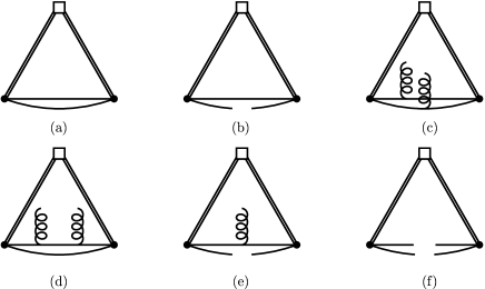
Figure 2:

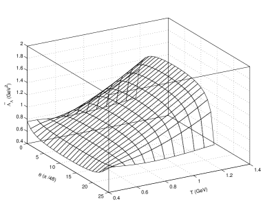
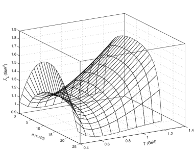
Figure 3:

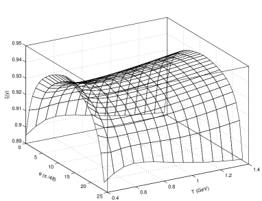
Figure 4:

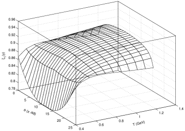
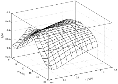
Figure 5:

Figure 6: