hep-ph/0302189
New Ideas in Symmetry Breaking 

Abstract

Some old and new ideas on symmetry breaking, based on the presence of extra dimensions that have been the subject of a very fast development and intensive studies during the last years, will be presented in these lectures. Special attention will be devoted to the various compactification mechanisms, including toroidal and orbifold compactifications, and to non-trivial boundary conditions or Scherk-Schwarz compactification. Also symmetry breaking by Wilson lines, or Hosotani breaking characteristic of non-simply connected compact manifolds will be analyzed in some detail. The different mechanisms will be applied to the breaking of the most relevant symmetries in particle physics: supersymmetry and gauge symmetry. The required background for these lectures is Quantum Field Theory, Supersymmetry and some rudiments of Kaluza-Klein theory. The different sections will be illustrated with examples.

1 Introduction

Symmetry breaking is one of the main issues in contemporary particle physics. Its implementation in a perturbative quantum field theory has led to the notion of spontaneous symmetry breaking with the presence of a massless Goldstone particle for the case of a global symmetry (Goldstone theorem [1]) and a massive Higgs particle for a local symmetry (Higgs mechanism [2]). These ideas based on four dimensional field theories are nowadays thoroughly explained in many textbooks in quantum field theory [3].

The idea of unification of all interactions led to the introduction of extra dimensions starting from the pioneer work of Kaluza and Klein who attempted to unify gravity and electromagnetism through the presence of a fifth dimension [4]. More recently the attempts to unify gravity with electroweak and strong interactions in a consistent quantum theory have led to the modern string theories that incorporate supersymmetries and are described in ten (heterotic, type II and type I strings) or eleven (M-theory) space-time dimensions [5]. The recent string dualities relating all string constructions [6] as well as the presence in the spectrum of superstrings and supergravities of branes embedded in the higher dimensional space (as e. g. in type I strings Dp-branes with their world-sheet spanning a $p+1$-dimensional space-time) opened the possibility that the non-gravitational sector could live in a $p+1$ dimensional hypersurface . Moreover the size of both the string scale and the compactification radius can be lowered from the Planck scale to the TeV range [7, 8] thus making contact with the phenomenology of present and future colliders [9]. Therefore if the Standard Model lives in a $Dp$-brane with $p>3$ this means that the Standard Model fields feel extra dimensions in its space-time propagation. This in turn opened a plethora of new possibilities for symmetry breaking associated with the different compactifications that extra dimensions can experience.

These possibilities will be described in these lectures in some detail. Some of them are based on the possible compactification of extra dimensions. This compactification can break the higher-dimensional Lorentz invariance (as in toroidal compactifications) or the higher-dimensional Poincare invariance as in orbifolds where translational invariance is explicitly broken and four-dimensional fixed points can appear where localized (or twisted) states can propagate [10]. The compactification of extra dimensions can also introduce non-trivial boundary conditions, a mechanism known as Scherk-Schwarz breaking [11]. Finally the extra dimensional components of gauge fields can acquire a constant background or vacuum expectation value and a symmetry can then be broken by a Wilson line, a mechanism known as Hosotani mechanism [12].

These three lectures will be organized in the following way. A general overview of all these mechanisms will be given in section 2 without explicit mention to the particular symmetry that is broken. Sections 3 and 4 will be devoted to the particularly interesting cases in particle physics where the symmetry is identified with supersymmetry and gauge symmetry, respectively. Since this is not an introduction on these general topics the reader is supposed to have a knowledge on supersymmetric and (non-abelian) gauge field theories as well as some notions on Kaluza-Klein theories. As we said above the required background on quantum field theories is provided by standard textbooks [3] while an introduction to supersymmetric theories can be found in Ref. [13]. As for Kaluza-Klein theories an introduction has been provided in these Tasi lectures [14]. The detailed contents of these lectures goes as follows.

Table of contents

LECTURE I: EXTRA DIMENSIONS AND SYMMETRY BREAKING

• Compactification

• Scherk-Schwarz mechanism

• Orbifolds

• Scherk-Schwarz breaking in orbifolds

• Scherk-Schwarz as Hosotani breaking

LECTURE II: SUPERSYMMETRY BREAKING

• Supersymmetry breaking by orbifolding

  • Vector multiplets

  • Hypermultiplets

• Supersymmetry breaking by Scherk-Schwarz compactification

  • Bulk breaking

  • Brane breaking

• Supersymmetry breaking by Hosotani mechanism

  • Super-Higgs effect

  • Radiative determination of the Scherk-Schwarz parameter

  • Brane assisted Scherk-Schwarz supersymmetry breaking

LECTURE III: GAUGE SYMMETRY BREAKING

• Gauge breaking by orbifolding

  • Rank preserving

  • Rank lowering

• Gauge breaking by the Hosotani mechanism

• Top assisted electroweak breaking

2 Extra dimensions and symmetry breaking

In this lecture we will review some general ideas dealing with symmetry breaking that can be realized in theories with extra dimensions. We will start by defining the compactification mechanisms on smooth manifolds (torii) with trivial and with twisted boundary conditions. The former being known as ordinary and the latter as Scherk-Schwarz compatification [11]. Then we will consider compactification on singular manifolds (orbifolds), with singularities concentrated on the fixed points [10]. In particular we will study the compatibility of orbifolds and Scherk-Schwarz compatification. Finally we will interpret the Scherk-Schwarz breaking as a Hosotani breaking [12] where the extra dimensional component of a gauge boson acquires a vacuum expectation value (VEV). In the present lecture we will only review general ideas on symmetry breaking by orbifold and/or Scherk-Schwarz compatification. We will postpone the consideration of specific symmetries (as supersymmetry of gauge symmetry) to the second and third lectures.

2.1 Compactification

We will consider a $D$-dimensional theory ($D=4+d$) with $d$ extra dimensions and an action defined as

$$S_{D}=\int d^{D}z\ \mathcal{L}_{D}[\phi(z)].$$ (2.1)

We say that the theory is compactified on $\mathcal{M}_{4}\times C$, where $\mathcal{M}_{4}$ is the Minkowski space-time and $C$ a compact space if the coordinates of the $D$-dimensional space can be split as $z^{M}=(x^{\mu},y^{m})$, ($\mu=0,1,2,3$; $m=1,\dots,d$) and the coordinates $y^{m}$ describe the compact space $C$. The four dimensional (4D) Lagrangian is obtained after integration of the compact coordinates $y^{m}$ as

$$\mathcal{L}_{4}=\int d^{d}y\ \mathcal{L}_{D}[\phi(x^{\mu},y^{m})]\ .$$ (2.2)

The Lagrangian (2.2) contains propagation and interaction of massless and massive fields. For energies $E\ll\ell_{C}^{-1}$, where $\ell_{C}$ is the typical size of $C$, heavy fields can be integrated out and the Lagrangian (2.2) describes an effective four dimensional theory of massless fields with non-renormalizable (higher dimensional) operators.

In general we can write $C=M/G$, where $M$ is a (non-compact) manifold and $G$ is a discrete group acting freely on $M$ by operators $\tau_{g}:\ M\to M$ for $g\in G$. $M$ is the $covering$ space of $C$. That $G$ is acting freely on $M$ means that only $\tau_{\imath}$ has fixed points in $M$, where $\imath$ is the identity in $G$ . The operators $\tau_{g}$ constitute a representation of $G$, which means that $\tau_{g_{1}g_{2}}=\tau_{g_{1}}\cdot\tau_{g_{2}}$. $C$ is then constructed by the identification of points $y$ and $\tau_{g}(y)$ that belong to the same orbit

$$y\equiv\tau_{g}(y)\ .$$ (2.3)

After the identification (2.3) physics should not depend on individual points in $M$ but only on orbits (points in $C$) as

$$\mathcal{L}_{D}[\phi(x,y)]=\mathcal{L}_{D}[\phi(x,\tau_{g}(y))]\ .$$ (2.4)

A sufficient condition to fulfill Eq. (2.4) is

$$\phi(x,\tau_{g}(y))=\phi(x,y)$$ (2.5)

which is known as ordinary compactification. However condition (2.5), if sufficient is normally not necessary. In fact a necessary and sufficient condition to fulfill Eq. (2.4) is provided by

$$\phi(x,\tau_{g}(y))=T_{g}\phi(x,y)$$ (2.6)

where $T_{g}$ are the elements of a global symmetry group of the theory. Condition (2.6) is known as Scherk-Schwarz compactification and will be the subject of the next section.

2.2 Scherk-Schwarz mechanism

As we described in the previous section the Scherk-Schwarz compactification mechanism occurs when some twist transformation corresponding to $g\in G$, $T_{g}$, is different from the identity. The operators $T_{g}$ are a representation of the group $G$ acting on field space, i. e. they satisfy the property: $T_{g_{1}g_{2}}=T_{g_{1}}T_{g_{2}},\ g_{1},g_{2}\in G$. The latter property is easily proven by using the group representation properties of operators $\tau_{g}$ acting on the space $M$.

A few comments are in order now:

• The ordinary compactification corresponds to $T_{g}=1,\ \forall g\in G$.

• Scherk-Schwarz compactification corresponds to $T_{g}\neq 1$ for some $g\in G$.

• For ordinary and Scherk-Schwarz compactifications fields are functions on the covering space $M$.

• For ordinary compactification fields are also functions on the compact space $C$.

• For Scherk-Schwarz compactification twisted fields are not single-values functions on $C$.

Example

We will consider the simplest example of a compact space, the circle. We will take one extra dimension $D=5$ (i. e. $d=1$), $M=\mathbb{R}$ (the set of real numbers), $G=\mathbb{Z}$ (the set of integer numbers), and $C=S^{1}$ (the circle). The $n$-th element of the group $\mathbb{Z}$ is represented by $\tau_{n}$ with

$$\tau_{n}(y)=y+2\pi nR,\ y\in\mathbb{R}$$ (2.7)

where $R$ is the radius of the circle $S^{1}$. The identification $y\equiv\tau_{n}(y)$ leads to the fundamental domain of length $2\pi R$ (the circle) as: $[y,y+2\pi R)$ or $(y,y+2\pi R]$. The interval must be opened at one end because $y$ and $y+2\pi R$ describe the same point in $S^{1}$ and should not be counted twice. Any choice for $y$ leads to an equivalent fundamental domain in the covering space $\mathbb{R}$. A convenient choice is $y=-\pi R$ which leads to the fundamental domain

$$(-\pi R,\pi R]$$ (2.8)

The group $\mathbb{Z}$ has infinitely many elements but all of them can be obtained from just one generator, the translation $2\pi R$. Then only one independent twist can exist acting on the fields, as

$$\phi(x,y+2\pi R)=T\,\phi(x,y)$$ (2.9)

while twists corresponding to the other elements of $\mathbb{Z}$ are just given by $T_{n}=T^{n}$.

As we said above, $T$ must be an operator corresponding to a symmetry of the Lagrangian. As we will see later on in these lectures this symmetry can be a global, or local $SU(2)_{R}$, when the theory is supersymmetric. Another candidate is a $\mathbb{Z}_{2}$ symmetry associated to the invariance of the Lagrangian under the inversion $\phi\to-\phi$ . The case of $SU(2)_{R}$ will be analyzed in the context of supersymmetric theories. Here we will analyze the simplest $\mathbb{Z}_{2}$ case. There are fields with untwisted $T=1$ (bosons) and fields with twisted $T=-1$ (fermions) boundary conditions. Untwisted fields can be described by real functions on $S^{1}$ while twisted fields are not single-valued functions on the circle. Of course one can define single-valued functions on the interval $[-\pi R,\pi R]$ by the definition $\phi(-\pi R)\equiv T\phi(\pi R)=-\phi(\pi R)$ although still $\phi$ is not a single-valued function on the circle $S^{1}$.

The case we have just studied can be easily generalized to that of $p$-extra dimensions, $M=\mathbb{R}^{p}$, where $G=\mathbb{Z}^{p}$ and $C=T^{p}$, the $p$-torus. In that case the torus periodicity is defined by a lattice vector $\vec{v}=(v_{1},\dots,v_{p})$, where $v_{i}=2\pi R_{i}$ and $R_{i}$ are the different radii of $T^{p}$. Twisted boundary conditions are defined by $p$ independent twists given by $T_{i}$

$$\phi(x,y^{j}+\delta_{ji}v^{j})=T_{i}\,\phi(x,\vec{y})$$ (2.10)

where $n_{j}=\delta_{ji}$ is the unitary vector along the $i$-th dimension.

2.3 Orbifolds

Orbifolding is a technique normally used to obtain chiral fermions from a (higher dimensional) vector-like theory [10]. Orbifold compactification can be defined in a similar way to ordinary or Scherk-Schwarz compactification. Let $C$ be a compact manifold and $H$ a discrete group represented by operators $\zeta_{h}:\ C\to C$ for $h\in H$ acting non freely on $C$. We mod out $C$ by $H$ by identifying points in $C$ which differ by $\zeta_{h}$ for some $h\in H$ and require that fields defined at these two points differ by some transformation $Z_{h}$, a global or local symmetry of the theory,

$$y \equiv \zeta_{h}(y)$$

$$\phi(x,\zeta_{h}(y)) = Z_{h}\phi(x,y)\ .$$ (2.11)

The fact that $H$ acts non-freely on $C$ means that some transformations $\zeta_{h}$ have fixed points in $C$. The resulting space $O=C/H$ is not a smooth manifold but it has singularities at the fixed points: it is called an orbifold.

Example

We will continue with the simple example of the previous section with $d=1$ and $C=S^{1}$. We can take in this case $H=\mathbb{Z}_{2}$ and the orbifold is now $O=S^{1}/\mathbb{Z}_{2}$. The action of the only non-trivial element of $\mathbb{Z}_{2}$ (the inversion) is represented by $\zeta$ where

$$\zeta(y)=-y$$ (2.12)

that obviously satisfies the condition $\zeta^{2}(y)=\zeta(-y)=y\Rightarrow\zeta^{2}=1$. For fields we can write as in (2.3)

$$\phi(x,-y)=Z\,\phi(x,y)$$ (2.13)

where using (2.12) and (2.13) one can easily prove that $Z^{2}=1$. This means that in field space $Z$ is a matrix that can be diagonalized with eigenvalues $\pm 1$. The orbifold $S^{1}/\mathbb{Z}_{2}$ is a manifold with boundaries: the fixed points are co-dimension one boundaries. Not all orbifolds possess boundaries: for example in $d=2$, $T^{2}/\mathbb{Z}_{2}$ is a “pillow” with four fixed points without boundaries. A detailed description of six-dimensional orbifolds can be found in Ref. [16].

2.4 Scherk-Schwarz in Orbifolds

In this section we will consider the case of Scherk-Schwarz compactification in orbifolds. Remember that the starting point was a non-compact space $M$ with a discrete group $G$ acting freely (without fixed points) on the covering space $M$ by operators $\tau_{g},\,g\in G$ and defining the compact space $C=M/G$. The elements $g\in G$ are represented on field space by operators $T_{g}$, Eq. (2.6). Subsequently we introduced another discrete group $H$ acting non-freely (with fixed points) on $C$ by operators $\zeta_{h},\,h\in H$ and represented on field space by operators $Z_{h}$, Eq. (2.3). We can always consider the group $H$ as acting on elements $y\in M$ and then considering both $G$ and $H$ as subgroups of a larger discrete group $J$. Then in general $\tau_{g}\cdot\zeta_{h}(y)\neq\zeta_{h}\cdot\tau_{g}(y)$ which means that $g\cdot h\neq h\cdot g$ and $J$ is not the direct product $G\otimes H$. Furthermore the twists $T_{g}$ have to satisfy some consistency conditions. In fact from Eqs. (2.6) and (2.3) one can easily deduce a set of identities as

$$T_{g}Z_{h}\,\phi(x,y) = \phi(x,\tau_{g}\cdot\zeta_{h}(y))\equiv Z_{gh}\,\phi(x,y)$$

$$Z_{h}T_{g}\,\phi(x,y) = \phi(x,\zeta_{h}\cdot\tau_{g}(y))\equiv Z_{hg}\,\phi(x,y)$$

$$T_{g_{1}}\,Z_{h}\,T_{g_{2}}\,\phi(x,y) = \phi(x,\tau_{g_{1}}\cdot\zeta_{h}\cdot\tau_{g_{2}}(y))\equiv Z_{g_{1}hg_{2}}\,\phi(x,y)$$ (2.14)

where $g_{1},g_{2},h$ are considered as elements in the larger group $J$. The conditions (2.4) impose compatibility constraints in particular orbifold construction with twisted boundary conditions as we will explicitly illustrate next.

Example

We will continue here by analyzing the simple case of the orbifold $S^{1}/\mathbb{Z}_{2}$ with twisted boundary conditions. In this case there is only one independent group element for $G=\mathbb{Z}$ which is the translation $\tau(y)=y+2\pi R$ while the orbifold group $H=\mathbb{Z}_{2}$ contains only the inversion $\zeta(y)=-y$.

First of all, notice that the translation and inversion do not commute to each other. In fact $\zeta\cdot\tau(y)=-y-2\pi R$ while $\tau\cdot\zeta(y)=-y+2\pi R$. It follows then that $\zeta\cdot\tau\cdot\zeta=\tau^{-1}$ and the group $J$ is the semi-direct product $\mathbb{Z}\ltimes\mathbb{Z}_{2}$ [17]. Second, one can easily see that $\tau\cdot\zeta\cdot\tau=\zeta$ which implies the consistency condition on the possible twist operators

$$T\,Z\,T=Z\Longleftrightarrow ZTZ=T^{-1}$$ (2.15)

as can be easily deduced from Eq. (2.4).

Since we have seen that $Z^{2}=1$, its eigenvalues are $\pm 1$ and $Z$ can be written in the diagonal basis as

$$Z=\left(\begin{array}[]{cc}\sigma^{3}\,{{\sf I}{\rm 1}}_{p}&0\\ 0&\pm 1\end{array}\right)$$ (2.16)

where ${\sf I}{\rm 1}_{p}$ is the identity matrix in $p$-dimensional field space. This means that in the subspace spanned by some fields $Z$ can be given either by $Z=\sigma^{3}$ or $Z=\pm 1$.

On the other hand being $T$ an operator corresponding to a global (or local) symmetry of the theory it can be written as

$$T=e^{2\pi i\vec{\beta}\cdot\vec{\lambda}}$$ (2.17)

where $\lambda^{a}$ are the (hermitian) generators of the symmetry group acting on field space. Using the consistency condition (2.15) and (2.17) leads to the condition

$$\{\vec{\beta}\cdot\vec{\lambda},Z\}=0$$ (2.18)

for a generic $T$ that does not commute with $Z$. There is however a singular solution for $[T,Z]=0$ which corresponds to $T=\pm 1$. Using now (2.15) we can finally conclude that

$$Z = \sigma^{3}\Longrightarrow T=e^{2\pi i(\beta_{1}\sigma^{1}+\beta_{2}\sigma^{2})}\quad{\rm or}\quad T=e^{2\pi i\frac{1}{2}\sigma^{3}}$$ (2.19)

$$Z = \pm 1\Longrightarrow T=\pm 1$$ (2.20)

where the parameters $\beta_{1,2}$ are real-valued. The previous equations deserve some explanation. In the case of $Z=\sigma^{3}$ we are implicitly considering the field subspace spanned by $SU(2)$ doublets in which case $\vec{\lambda}=\vec{\sigma}$. This is typically the case where the global symmetry of the Lagrangian is $SU(2)$. This case will appear, as we will see next, in supersymmetric theories where gauginos in vector superfields and scalar fields in hyperscalars transform as doublets under an $SU(2)_{R}$ symmetry of the theory [18]. In that case, using the global residual invariance, we can rotate $(\beta_{1},\beta_{2})\to(0,\omega)$ and consider twists given by

$$T=e^{2\pi i\omega\sigma^{2}}=\left(\begin{array}[]{rr}\cos 2\pi\omega&\sin 2\pi\omega\\ -\sin 2\pi\omega&\cos 2\pi\omega\end{array}\right)$$ (2.21)

The twist (2.21) is a continuous function of $\omega$ and so it is continuously connected with the identity that corresponds to the trivial no-twist solution (i. e. $\omega=0$). In this way Eq. (2.21) describes a continuous family of solutions to the consistency condition (2.15). There is also a discrete solution that is not connected with the identity and corresponds to $\omega=1/2$ for $T=\exp(\pi i\sigma^{3})=-\,{\sf I}{\rm 1}_{2}$ as shown in Eq. (2.19). In this case $[Z,T]=0$.

In the case of $Z=\pm 1$ we are considering a discrete global symmetry with even and odd fields under $y\to-y$. Now using Eq. (2.15) we obtain that boundary conditions can be either periodic or anti-periodic, i. e. $T=\pm 1$. For instance if the global symmetry can be associated to fermion number, bosons (fermions) have periodic (anti-periodic) boundary conditions. In particular this is the case of field theory at finite temperature [15]. Another example is the case of supersymmetric theories where we can use $R$-parity of $N=1$ four dimensional supersymmetry as the global symmetry. Here ordinary Standard Model fields are periodic while their supersymmetric partners are antiperiodic [19].

2.5 Scherk-Schwarz as Hosotani breaking

In theories compactified on a torus, or an orbifold, a symmetry can be broken by two mechanisms that are not present in simply-connected spaces: the Scherk-Schwarz and the Wilson/Hosotani mechanisms. As we have seen above the Scherk-Schwarz mechanism is based on twists $T_{g}$ that represent the discrete group $G$ defining the torus in field space by means of a global, or local symmetry of the Lagrangian. If the symmetry is a local one the Scherk-Schwarz breaking is equivalent to a Hosotani breaking, where an extra dimensional component of the corresponding gauge field acquires a non-zero VEV.

For simplicity we will consider the case of a five-dimensional, $d=1$ theory compactified on the $S^{1}/\mathbb{Z}_{2}$ orbifold. In this case the Scherk-Schwarz twist is $T=\exp(2\pi i\omega Q)$, i. e.

$$\phi(x,y+2\pi R)=e^{2\pi i\omega Q}\ \phi(x,y)$$ (2.22)

where $Q$ corresponds to a given direction in the generator space and $\omega$ is the corresponding parameter. A trivial solution to Eq. (2.22) is

$$\phi(x,y)=e^{i\omega Qy/R}\ \widetilde{\phi}(x,y)$$ (2.23)

where $\widetilde{\phi}(x,y+2\pi R)=\widetilde{\phi}(x,y)$ is a periodic single-valued function that can be expanded in Fourier modes. Obviously the symmetry generated by $Q$ is broken by the five-dimensional kinetic term.

Since the symmetry is a local one, there are associated gauge fields $\vec{A}_{M}$ ($M=\mu,5$). If there is a VEV for $\vec{A}_{5}$ along the $Q$-direction, $\langle\vec{\lambda}\cdot\vec{A}_{5}\rangle\equiv Q\langle A_{5}^{Q}\rangle$ all non-singlet fields will receive a mass-shift relative to their KK-values through their covariant derivatives $\propto\langle A_{5}^{Q}\rangle$. In this representation all fields are periodic (no twist). We can switch to the Scherk-Schwarz picture by allowing for gauge transformations with non-periodic parameters [20]. In particular the non-periodic gauge transformation

$$U(y)=e^{2\pi iQ\langle A_{5}^{Q}\rangle y}$$ (2.24)

transforms away the VEV and ends up with non-periodic fields with Scherk-Schwarz parameter $\omega$ given by

$$\langle A_{5}^{Q}\rangle=\frac{\omega}{R}$$ (2.25)

Example

As an introduction to the next section we will consider here a five-dimensional theory with $N=1$ global supersymmetry where there is a global $SU(2)_{R}$ invariance acting on hyperscalars and gauginos. Hyperscalars $\phi^{i}$ ($i=1,2$) are contained in hypermultiplets $\mathbb{H}=(\phi^{i},\psi)$ where $\psi$ is a Dirac spinor and $\phi^{i}$ are complex scalars transforming as a doublet under $SU(2)_{R}$ [21]. Gauginos $\lambda^{i}$ ($i=1,2$) are contained in vector multiplets $\mathbb{V}=(A_{M},\Sigma,\lambda^{i})$ where $A_{M}$ are five-dimensional gauge bosons and $\Sigma$ is a real scalar. $\lambda^{i}$ are Symplectic-Majorana spinors transforming as doublets under $SU(2)_{R}$, i. e. [22]

$$\lambda^{i}=\left(\begin{array}[]{c}\lambda^{i}_{L}\\ \epsilon^{ij}\bar{\lambda}_{jL}\end{array}\right),\quad\bar{\lambda}_{jL}\equiv-i\sigma^{2}\left(\lambda^{j}_{L}\right)^{*}$$ (2.26)

where $\lambda^{i}_{L}$ are Weyl fermions and $\epsilon^{ij}$ is the two-dimensional antisymmetric tensor with $\epsilon^{12}=+1$ . To summarize, the objects transforming under $SU(2)_{R}$ are the doublets

$$\left(\begin{array}[]{c}\phi^{1}\\ \phi^{2}\end{array}\right),\quad\left(\begin{array}[]{c}\lambda^{1}\\ \lambda^{2}\end{array}\right)$$ (2.27)

These fields are the only ones that can be given non-trivial boundary conditions based on the $SU(2)_{R}$ global symmetry. This property will be widely used in section 3.

Suppose now that $SU(2)_{R}$ is realized locally (see section 3) and we define the orbifold breaking such that: $(A_{\mu}^{3},A_{5}^{1,2},\Sigma^{1,2})$ are even under the $\mathbb{Z}_{2}$ parity, while $(A_{\mu}^{1,2},A_{5}^{3},\Sigma^{3})$ are odd fields. This amounts to defining the parities in the language of section 2.4 as

$$Z_{A_{5}}=Z_{\Sigma}=-Z_{A_{\mu}}=\left(\begin{array}[]{ll}1&0\\ 0&\sigma^{3}\end{array}\right)$$ (2.28)

The five-dimensional kinetic terms for gauginos and hyperscalars can be written as

$$\mathcal{L}_{kin}=\frac{i}{2}\bar{\lambda}\gamma^{M}\mathcal{D}_{M}\lambda+\left|\mathcal{D}_{M}\phi\right|^{2}$$ (2.29)

where $\gamma^{M}=(\gamma^{\mu},\gamma^{5})$, with $\gamma^{5}=-i\,diag(1,-1)$, and the covariant derivative $\mathcal{D}_{M}=D_{M}+i\vec{\sigma}\cdot\vec{A}_{M}$ contains the corresponding $SU(2)_{R}$ gauge field. Since $A_{5}^{2}$ is an even field, it contains a zero mode and can be given a constant background, $\langle A_{5}^{2}\rangle$. Then the terms in the Lagrangian

$$\frac{i}{2}\bar{\lambda}\,i\gamma^{5}\,\sigma^{2}\,A_{5}^{2}\,\lambda+\left|\sigma^{2}A_{5}^{2}\,\phi\right|^{2}$$ (2.30)

generate a constant shift to the mass of all Kaluza-Klein modes as

$$\Delta m_{n}=\langle A_{5}^{2}\rangle$$ (2.31)

which is equivalent to the Scherk-Schwarz mechanism corresponding to the generator $Q=\sigma^{2}$ and with parameter

$$\omega=\langle A_{5}^{2}\rangle\,R$$ (2.32)

3 Supersymmetry breaking

In this section we will study the different mechanisms of supersymmetry breaking based on the existence of extra dimensions. In order to simplify the analysis as much as possible we will concentrate on a five-dimensional theory, i. e. $d=1$, where the extra dimension is compactified on the orbifold $S^{1}/\mathbb{Z}_{2}$. In particular we will set up the formalism for coupling the five-dimensional super-Yang-Mills multiplets and hypermultiplets to the $S^{1}/\mathbb{Z}_{2}$ orbifold boundaries. On this issue we will follow the formalism introduced by Mirabelli and Peskin [22].

We will first consider a five-dimensional space-time with metric

$$\eta_{MN}=diag(1,-1,-1,-1,-1),$$

$M=\mu,5$, and Dirac matrices $\gamma^{M}=(\gamma^{\mu},\gamma^{5})$ with

$$\gamma^{\mu}=\left(\begin{array}[]{rr}0&\sigma^{\mu}\\ \bar{\sigma}^{\mu}&0\end{array}\right),\quad\gamma^{5}=\left(\begin{array}[]{rr}-i&0\\ 0&i\end{array}\right)$$ (3.1)

where $\sigma^{\mu}=(1,\vec{\sigma})$ and $\bar{\sigma}^{\mu}=(1,-\vec{\sigma})$. In five-dimensional supersymmetry it is convenient to work with Symplectic-Majorana spinors $\lambda^{i}$ ($i=1,2$) that transform as doublets under $SU(2)_{R}$, see Eq. (2.26). In particular given two Symplectic-Majorana spinors $\lambda$ and $\chi$ they must satisfy the identity

$$\bar{\lambda}^{i}\gamma^{M}\cdots\gamma^{P}\chi^{j}=-\epsilon^{ik}\epsilon^{jl}\bar{\chi}^{l}\gamma^{P}\cdots\gamma^{M}\lambda^{k}$$ (3.2)

that includes a minus sign from fermion interchange.

The five dimensional Yang-Mills on-shell multiplet $\left(A_{M},\Sigma,\lambda^{i}\right)^{\mathbb{A}dj}$ is extended to an off-shell multiplet by adding an $SU(2)_{R}$ triplet of real-valued auxiliary fields $X^{a}$ $(a=1,2,3)$, i. e.

$$\mathbb{V}_{off-shell}=\left(A_{M},\Sigma,\lambda^{i},\vec{X}\right)^{\mathbb{A}dj}$$ (3.3)

We will write the members of the multiplet as matrices in the adjoint representation of the gauge group with generators $t^{A}$: $\mathbb{V}=\mathbb{V}^{A}t^{A}$. The $N=1$ supersymmetric transformations are defined by a supersymmetric parameter $\xi^{i}$: a Symplectic-Majorana spinor. The supersymmetric transformations are given by:

$$\delta_{\xi}A^{M} = i\bar{\xi}_{i}\gamma^{M}\lambda^{i}$$

$$\delta_{\xi}\Sigma = i\bar{\xi}_{i}\lambda^{i}$$

$$\delta_{\xi}\lambda^{i} = \left(\gamma^{MN}F_{MN}-\gamma^{M}D_{M}\Sigma\right)\xi^{i}-i(\vec{X}\cdot\vec{\sigma})^{ij}\xi^{j}$$

$$\delta_{\xi}X^{a} = \bar{\xi}_{i}(\sigma^{a})^{ij}\gamma^{M}D_{M}\lambda^{j}-i\left[\Sigma,\bar{\xi}_{i}(\sigma^{a})^{ij}\lambda^{j}\right]$$ (3.4)

where $D_{M}\Sigma=\partial_{M}\Sigma-i[A_{M},\Sigma]$ and $\gamma^{MN}=[\gamma^{M},\gamma^{N}]/4$.

The five-dimensional on-shell hypermultiplet $(A^{i},\psi)$, where $A^{i}$ is an $SU(2)_{R}$ doublet and

$$\psi=\left(\begin{array}[]{c}\psi_{L}\\ \psi_{R}\end{array}\right)$$ (3.5)

a Dirac spinor, is extended to the off-shell multiplet

$$\mathbb{H}_{off-shell}=(A^{i},\psi,F^{i})$$ (3.6)

where $F^{i}$ is an $SU(2)_{R}$ doublet of complex auxiliary fields. The components of the hypermultiplet transform under $N=1$ supersymmetry as,

$$\delta_{\xi}A^{i} = -\sqrt{2}\epsilon^{ij}\bar{\xi}_{j}\psi$$

$$\delta_{\xi}\psi = i\sqrt{2}\gamma^{M}D_{M}A^{i}\epsilon^{ij}\xi^{j}+\sqrt{2}F^{i}\xi^{i}$$

$$\delta_{\xi}F^{i} = -i\sqrt{2}\bar{\xi}_{i}\gamma^{M}D_{M}\psi$$ (3.7)

The previous formalism, and supersymmetric transformations (3) and (3), hold for a flat five-dimensional space and also in the case of toroidal compactifications, i. e. in this case compactification on the circle $S^{1}$. For orbifold compactifications there appear four-dimensional fixed point branes where supersymmetry is reduced by a half. We will discuss in this section the four-dimensional supersymmetry that appears on the branes.

3.1 Supersymmetry breaking by orbifolding

In the orbifold $S^{1}/\mathbb{Z}_{2}$ there are four-dimensional branes at the fixed points $y=0,\pi R$ where supersymmetry is reduced from $N=2$  to $N=1$. In the rest of this section we will analyze this $N=1$ supersymmetry at the four-dimensional fixed points of the orbifold.

To project the bulk structure into the orbifold $S^{1}/\mathbb{Z}_{2}$ we must impose the boundary conditions on fields $\phi$ as

$$\phi(x,-y)=Z_{\phi}\,\phi(x,y)$$ (3.8)

where $Z_{\phi}=\pm 1$ are the field intrinsic parities. The parities $Z_{\phi}$ must be assigned such that they leave the bulk Lagrangian invariant. Fields $\phi$ with $Z_{\phi}=-1$ vanish at the walls but have non-vanishing derivatives, $\partial_{5}\phi$, that can couple to them. We will separately consider the cases of vector and hypermultiplets.

3.1.1 Vector multiplets

We will consider here a vector multiplet $(A_{M},\Sigma,\lambda^{i},X^{a})$ and orbifold conditions that do not break the gauge structure . The parity assignments are chosen to be those in table 1,

Table 1: Parities of the vector multiplet

	$Z=+1$	$Z=-1$
$A^{M}$	$A^{\mu}$	$A^{5}$
$\Sigma$		$\Sigma$
$\lambda^{i}$	$\lambda^{1}_{L}$	$\lambda^{2}_{L}$
$X^{a}$	$X^{3}$	$X^{1,2}$
$\xi^{i}$	$\xi^{1}_{L}$	$\xi^{2}_{L}$

where we have also included the parities of the supersymmetric parameters. Notice that $\Sigma$ is odd and so it does not couple to the wall, while $D_{5}\Sigma=\partial_{5}\Sigma$ is then even and gauge-covariant on the wall.

From table 1 we can see that $\xi^{1}_{L}$ is the parameter of the $N=1$ supersymmetry on the wall. Then supersymmetric transformations (3) reduce on the wall $y=0$ to the following transformations generated by $\xi^{1}_{L}$ on the even-parity states:

$$\delta_{\xi}A^{\mu} = i\xi^{1\dagger}_{L}\bar{\sigma}^{\mu}\lambda^{1}_{L}-i\lambda^{1\dagger}_{L}\bar{\sigma}^{\mu}\xi^{1}_{L}$$

$$\delta_{\xi}\lambda^{1}_{L} = \gamma^{\mu\nu}F_{\mu\nu}\xi^{1}_{L}-i(X^{3}-\partial_{5}\Sigma)\xi^{1}_{L}$$

$$\delta_{\xi}X^{3} = \xi^{1\dagger}_{L}\bar{\sigma}^{\mu}D_{\mu}\lambda^{1}_{L}-i\xi^{1\dagger}_{L}D_{5}\bar{\lambda}^{2}_{L}+h.c.$$

$$\delta_{\xi}\partial_{5}\Sigma = -i\xi^{1\dagger}_{L}D_{5}\bar{\lambda}^{2}_{L}+h.c.$$ (3.9)

Gathering the last two equations in (3.1.1) yields,

$$\delta_{\xi}(X^{3}-\partial_{5}\Sigma)=\xi^{1\dagger}_{L}\bar{\sigma}^{\mu}D_{\mu}\lambda^{1}_{L}$$ (3.10)

which shows that the $N=1$ vector multiplet on the brane in the Wess-Zumino (WZ) gauge is given by $(A^{\mu},\lambda^{1}_{L},D)$ where the auxiliary $D$-field is $D=X^{3}-\partial_{5}\Sigma$ [23].

In this way the five dimensional action can be written as

$$S=\int d^{5}x\left\{\mathcal{L}_{5}+\sum_{i}\delta(y-y_{i})\mathcal{L}_{4i}\right\}$$ (3.11)

where $y_{i}=0,\pi R$ in the present case. The bulk Lagrangian should be the standard one for a five dimensional super-Yang-Mills theory

$$\mathcal{L}_{5}={\rm tr}\,\left[-\frac{1}{2}F_{MN}^{2}+(D_{M}\Sigma)^{2}+\bar{\lambda}i\gamma^{M}D_{M}\lambda+\vec{X}^{2}-\bar{\lambda}[\Sigma,\lambda]\right]$$ (3.12)

with ${\rm tr}\,t^{A}t^{B}=\delta^{AB}/2$. The boundary Lagrangian should have the standard form corresponding to a four-dimensional chiral multiplet localized on the brane at $y=0$, $(\phi,\psi_{L},F)$ and coupled to the gauge $N=1$ multiplet $(A^{\mu},\lambda^{1}_{L},X^{3}-\partial_{5}\Sigma)$. The chiral multiplet is supposed to transform under the irreducible representation $R$ of the gauge group and we will call $t^{A}_{R}$ the generators of the gauge group in the corresponding representation. The brane Lagrangian is then written as

$$\mathcal{L}_{4} = {\rm tr}\left[|D_{\mu}\phi|^{2}+\bar{\psi}_{L}i\bar{\sigma}^{\mu}D_{\mu}\psi_{L}+|F|^{2}\right]$$ (3.13)

$$- ig\sqrt{2}(\lambda^{1A}_{L}\phi^{\dagger}t^{A}_{R}\psi_{L}+\bar{\psi}_{L}t^{A}_{R}\phi\bar{\lambda}^{1}_{L})+g\,\phi^{\dagger}t^{A}_{R}\phi(X^{A}_{3}-\partial_{5}\Sigma^{A})\ .$$

The Lagrangian involving the auxiliary fields $X_{3}^{A}$ and the scalar field $\phi$ is

$$\int d^{5}x\left\{\frac{1}{2}(X^{A}_{3})^{2}+g\,\delta(y)\phi^{\dagger}t^{A}_{R}\phi(X^{A}_{3}-\partial_{5}\Sigma^{A})\right\}$$ (3.14)

Integrating out the auxiliary fields $X^{A}_{3}$ yields the boundary Lagrangian

$$-g\,\phi^{\dagger}t^{A}_{R}\phi\partial_{5}\Sigma^{A}-\frac{1}{2}g^{2}(\phi^{\dagger}t^{A}\phi)^{2}\delta(0)$$ (3.15)

As we can see the formalism provides singular terms $\delta(0)$ on the boundary which arise naturally from integration of auxiliary fields. These singular terms are required by supersymmetry and they are necessary for cancellation of divergences in the supersymmetric limit. These terms can be formally understood as

$$\delta(0)=\frac{1}{\pi R}\sum_{n=-\infty}^{\infty}1$$ (3.16)

Using Eqs. (3.12) and (3.15) we can write the five dimensional Lagrangian for the $\Sigma^{A}$ fields as

$$\mathcal{L}_{5} = -\frac{1}{2}(\partial_{5}\Sigma^{A})^{2}-\delta(y)g\,\phi^{\dagger}t^{A}_{R}\phi\partial_{5}\Sigma^{A}-\frac{1}{2}g^{2}\left(\phi^{\dagger}t^{A}_{R}\phi\right)^{2}\delta^{2}(y)$$ (3.17)

$$= -\frac{1}{2}\left[\partial_{5}\Sigma^{A}+\delta(y)g\phi^{\dagger}t^{A}_{R}\phi\right]^{2}$$

We can see that the Lagrangian (3.17) is a perfect square and the corresponding potential has a minimum at

$$\Sigma^{A}=-\frac{1}{2}g\epsilon(y)\phi^{\dagger}t^{A}_{R}\phi$$ (3.18)

where $\epsilon(y)$ is the sign function. We can see that if $\phi$ acquires a VEV, also $\Sigma^{A}$ acquires one breaking the gauge group. The function $\Sigma^{A}(y)$ is an odd function and has jumps at the orbifold fixed points. This behaviour is typical of odd functions in orbifold backgrounds [24].

3.1.2 Hypermultiplets

Hypermultiplets on the walls can be treated in the same way as we have just done with vector multiplets. A hypermultiplet is defined by $(A^{i},\psi,F^{i})$, where $F^{i}$ is a doublet of complex auxiliary fields. A consistent set of assignments which yields $N=1$ supersymmetry on the wall is

Table 2: Parities of the hypermultiplet

	$Z=+1$	$Z=-1$
$A^{i}$	$A^{1}$	$A^{2}$
$\psi$	$\psi_{L}$	$\psi_{R}$
$F^{i}$	$F^{1}$	$F^{2}$
$\xi^{i}$	$\xi^{1}_{L}$	$\xi^{2}_{L}$

Similarly to vector multiplets, supersymmetry on the wall is generated by $\xi^{1}_{L}$ and it acts on even-parity states as

$$\delta_{\xi}A^{1} = \sqrt{2}\xi^{1}_{L}\psi_{L}$$

$$\delta_{\xi}\psi_{L} = i\sqrt{2}\sigma^{\mu}\partial_{\mu}A^{1}\xi^{1*}_{L}-\sqrt{2}\partial_{5}A^{2}\xi^{1}_{L}+\sqrt{2}F^{1}\xi^{1}_{L}$$

$$\delta_{\xi}F^{1} = i\sqrt{2}\xi^{1\dagger}_{L}\bar{\sigma}^{\mu}\partial_{\mu}\psi_{L}+\sqrt{2}\xi^{1\dagger}_{L}\partial_{5}\psi_{R}$$

$$\delta_{\xi}\partial_{5}A^{2} = \sqrt{2}\xi^{1\dagger}_{L}\partial_{5}\psi_{R}$$ (3.19)

Putting together the last two equation of (3.1.2) leads to

$$\delta_{\xi}(F^{1}-\partial_{5}A^{2})=i\sqrt{2}\xi^{1\dagger}_{L}\bar{\sigma}^{\mu}\partial_{\mu}\psi_{L}$$ (3.20)

which shows that $\mathbb{A}=(A^{1},\psi_{L},F^{1}-\partial_{5}A^{2})$ transforms as an off-shell chiral multiplet on the boundary. Notice that, as it happened with the case of the vector multiplet, the auxiliary field of a chiral $N=1$ multiplet on the brane does contain the $\partial_{5}$ of an odd field [22].

We can now write the coupling of the bulk hypermultiplet to chiral superfields $\Phi_{0}=(\phi_{0},\psi_{0},F_{0})$ localized on the brane $y=0$ through a superpotential $W$ that depends on $\phi_{0}$ and the boundary value of the scalar field $A^{1}$,

$$W=W(\Phi_{0},\mathbb{A})$$ (3.21)

The five dimensional action can then be written as in Eq. (3.11) with a bulk Lagrangian

$$\mathcal{L}_{5}=|\partial_{M}A^{i}|^{2}+i\bar{\psi}\gamma^{M}\partial_{M}\psi+|F^{i}|^{2}$$ (3.22)

and a brane Lagrangian

$$\mathcal{L}_{4}=(F^{1}-\partial_{5}A^{2})\frac{dW}{dA^{1}}+h.c.$$ (3.23)

Integrating out the auxiliary field $F^{1}$ yields

$$\bar{F}^{1}=-\delta(y)\frac{dW}{dA^{1}}$$ (3.24)

and replacing it into the Lagrangian (3.22) and (3.23) gives an action

$$S = \int d^{5}x\left\{|\partial_{M}A^{i}|^{2}+i\bar{\psi}\gamma^{M}\partial_{M}\psi\phantom{\frac{1^{1}}{1^{1}}}\right.$$ (3.25)

$$- \left.\delta(y)\left[\left(\partial_{5}A^{2}\frac{dW}{dA^{1}}+h.c.\right)+\delta(y)\left|\frac{dW}{dA^{1}}\right|^{2}\right]\right\}$$

where we again find a singular coupling $\delta(0)$ as required by supersymmetry. Collecting in (3.25) the terms where $A^{2}$ appears we get a potential

$$V=\left|\partial_{5}A^{2}+\delta(y)\frac{dW}{dA^{1}}\right|^{2}$$ (3.26)

that is a perfect square and is then minimized for

$$A^{2}=-\frac{1}{2}\epsilon(y)\frac{dW}{dA^{1}}$$ (3.27)

Then if supersymmetry is spontaneously broken in the brane, i. e. if

$$\left<\frac{dW}{dA^{1}}\right>\neq 0$$

then $A^{2}$ acquires a VEV. This behaviour is reminiscent of a similar one in the Horava-Witten theory [25] in the presence of a gaugino condensation.

3.2 Supersymmetry breaking by Scherk-Schwarz compactification

In this section we will keep on considering the previous $S^{1}/\mathbb{Z}_{2}$ orbifold and, in particular, a five dimensional generalization of the Supersymmetric Standard Model [18, 26]. The gauge and Higgs sectors of the theory will be considered to live in the bulk while chiral matter (quarks and leptons) will be supposed to be localized on the four-dimensional boundaries (fixed points) of the orbifold. As we have seen in the previous section the orbifold boundary conditions break the $N=2$ supersymmetry in the bulk to $N=1$ for the zero modes and on the branes. We will further break the residual $N=1$ supersymmetry by using the Scherk-Schwarz boundary conditions and the global $SU(2)_{R}$ symmetry.

3.2.1 Bulk breaking

The on-shell gauge multiplet $\mathbb{V}=(A_{M},\Sigma,\lambda^{i})^{\mathbb{A}dj}$ belongs to the adjoint representation of the gauge group $SU(3)\otimes SU(2)_{L}\otimes U(1)_{Y}$ and $i=1,2$ is an $SU(2)_{R}$ index. The Higgs boson fields belong to the hypermultiplets $\mathbb{H}^{a}=(H^{a}_{i},\psi^{a})$, where $a=1,2$ transforms as a doublet of the global group $SU(2)_{H}$. The five-dimensional action can be written as in Eqs. (3.12) and (3.22)

$$\mathcal{L}_{5} = \frac{1}{g^{2}}{\rm tr}\left\{-\frac{1}{2}F_{MN}^{2}+(D_{M}\Sigma)^{2}+i\bar{\lambda}_{i}\gamma^{M}D_{M}\lambda^{i}-\bar{\lambda}_{i}[\Sigma,\lambda^{i}]\right.$$ (3.28)

$$+ |D_{M}H^{a}_{i}|^{2}+\bar{\psi}_{a}(i\gamma^{M}D_{M}-\Sigma)\psi^{a}-(i\sqrt{2}H^{a\dagger}_{i}\bar{\lambda}_{i}\psi^{a}+h.c.)$$

$$- \left.H^{a\dagger}_{i}\Sigma^{2}H^{a}_{i}-\frac{g^{2}}{2}\left(H^{a\dagger}_{i}\vec{\sigma}^{j}_{i}T^{A}H^{a}_{j}\right)^{2}\right\}$$

We now define the $\mathbb{Z}_{2}$ parity according to the symmetries of the bulk Lagrangian as in table 3.

Table 3: Parities of bulk fields

$Z=+1$			$Z=-1$
$V_{\mu}$	$H^{2}_{2}$	$H^{1}_{1}$	$V_{5},\Sigma$	$H^{2}_{1}$	$H^{1}_{2}$
$\lambda^{1}_{L}$	$\psi^{2}_{L}$	$\psi^{1}_{R}$	$\lambda^{2}_{L}$	$\psi^{2}_{R}$	$\psi^{1}_{L}$

Columns in table 3 correspond to $N=1$ $D=4$ supersymmetric multiplets.

The Fourier expansion for $Z=\pm 1$ fields $\tilde{\phi}_{\pm}$ is given by

$$\tilde{\phi}_{+} = \phi^{(0)}+\sqrt{2}\sum_{n=1}^{\infty}\cos\frac{ny}{R}\phi_{+}^{(n)}$$

$$\tilde{\phi}_{-} = \sqrt{2}\sum_{n=1}^{\infty}\sin\frac{ny}{R}\phi_{-}^{(n)}$$ (3.29)

We can see from the expansion (3.2.1) that the $\mathbb{Z}_{2}$ symmetry projects away half of the tower of KK-modes. In particular the zero modes are the chiral $N=1$ superfields constituting the columns of table 4

Table 4: Zero modes

Vector	Chiral
$V_{\mu}^{(0)}$	$H^{2\,(0)}_{2}$	$H^{1\,(0)}_{1}$
$\lambda^{1\,(0)}_{L}$	$\psi^{2\,(0)}_{L}$	$\psi^{1\,(0)}_{R}$

while the non-zero modes are arranged in $N=2$ multiplets, as shown in table 5.

Table 5: Non-zero modes

Vector		Hypermultiplets
$V_{\mu}^{(n)}$	$\Sigma^{(n)}$	$H^{1\,(n)}_{1}$	$H^{1\,(n)}_{2}$	$H^{2\,(n)}_{1}$	$H^{2\,(n)}_{2}$
$\lambda^{1\,(n)}_{L}$	$\lambda^{2\,(n)}_{L}$	$\psi^{1\,(n)}$		$\psi^{2\,(n)}$

We will break supersymmetry by using $SU(2)_{R}$ as a global symmetry of the theory, as well as $SU(2)_{H}$. Our definition of parity is then

$$Z=\pm\sigma_{3}\otimes i\gamma^{5}$$ (3.30)

where $\sigma_{3}$ is a matrix acting on both $SU(2)_{R}$ and $SU(2)_{H}$ indices while $\gamma^{5}$ is acting only on spinor indices. Similarly the twist is defined as

$$T=e^{2\pi\,i\omega\sigma^{2}}$$ (3.31)

as we saw in the previous section, where $\sigma_{2}$ is also acting on both $SU(2)_{R}$ and $SU(2)_{H}$ indices. Notice that $Z$ and $T$ satisfy the general condition (2.15). In particular we will introduce the $\omega$-twist  for gauginos, Higgsinos and Higgses as in Eq. (2.23):

$$\left(\begin{array}[]{c}\lambda^{1}\\ \lambda^{2}\end{array}\right) = U(y)\left(\begin{array}[]{c}\tilde{\lambda}^{1}\\ \tilde{\lambda}^{2}\end{array}\right),\quad\left(\begin{array}[]{c}\psi^{1}\\ \psi^{2}\end{array}\right)=U(y)\left(\begin{array}[]{c}\tilde{\psi}^{1}\\ \tilde{\psi}^{2}\end{array}\right)$$ (3.40)

$$\left(\begin{array}[]{cc}H^{1}_{1}&H^{1}_{2}\\ H^{2}_{1}&H^{2}_{2}\end{array}\right) = U(y)\left(\begin{array}[]{cc}\tilde{H}^{1}_{1}&\tilde{H}^{1}_{2}\\ \tilde{H}^{2}_{1}&\tilde{H}^{2}_{2}\end{array}\right)U^{-1}(y),\quad U(y)=e^{i\omega\sigma^{2}y/R}$$ (3.46)

where tilded fields are periodic fields expandable in Fourier series as in Eq. (3.2.1).

After replacing (3.40) in the Lagrangian (3.28) we obtain the following mass spectrum for $n\neq 0$ modes [18],

$$\mathcal{L}^{(n)} = \frac{1}{R}\left\{\left(\begin{array}[]{cc}\lambda^{1\,(n)}&\lambda^{2\,(n)}\end{array}\right)\left(\begin{array}[]{cc}\omega&-n\\ -n&\omega\end{array}\right)\left(\begin{array}[]{c}\lambda^{1\,(n)}\\ \lambda^{2\,(n)}\end{array}\right)\right.$$ (3.52)

$$+ \left.\left(\begin{array}[]{cc}\bar{\psi}^{1\,(n)}_{L}&\bar{\psi}^{2\,(n)}_{L}\end{array}\right)\left(\begin{array}[]{cc}n&-\omega\\ \omega&-n\end{array}\right)\left(\begin{array}[]{c}\psi^{1\,(n)}_{R}\\ \psi^{2\,(n)}_{R}\end{array}\right)+h.c.\right\}$$ (3.58)

$${\displaystyle-\frac{1}{R^{2}}} \left(\begin{array}[]{cccc}H^{(n)}_{0}&H^{(n)}_{2}&H^{(n)}_{1}&H^{(n)}_{3}\end{array}\right)^{*}\left(\begin{array}[]{cccc}n^{2}&0&0&0\\ 0&n^{2}&0&0\\ 0&0&n^{2}+4\omega^{2}&-4n\omega\\ 0&0&-4n\omega&n^{2}+4\omega^{2}\end{array}\right)\left(\begin{array}[]{c}H^{(n)}_{0}\\ H^{(n)}_{2}\\ H^{(n)}_{1}\\ H^{(n)}_{3}\end{array}\right)$$ (3.67)

where we have defined the fields $H_{\mu}$ as $H^{a}_{i}\equiv H_{\mu}(\sigma^{\mu})^{a}_{i}$ and, to simplify the notation, we skipped the tildes on the fields. Therefore, the non-zero mode mass eigenstates corresponding to the $n$-th level are two Majorana fermions $[\lambda^{1\,(n)}_{L}\pm\lambda^{2\,(n)}_{L}]/\sqrt{2}$ with masses $|n\pm\omega|$, two Dirac fermions $[\psi^{1\,(n)}_{L}\pm\psi^{2\,(n)}_{L}]/\sqrt{2}$ with masses $|n\pm\omega|$, and four complex scalars $H^{(n)}_{0},\ H^{(n)}_{2}$ and $[H^{(n)}_{1}\pm H^{(n)}_{3}]/\sqrt{2}$ with masses $n$ and $|n\pm 2\omega|$, respectively. Of course the mass spectrum of the fields $V_{\mu}^{(n)},V_{5}^{(n)},\Sigma^{(n)}$ is not modified by the Scherk-Schwarz twist. Notice that only the Scherk-Schwarz mechanism with respect to the $SU(2)_{R}$ symmetry breaks supersymmetry while the twist with respect to the $SU(2)_{H}$ symmetry does just provide a supersymmetric mass.

The mass Lagrangian for zero modes $(\lambda^{1\,(0)}_{L},\psi^{2\,(0)}_{L},\psi^{1\,(0)}_{R},H^{(0)}_{0},H^{(0)}_{3})$ is,

$$\mathcal{L}^{(0)}=\frac{\omega}{R}\left[\lambda^{1\,(0)}_{L}\lambda^{1\,(0)}_{L}+\bar{\psi}^{2\,(0)}_{L}\psi^{1\,(0)}_{R}+h.c.\right]-\frac{4\omega^{2}}{R^{2}}|H^{(0)}_{3}|^{2}$$ (3.68)

and the complex scalar $H^{(0)}_{0}$ is massless (the Standard Model-like Higgs).

From (3.68) we can see how the Scherk-Schwarz mechanism breaks supersymmetry in the zero mode sector of the five dimensional fields. In particular it provides a mass to gauginos; in the language of the Minimal Supersymmetric Standard Model (MSSM) we should write

$$M_{1/2}=\frac{\omega}{R}$$ (3.69)

On the other hand it gives a supersymmetric mass to Higgsinos thus providing an extra-dimensional solution to the MSSM $\mu$-problem. Using again the MSSM language we could also write

$$\mu=\frac{\omega}{R}$$ (3.70)

3.2.2 Brane breaking

As we said above we are assuming left- and right-handed quark and lepton superfields localized on the boundary at $y=0$ . The gauge superfield $(V_{\mu},\lambda^{1}_{L},X_{3}-\partial_{5}\Sigma)$ coupling to the left-handed quark superfield $(\tilde{Q},q_{L})$ gives, after eliminating the auxiliary fields, the brane Lagrangian [see (3.11)],

$$\mathcal{L}_{4} = |D_{\mu}\tilde{Q}|^{2}+i\bar{q}_{L}\sigma^{\mu}D_{\mu}q_{L}-i\sqrt{2}(\tilde{Q}^{\dagger}\lambda^{1}_{L}q_{L}+h.c.)-\tilde{Q}^{\dagger}\partial_{5}\Sigma\tilde{Q}$$ (3.71)

$$-g^{2}\left[\frac{1}{2}\left(\tilde{Q}^{\dagger}t^{A}\tilde{Q}\right)^{2}+(\tilde{Q}^{\dagger}t^{A}\tilde{Q})(H^{i\,\dagger}_{a}t^{A}(\sigma^{3})^{j}_{i}H^{a}_{j})\right]$$

that can be easily obtained from the Lagrangian in Eq. (3.13). In the same way the interaction of all chiral fermions to the bulk gauge multiplet can be computed and integration $\int dy$ and mode decomposition yields a four dimensional Lagrangian for Kaluza-Klein modes.

Similarly, the Yukawa couplings of the Higgs boson hypermultiplet $(H^{2}_{2},\psi^{2}_{L},F^{2}-\partial_{5}H^{2}_{1})$ to the quark superfields $(\tilde{Q},q_{L})$ and $(\tilde{U},u_{R})$ on the boundary can be easily computed using (3.23). It yields,

$$\mathcal{L}_{4} = h_{t}\left[H^{2}_{2}q_{L}u_{R}+\psi^{2}_{L}(\tilde{Q}u_{R}+q_{L}\tilde{U})-(\partial_{5}H^{2}_{1})\tilde{Q}\tilde{U}+h.c.\right]$$ (3.72)

$$- \left|h_{t}H^{2}_{2}\tilde{Q}\right|^{2}-\left|h_{t}H^{2}_{2}\tilde{U}\right|^{2}-\left|h_{t}\tilde{U}\tilde{Q}\right|^{2}\delta(y)$$

where $h_{t}$ is the top-quark Yukawa coupling. Similarly, integration $\int dy$ and mode decomposition yields a four dimensional Lagrangian for Kaluza-Klein modes. A similar procedure could be followed for $N=1$ localized superfields in the leptonic sector: $(\tilde{L},\ell_{L})$ and $(\tilde{E},e_{R})$.

The scalar fields on the boundary (squarks and sleptons) are massless at the tree level. Supersymmetry is broken in the bulk by gaugino masses, Eq. (3.69), and transmitted to the fields on the boundary by radiative corrections [26]. In particular the diagrams for gauge interactions contributing to squark masses are exhibited in Fig. 1,

Figure 1: Diagrams contributing to the $\tilde{Q}$ mass from the gauge sector

where the Kaluza-Klein gaugino mass eigenstates are indicated by $\lambda^{(\pm n)}=(\lambda^{1\,(n)}\pm\lambda^{2\,(n)})/\sqrt{2}$. The corresponding contribution to the squark masses is computed to be,

$$m^{2}_{\tilde{Q}}=\frac{g^{2}C_{2}(Q)}{4\pi^{4}}\left[\Delta m^{2}(0)-\Delta m^{2}(\omega)\right]$$ (3.73)

where $C_{2}(Q)$ is the quadratic Casimir of the $Q$ representation under the gauge group  and

$$\Delta m^{2}(\omega)=\frac{1}{2R^{2}}\left[Li_{3}\left(e^{2\pi i\omega}\right)+h.c.\right]$$ (3.74)

where the polylogarithm functions are defined as

$$Li_{n}(x)=\sum_{k=1}^{\infty}\frac{x^{k}}{k^{n}}.$$ (3.75)

The diagrams from Yukawa interactions contributing to squark masses are given in Fig. 2,

Figure 2: Diagrams contributing to the $\tilde{Q}$ mass from the Higgs sector (Yukawa couplings)

where the Kaluza-Klein mass eigenstates are defined as $\tilde{H}^{(\pm n)}=[\psi^{1\,(n)}\pm\psi^{2\,(n)}]/\sqrt{2}$, $h^{(|n|)}=H_{0}^{(n)}$, $h^{(-|n|)}=H_{2}^{(n)}$, $H^{(\pm n)}=[H_{1}^{(n)}\pm H_{3}^{(n)}]/\sqrt{2}$. The result is given by

$$m^{2}_{\tilde{Q}}=\frac{h_{t}^{2}}{16\pi^{4}}\left[\Delta m^{2}(2\omega)+\Delta m^{2}(0)-2\Delta m^{2}(\omega)\right]$$ (3.76)

Notice that the radiative contributions to squark and slepton masses in Eqs. (3.73) and (3.76) are in all cases finite, a feature shared by thermal masses in field theories at finite temperature, known as Debye masses for the case of longitudinal gauge bosons [15]. The finiteness of radiative corrections to soft masses from the tower of Kaluza-Klein modes has been challenged in Refs. [28] where it was argued that introducing a sharp cut-off in the number of contributing Kaluza-Klein modes would restore the typical quadratic divergences of four-dimensional field theories. The finiteness of these radiative corrections, that was explicitly proven to hold at two-loop by explicit calculations [29], has finally been recognized to be a robust result when one introduces a regularization that preserves the symmetries of the five-dimensional theory, i. e. supersymmetry and Lorentz invariance. Furthermore explicit calculations with different consistent regularizations all yield the same finite result [30] therefore proving that the quadratic divergences obtained using a sharp cut-off were an artifact of the non-covariant regularization. Needless to say the finiteness of the previous results is due to supersymmetry. In fact there are indeed quadratic divergences in the one-loop calculation that cancel by supersymmetry.

Finally one can compute the contribution of the Kaluza-Klein tower to the soft breaking trilinear coupling between two boundary and one bulk field, $A_{t}\tilde{Q}\tilde{U}H^{2}_{2}$. The leading contribution to the parameter $A_{t}$ is provided by the exchange of gluinos as in Fig. 3,

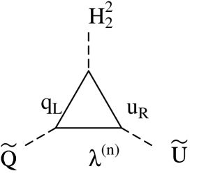
Figure 3: Diagrams contributing to $A_{t}$

and given by

$$A_{t}=\frac{2\alpha_{3}h_{t}}{3\pi^{2}R}\left[iLi_{2}\left(e^{2\pi i\omega}\right)-i\left(e^{-2\pi i\omega}\right)\right]$$ (3.77)

Supersymmetry breaking is then gauge and Yukawa mediated to the bosonic fields of the chiral sector localized on the branes by radiative corrections. In this aspect the model shares common features with any gauge mediated supersymmetry breaking model but with a very characteristic spectrum. Electroweak symmetry breaking is also easily triggered by radiative corrections at one-loop if the top is living in the bulk [26]. In fact the tachyonic mass induced by the top Yukawa coupling is also finite [26].

The fact that the radiative contributions to soft masses are finite does not mean that they are not sensitive to the ultraviolet cut-off at any order of perturbation theory. It just means that there is no mass counter-term at any order in perturbation theory. An explicit dependence on the cut-off already appears in the two-loop correction to the soft masses [29]. However it comes exclusively from the wave function renormalization and can be absorbed in the redefinition the gauge and Yukawa couplings in the improved theory. In fact the wave function renormalization yields a renormalization of gauge and Yukawa couplings that contains a power-law dependence on the cut-off. This power law renormalization [31] has led to the possibility of power-law or accelerated unification [32] in the TeV range that parallels the ordinary logarithmic unification in the MSSM .

3.3 Supersymmetry breaking by Hosotani mechanism

In the five dimensional formulation of local supersymmetry the $SU(2)_{R}$ global supersymmetry is promoted to a local symmetry [34, 35, 36]. This subject is being extensively studied at present. We will use the formulation of Ref. [34] where two multiplets are necessary to formulate off-shell five dimensional supergravity: the minimal supergravity multiplet $(40_{B}+40_{F})$ and the tensor multiplet $(8_{B}+8_{F})$. Their parities are given in tables 6 and 7, respectively.

Table 6: Minimal supergravity multiplet

Field		$Z=+1$	$Z=-1$
$g_{MN}$	graviton	$g_{\mu\nu}$, $g_{55}$	$g_{\mu 5}$
$\psi_{M}$	gravitino	$\psi^{1}_{\mu L}$, $\psi^{2}_{5L}$	$\psi^{2}_{\mu L}$, $\psi^{1}_{5L}$
$B_{M}$	graviphoton	$B_{5}$	$B_{\mu}$
$\vec{V}_{M}$	$SU(2)_{R}$-gauge	$V_{\mu}^{3}$, $V_{5}^{1,2}$	$V_{5}^{3}$, $V_{\mu}^{1,2}$
$v^{MN}$	antisymmetric	$v^{\mu 5}$	$v^{\mu\nu}$
$\vec{t}$	$SU(2)_{R}$-triplet	$t^{1,2}$	$t^{3}$
$C$	real scalar	$C$
$\zeta$	$SU(2)_{R}$-doublet	$\zeta^{1}_{L}$	$\zeta^{2}_{L}$

Table 7: Tensor multiplet

Field	$Z=+1$	$Z=-1$
$\vec{Y}$	$Y^{1,2}$	$Y^{3}$
$B_{MNP}$	$B_{\mu\nu\rho}$	$B_{\mu\nu 5}$
$N$	$N$
$\rho$	$\rho^{1}_{L}$	$\rho^{2}_{L}$

Fields in the upper panel of table 6 are physical fields while those in the lower panel are auxiliary fields. Fields in table 7 are all of them auxiliary fields.

The $SU(2)_{R}$ gauge fixing is done by fixing the compensator field [34]

$$\vec{Y}=e^{u}\,\left(\begin{array}[]{c}0\\ 1\\ 0\end{array}\right)$$ (3.78)

that breaks $SU(2)_{R}\to U(1)_{R}=\{\sigma^{2}\}$. The invariant Lagrangian $\mathcal{L}_{grav}=\mathcal{L}_{minimal}+\mathcal{L}_{tensor}$ contains the term $(1-e^{u})C$ and then the equation of motion of $C$ yields $u=0$.

The auxiliary fields that are relevant for supersymmetry breaking are: $V_{5}^{1,2},\ t^{1,2}$, that constitute the $F$-term of the radion superfield [37, 38, 39, 40],

$$\mathcal{R}=\left[g_{55}+iB_{5},\psi^{2}_{5L},V_{5}^{1}+i\,V_{5}^{2}+4i\,(t^{1}+i\,t^{2})\right]$$ (3.79)

The relevant terms in $\mathcal{L}_{grav}$ containing these fields are [34]

$$\mathcal{L}_{grav} = -\frac{i}{2}\bar{\psi}_{P}\gamma^{PMN}\mathcal{D}_{M}\psi_{N}-\frac{1}{12}\epsilon^{MNPQR}V_{M}^{2}\partial_{N}B_{PQR}$$ (3.80)

$$+ (V^{1}_{5})^{2}-12(t^{1})^{2}-48(t^{2})^{2}-12N\,t^{2}-N^{2}$$

where $\gamma^{PMN}$ is the normalized antisymmetric product of gamma matrices,

$$\mathcal{D}_{M}=D_{M}+i\sigma^{2}V_{M}^{2}$$ (3.81)

and $D_{M}$ is the covariant derivative with respect to local Lorentz transformations. The field equations for the auxiliary fields yield

$$V^{1}_{5}=N=t^{1}=t^{2}=0$$ (3.82)

while the field equation for the 3-form tensor $B_{MNP}$ gives

$$\partial_{\left[M\right.}V^{2}_{\left.N\right]}=0\Longrightarrow V^{2}_{M}=\partial_{M}K\Longrightarrow\left\{\begin{array}[]{l}V^{2}_{\mu}=0\ ({\rm odd\ field})\\ V_{5}^{2}={\rm constant}\ ({\rm even\ field})\end{array}\right.$$ (3.83)

where $K$ is an odd field and the last implication is suggested by the simplest choice

$$K=y\,\frac{\omega}{R}$$ (3.84)

which leads to the background

$$V^{2}_{5}=\frac{\omega}{R}$$ (3.85)

and makes the connection between the Hosotani/Wilson picture and the Scherk-Schwarz one. In fact using the coupling of $V^{2}_{5}$ to the gravitino field through the covariant derivative $\mathcal{D}_{5}$ in (3.80) one obtains the gravitino mass eigenvalues for the Kaluza-Klein modes as

$$m_{3/2}^{(n)}=\frac{n+\omega}{R}$$ (3.86)

An alternative choice to the odd function (3.84) has been proposed in Refs. [24, 41] as

$$K=\Lambda_{1}\delta(y)+\Lambda_{2}\delta(y-\pi R)$$ (3.87)

that leads, through the covariant derivative $\mathcal{D}_{5}$ in (3.80), to a localized gravitino mass term. In this case the gravitino modes mass matrix has to be diagonalized and mass eigenstates computed. The resulting spectrum is similar to that in Eq. (3.86) thus proving that supersymmetry breaking by a localized gravitino mass (that can arise e. g. from some non-perturbative dynamics) is equivalent to a global Scherk-Schwarz breaking, as anticipated in Ref. [42]. The issue of supersymmetry breaking by a localized mass on the brane will the subject of section 3.3.3.

Supersymmetry breaking is also manifest for gauginos and hyperscalars, $SU(2)_{R}$ doublets, that interact with $\vec{V}_{M}$ through the covariant derivative, see Eq. (2.29)

$$\mathcal{L}_{matter}=\frac{i}{2}\bar{\lambda}\gamma^{M}\widehat{\mathcal{D}}_{M}\lambda+\left|\widehat{\mathcal{D}}_{M}A\right|$$ (3.88)

where

$$\widehat{\mathcal{D}}_{M}=D_{M}+i\,\vec{\sigma}\cdot\vec{V}_{M}$$ (3.89)

After using the equations of motion $V^{1,3}_{5}=0$ we obtain that $\widehat{\mathcal{D}}_{M}\to\mathcal{D}_{M}$ and the mass eigenvalues for gauginos and hyperscalars are, as for gravitinos,

$$m_{1/2}^{(n)}=m_{0}^{(n)}=\frac{n+\omega}{R}$$ (3.90)

which also shows the equivalence between the Hosotani/Wilson mechanism and the Scherk-Schwarz compactification for the matter sector.

Supersymmetry breaking is spontaneous provided there is a (massless) Goldstone fermion (Goldstino) “eaten” by the gravitino that becomes massive in the unitary gauge. This is known as the super-Higgs effect [43] and will be considered next.

3.3.1 Super-Higgs effect

The Goldstino is provided by the fifth component of the gravitino: $\psi_{5}$. This is obvious from the local supersymmetry transformation,

$$\delta_{\xi}\psi_{5}=\mathcal{D}_{5}\xi+\cdots=i\sigma^{2}\,V^{2}_{5}\xi+\cdots$$ (3.91)

We will now analyze the corresponding super-Higgs effect [40]. The kinetic term for the gravitino can be decomposed in four-dimensional and extra-dimensional components as:

$$-\frac{i}{2}\bar{\psi}_{M}\gamma^{MNP}\mathcal{D}_{N}\psi_{P} = -\frac{i}{2}\bar{\psi}_{\mu}\gamma^{\mu\nu\rho}\mathcal{D}_{\nu}\psi_{\rho}+\frac{i}{2}\bar{\psi}_{\mu}\gamma^{\mu\nu}\gamma^{5}\mathcal{D}_{5}\psi_{\nu}$$ (3.92)

$$- \frac{i}{2}\bar{\psi}_{\mu}\gamma^{\mu\nu}\gamma^{5}\mathcal{D}_{\nu}\psi_{5}-\frac{i}{2}\bar{\psi}_{5}\gamma^{\mu\nu}\gamma^{5}\mathcal{D}_{\mu}\psi_{\nu}$$

We can now make the redefinition

$$\psi_{\mu}=\psi^{\prime}_{\mu}+\mathcal{D}_{\mu}(\mathcal{D}_{5})^{-1}\psi_{5}$$ (3.93)

which can be seen as a local supersymmetry transformation with parameter $(\mathcal{D}_{5})^{-1}\psi_{5}\equiv\xi$, gauging $\psi_{5}$ away. This defines a “super-unitary” gauge where $\psi_{5}$ has been “eaten” by the four dimensional gravitino $\psi_{\mu}$:

$$-\frac{i}{2}\bar{\psi}_{M}\gamma^{MNP}\mathcal{D}_{N}\psi_{P} = -\frac{i}{2}\epsilon^{\mu\nu\rho\sigma}\bar{\psi}^{\prime}_{\mu}\gamma_{\sigma}\gamma^{5}\mathcal{D}_{\nu}\psi^{\prime}_{\rho}$$ (3.94)

$$+ \frac{i}{2}\psi^{\prime}_{\mu}\gamma^{\mu\nu}\gamma^{5}\left(\partial_{5}+i\,\frac{\omega}{R}\sigma^{2}+\cdots\right)\psi^{\prime}_{\nu}$$

The second term of (3.94) provides a mass term for the four dimensional gravitino as

$$\mathcal{L}_{mass}=\frac{1}{2}\left(\begin{array}[]{cc}\psi^{1}_{\mu\,L}&\psi^{2}_{\mu\,L}\end{array}\right)\sigma^{\mu\nu}\left(\begin{array}[]{cc}\frac{\omega}{R}&ip_{5}\\ -ip_{5}&\frac{\omega}{R}\end{array}\right)\left(\begin{array}[]{c}\psi^{1}_{\nu\,L}\\ \psi^{2}_{\nu\,L}\end{array}\right)+h.c.$$ (3.95)

where $p_{5}\equiv i\partial_{5}=n/R$ for a flat (unwarped) extra dimension and $\omega$ is defined as a function of the background field $V^{2}_{5}$ in Eq. (3.85). The eigenvalues of the mass matrix (3.95) are $|n\pm\omega|/R$ in agreement with Eq. (3.86).

3.3.2 Radiative determination of the Scherk-Schwarz parameter

The effective potential along the $V^{2}_{5}$, i. e. $\omega$, direction is flat and hence the Scherk-Schwarz parameter is undetermined at the tree-level. The scale of supersymmetry breaking (i. e. the gravitino mass) also is undetermined at the tree-level, a situation which is typical of no-scale models in supergravity [44].

Since all mass eigenvalues, for gravitinos, gauginos and hyperscalars, are equal to (3.86) we can compute the Coleman-Weinberg [45] one-loop effective potential in the following way. For hyperscalars we have

$$V_{0}=\frac{2N_{H}}{2}\sum_{n=-\infty}^{\infty}\int\frac{d^{4}p}{(2\pi)^{4}}\log\left[p^{2}+\left(\frac{n+\omega}{R}\right)^{2}\right]$$ (3.96)

where $2N_{H}=2$ (# degrees of freedom of a complex scalar)$\times N_{H}$ (# of hypermultiplets)$\times 2$ (# scalars in one hypermultiplet)$\times 1/2$ (orbifold reduction of # degrees of freedom). Similarly for gauginos we get

$$V_{1/2}=-\frac{2N_{V}}{2}\sum_{n=-\infty}^{\infty}\int\frac{d^{4}p}{(2\pi)^{4}}\log\left[p^{2}+\left(\frac{n+\omega}{R}\right)^{2}\right]$$ (3.97)

where the minus sign comes from the fermionic character of gauginos and $N_{V}$ is the number of vector multiplets, while for the gravitino, in the five dimensional harmonic gauge $\gamma^{N}\psi_{N}=0$ the effective potential is easily worked out to be [46]

$$V_{3/2}=-\frac{4}{2}\sum_{n=-\infty}^{\infty}\int\frac{d^{4}p}{(2\pi)^{4}}\log\left[p^{2}+\left(\frac{n+\omega}{R}\right)^{2}\right]$$ (3.98)

Using techniques from field theory at finite temperature one obtains [26]

$$V_{eff}=\frac{3(2+N_{V}-N_{H})}{64\pi^{6}R^{4}}\left[Li_{5}\left(e^{2\pi i\omega}\right)+h.c.\right]$$ (3.99)

where the polylogarithm functions are defined in Eq. (3.75), and $Li_{5}$ has a power expansion as

$$Li_{5}\left(e^{2\pi i\omega}\right)+h.c.=2\zeta(5)-4\pi^{2}\zeta(3)\omega^{2}+\cdots$$ (3.100)

Moreover using the expansion (3.100) it is easy to see that the global minimum of the potential is $\omega=0$ ($\omega=1/2$) for $N_{H}>2+N_{V}$ ($N_{H}<2+N_{V}$). This value can be shifted if there is another source of supersymmetry breaking; for instance if the Scherk-Schwarz breaking is “assisted” by brane effects, as we will see in the next section.

3.3.3 Brane assisted Scherk-Schwarz supersymmetry breaking

The coupling of the minimal and tensor multiplets to the branes permits a total Lagrangian as

$$\mathcal{L}=\mathcal{L}_{grav}+2\,W\delta(y)\mathcal{L}_{brane}$$ (3.101)

with [34, 47]

$$\mathcal{L}_{brane}=-2\,N-2\,V^{1}_{5}-12\,t^{2}+\frac{1}{2}\,\bar{\psi}_{\mu}\sigma^{2}\gamma^{\mu\nu}\psi_{\nu}$$ (3.102)

Where we can always assume that $W$ comes from some non-perturbative dynamics that appears when some brane fields in the hidden sector are integrated out. This typically happens when supersymmetry is broken by gaugino condensation, as it is the case in $M$-theory [42, 48]. Of course in general one could also introduce another term localized at the other brane, as $2\,W^{\prime}\delta(y-\pi R)$, but we will work out here the simplest case.

In the presence of brane terms the field equations of the auxiliary fields $N$ and $V^{1}_{5}$ are modified to

$$N=-2\,W\delta(y),\quad V^{1}_{5}=2\,W\delta(y).$$ (3.103)

The presence of these VEV’s modify the mass terms [49] for gauginos,

$$\mathcal{M}_{1/2}=i\gamma^{5}\widetilde{\mathcal{D}}_{5}=i\gamma^{5}\left(\partial_{5}+i\sigma^{1}V_{5}^{1}+i\sigma^{2}V_{5}^{2}\right)$$ (3.104)

and hyperscalars,

$$\mathcal{M}_{0}^{2}=\widetilde{\mathcal{D}}_{5}\widetilde{\mathcal{D}}^{5}$$ (3.105)

while the gravitino mass is directly modified by the term in $\mathcal{L}_{brane}$:

$$2\,W\delta(y)\,\frac{1}{2}\,\bar{\psi}_{\mu}\gamma^{\mu\nu}\sigma^{2}\psi_{\nu}$$ (3.106)

The corresponding mass eigenvalues can be seen to be modified by the presence of $W\neq 0$ as [49]

$$m^{(n)}_{a}=\frac{n+\Delta_{a}(\omega,W)}{R},\quad a=0,\ 1/2,\ 3/2$$ (3.107)

where the quantities $\Delta_{a}(\omega,W)$ have been computed to be [24]

$$\Delta_{3/2}(\omega,W) = \arctan\sqrt{\frac{\tan^{2}(\omega\pi)+\tanh^{2}(W)}{1+\tan^{2}(\omega\pi)\,\tanh^{2}(W)}}$$

$$\Delta_{1/2,0}(\omega,W) = \arctan\sqrt{\frac{\tan^{2}(\omega\pi)+\tan^{2}(W)}{1+\tan^{2}(\omega\pi)\,\tan^{2}(W)}}$$ (3.108)

The modified mass eigenvalues produce a modification of the effective potential that turns out to be [49]

$$V_{\rm eff} = \frac{3}{36\pi^{6}R^{4}}\left[Li_{5}\left(e^{2\pi i\Delta_{3/2}(\omega,W)}\right)+h.c.\right]$$

$$+ \frac{3(N_{V}-N_{H})}{64\pi^{6}R^{4}}\left[Li_{5}\left(e^{2\pi i\Delta_{1/2}(\omega,W)}\right)+h.c.\right]$$

We expect that the brane effects can modify continuously the location of the minimum of the effective potential away from its minima for $W=0$ at $\omega=0$ and $\omega=1/2$. We have studied numerically two extreme cases. First of all, the case where only the gravitational and gauge sectors are living in the bulk of the extra dimension, while matter and Higgs fields are localized in the observable brane. This case, that corresponds to $N_{V}=12$ and $N_{H}=0$, is shown in Fig. 4.

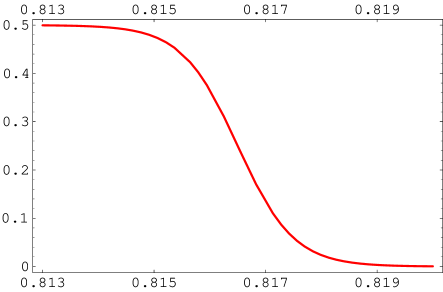
Figure 4: Plot of the minimum of the effective potential $\omega_{min}$ as a function of $W$ for $N_{V}=12$ and $N_{H}=0$

We can see that for $W=0$ the minimum of the potential is $\omega_{min}=1/2$ while for $W\stackrel{{\scriptstyle>}}{{{}_{\sim}}}0.82$ it smoothly becomes $\omega_{min}=0$ with a smooth transition region around $W\simeq 0.815$. Finally we have considered the other extreme case where all gravitational, gauge, matter and Higgs fields are propagating in the bulk of the extra dimensions, which amounts to considering the case with $N_{V}=12$ and $N_{H}=49$. This case is shown in Fig. 5.

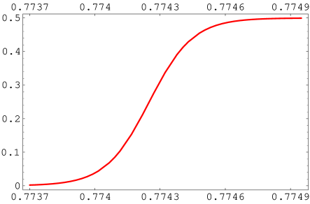
Figure 5: Plot of the minimum of the effective potential $\omega_{min}$ as a function of $W$ for $N_{V}=12$ and $N_{H}=49$

We can see from Fig. 5 that for $W=0$ the minimum of the potential is $\omega_{min}=0$ while for $W\stackrel{{\scriptstyle>}}{{{}_{\sim}}}0.775$ it becomes $\omega_{min}=1/2$ with a smooth transition region around $W\simeq 0.774$.

4 Gauge symmetry breaking

In this section we will consider the different mechanisms of gauge symmetry breaking based on the existence of extra dimensions. As we did in section 3, in order to simplify the analysis we will concentrate on a five-dimensional theory, i. e. $d=1$, where the extra dimension is compactified on the orbifold $S^{1}/\mathbb{Z}_{2}$. As we will see we can use both the orbifold (section 4.1) and Scherk-Schwarz (section 4.2) boundary conditions to break the gauge symmetry on the boundaries. Moreover if bulk fermions strongly coupled to the Higgs (i. e. the top quark) propagate in the bulk of the extra dimensions they induce a spontaneous one-loop (Coleman-Weinberg) finite electroweak breaking as we will describe in some detail in section 4.3.

4.1 Gauge breaking by orbifolding

In section 3.1 we have (almost) always been assuming that the orbifold action was commuting with the gauge structure and so the gauge group remained intact after orbifolding. This is clearly not the most general case for the orbifold action can break the gauge group $\mathcal{G}$ in the bulk into its subgroup $\mathcal{H}$ on the branes. This breaking must be consistent with the orbifold action and so it is strongly constrained. Here we will consider the case of a general gauge group with breaking $\mathcal{G}\to\mathcal{H}$ by the $\mathbb{Z}_{2}$ projection.

We consider gauge fields $A_{M}=A_{M}^{A}T^{A}$ where $T^{A}$ are the Lie algebra generators of $\mathcal{G}$ normalized such that

$${\rm tr}\left\{T^{A}T^{B}\right\}=\frac{1}{2}\,\delta^{AB}$$ (4.1)

with indices $M=\mu,5$ and $A=1,\cdots,dim(\mathcal{G})$. We couple to the gauge fields Dirac spinors $\psi$ that transform in the representation $\underline{R}$ [with $dim(\underline{R})\equiv d_{R}$] of the group $\mathcal{G}$.

The five dimensional action can be written as

$$S_{5}=\int d^{5}x\ {\rm Tr}\,\left\{-\frac{1}{2}F_{MN}F^{MN}+i\bar{\psi}\gamma^{M}D_{M}\psi\right\}$$ (4.2)

where $F_{MN}=F_{MN}^{A}T^{A}$, $F_{MN}^{A}=\partial_{M}A_{N}^{A}-\partial_{N}A_{M}^{A}+gf^{ABC}A_{M}^{B}A_{N}^{C}$ and the gauge covariant derivative is $D_{M}=\partial_{M}-igA_{M}^{A}T_{R}^{A}$, where $T_{R}^{A}$ are Lie-algebra valued matrices in the representation $\underline{R}$ of $\mathcal{G}$ satisfying

$$\left[T_{R}^{A},T_{R}^{B}\right]=if^{ABC}T_{R}^{C}.$$ (4.3)

The $\mathbb{Z}_{2}$ parity assignment is defined as

$$A_{M}^{A}(x^{\mu},-y) = \alpha^{M}\Lambda^{AB}A^{B}_{M}(x^{\mu},y)$$

$$\psi(x^{\mu},-y) = \lambda_{R}\otimes(i\gamma^{5})\,\psi(x^{\mu},y)$$ (4.4)

where $\alpha^{\mu}=+1$ and $\alpha^{5}=-1$, which just means that the parities of $A^{A}_{\mu}$ and $A_{5}^{A}$ are opposite, and $\lambda_{R}=\lambda_{R}^{\dagger}=\lambda_{R}^{-1}$ is a matrix acting on the representation indices of $\psi$. Finally $\Lambda^{2}=1$ and so its eigenvalues are $\pm 1$.

By imposing the requirement that under the $\mathbb{Z}_{2}$ action $F_{MN}^{A}\to\alpha^{M}\Lambda^{AB}F_{MN}^{B}$, and that $F_{MN}^{A}F_{MN}^{A}$ remains invariant it is straightforward to check that $\Lambda^{AB}$ should satisfy the condition [50]

$$f^{ABC}=\Lambda^{AA^{\prime}}\Lambda^{BB^{\prime}}\Lambda^{CC^{\prime}}f^{A^{\prime}B^{\prime}C^{\prime}}$$ (4.5)

which implies that the action of $\mathbb{Z}_{2}$ on the Lie-algebra of $\mathcal{G}$ is a Lie-algebra automorphism .

With no loss of generality we can consider the diagonal basis where $\Lambda^{AA^{\prime}}=\eta^{A}\delta^{AA^{\prime}}$ with $\eta^{A}=\pm 1$ and the automorphism condition (4.5) takes the simpler form

$$f^{ABC}=\eta^{A}\eta^{B}\eta^{C}f^{ABC}\quad{\rm(no\ sum)}$$ (4.6)

Using now the $\mathbb{Z}_{2}$ action (4.6) we can naturally split the adjoint index $T^{A}$ into an unbroken part $T^{a}$ ($\eta^{a}=+1$) and a broken part $T^{\hat{a}}$ ($\eta^{\hat{a}}=-1$) such that $\mathcal{H}=\{T^{a}\}$, $\mathcal{K}=\mathcal{G}/\mathcal{H}=\{T^{\hat{a}}\}$. In this way the parities of gauge bosons are given in table 8.

Table 8: Parities of gauge sector

EVEN	$A_{\mu}^{a}$	$A_{5}^{\hat{a}}$
ODD	$A_{\mu}^{\hat{a}}$	$A_{5}^{a}$

Following table 8 only $A_{\mu}^{a}$ and $A_{5}^{\hat{a}}$ contain zero-modes and are non-vanishing on the branes. In particular $A_{\mu}^{a}$ are the gauge bosons on the brane corresponding to the gauge group $\mathcal{H}$ and $A_{5}^{\hat{a}}$ are massless scalars on the brane. When the latter acquire a VEV they can spontaneously break the gauge group $\mathcal{H}$ to a subgroup, a mechanism known as the Hosotani mechanism [12]. This will be discussed later on in section 4.2.

The automorphism constraint (4.5) implies that the only non-vanishing structure constants are $f^{abc}$ and $f^{a\hat{b}\hat{c}}$, which strongly constrains the possible breakings. A trivial example where we can see that the automorphism constraint is a non-trivial one is the case $\mathcal{G}=SU(2)$. Its only non-vanishing structure constant is $f^{123}=\varepsilon^{123}$ (and permutations thereof). There are thus only two possibilities:

• The case $a=1,2,3$, which corresponds to no breaking: $\mathcal{H}=SU(2)$.

• The case $a=3$ and $\hat{a}=1,2$, which corresponds to the breaking $SU(2)\to U(1)$.

In particular we can easily check that the breaking $SU(2)\to$ nothing is not allowed by the orbifold action.

As for fermions $\psi$ in the representation $R$ of the group $\mathcal{G}$, the requirement that the fermion-gauge boson coupling $igA^{A}_{M}\bar{\psi}\gamma^{M}T^{A}\psi$ is invariant under the orbifold action implies that the matrix $\lambda_{R}$ in (4.1) should satisfy the condition [51]

$$\lambda_{R}T^{A}_{R}\lambda_{R}=\eta^{A}T^{A}_{R}\Longrightarrow\left\{\begin{array}[]{c}\left[\lambda_{R},T^{a}_{R}\right]=0\\ \\ \left\{\lambda_{R},T^{\hat{a}}_{R}\right\}=0\end{array}\right.$$ (4.7)

The final issue here is the gauge-fixing term and ghost Lagrangian

$$\mathcal{L}_{g.f.}+\mathcal{L}_{ghost}=-\frac{1}{2\xi}\partial^{M}A_{M}^{A}\,\partial^{M}A_{M}^{A}+{\rm Tr}\,\partial^{M}\bar{c}D_{M}c$$ (4.8)

A quick glance at the ghost-gauge field interactions shows that ghosts $c^{A}$ have the same parity properties as the gauge fields $A_{\mu}^{A}$ in (4.1), i. e.

$$c^{A}(x^{\mu},-y)=\Lambda^{AB}c^{B}(x^{\mu},y)$$ (4.9)

Finally we would like to comment that the Lie-algebra automorphisms come in two classes that will be subsequently analyzed:

• Inner automorphisms, that can be written as a group conjugation: $T^{A}\to gT^{A}g^{-1}$, $g\in\mathcal{G}$. Inner automorphisms preserve the rank $\Rightarrow$ $rank(\mathcal{H})=rank(\mathcal{G})$.

• Outer automorphisms, that can not be written as a group conjugation and therefore do not preserve the rank $\Rightarrow$ $rank(\mathcal{H})<rank(\mathcal{G})$.

4.1.1 Rank preserving orbifold breaking

The case $rank(\mathcal{H})=rank(\mathcal{G})$ implies that none of the generators $T_{R}^{\hat{a}}$ are diagonal and therefore $\lambda_{R}$ can be chosen diagonal

$$\lambda_{R}=\left(\begin{array}[]{cc}{\sf I}{\rm 1}_{d_{1}}&0\\ 0&-{\sf I}{\rm 1}_{d_{2}}\end{array}\right)$$ (4.10)

where $d_{1}$ and $d_{2}$ are model dependent numbers.

The general structure for rank preserving orbifolding is better presented in the Cartan-Weyl basis for the generators $T^{A}$. In this basis the generators are organized into the Cartan subalgebra generators $H_{i}$, $i=1,\cdots,rank(\mathcal{G})$, and “raising” and “lowering” generators $E_{\alpha}$, $\alpha=1,\cdots,\,dim(\mathcal{G})-rank(\mathcal{H})$ with

$$\left[H_{i},E_{\alpha}\right]=\alpha_{i}E_{\alpha}$$ (4.11)

where the $rank(\mathcal{G})$-dimensional vector $\vec{\alpha}$ is the root associated to $E_{\alpha}$ [52]. The orbifold action on gauge fields can be written as the group conjugation

$$T^{A}\to g\,T^{A}\,g^{-1},\quad{\rm with}\quad g=e^{-2\pi i\vec{v}\cdot\vec{H}}$$ (4.12)

The orbifold action is then fully specified by the $rank(\mathcal{G})$-dimensional twist vector $\vec{v}$. Using now standard commutation relations it can be verified that

$$g\,E_{\alpha}\,g^{-1} = e^{-2\pi i\vec{v}\cdot\vec{\alpha}}E_{\alpha}$$ (4.13)

$$g\,H_{i}\,g^{-1} = H_{i}$$ (4.14)

From the last equality it follows that the inner automorphism (4.12) preserves the rank. Moreover $E_{\alpha}$ generators with roots $\vec{\alpha}$ such that $\vec{\alpha}\cdot\vec{v}=0$ belong to the unbroken subgroup. The problem of determining the unbroken subgroup is thus reduced to an algebraic problem, as we will see next in some examples.

$SU(2)\to U(1)$ example

This is the simplest non-trivial example. We have already seen that the only non-trivial $SU(2)$ breaking corresponds to $SU(2)\to U(1)$ by the $\Lambda^{AB}$ matrix

$$\Lambda=\left(\begin{array}[]{ccc}-1&0&0\\ 0&-1&0\\ 0&0&+1\end{array}\right)$$ (4.15)

In the Cartan-Weyl basis: $H_{1}=T^{3}$, $E_{\pm}=T^{1}\pm i\,T^{2}$, with the non-zero roots $\alpha_{\pm}=\pm 1$ and the commutation rules

$$\left[H_{1},E_{\pm}\right]=\pm E_{\pm}$$ (4.16)

The unbroken $U(1)$ corresponds to the generator $H_{1}$. The orbifold breaking (4.15) is triggered by the twist vector $v=-\frac{1}{2}$ and the group element

$$g=e^{i\pi T^{3}}$$ (4.17)

Fermions in this example will be considered in the fundamental representation $R=\underline{2}$. One can easily see that

$$\lambda_{\underline{2}}=\pm\left(\begin{array}[]{cc}1&0\\ 0&-1\end{array}\right),$$ (4.18)

i. e. $d_{1}=d_{2}=1$ in the notation of (4.10). In fact $\lambda_{\underline{2}}$ in (4.18) commutes with $T^{a}=T^{3}=\frac{1}{2}\sigma^{3}$ and anti-commutes with $T^{\hat{a}}=\left\{T^{1}=\frac{1}{2}\sigma^{1},T^{2}=\frac{1}{2}\sigma^{2}\right\}$ in agreement with the general orbifold condition (4.7). The surviving fermions on the brane are left-handed fermions with $U(1)$-charge equal to $+1$ and right-handed fermions with $U(1)$-charge equal to $-1$, and so the fermion spectrum in the bulk is non-chiral.

$SU(3)\to SU(2)\otimes U(1)$ example

The next to simplest example of orbifold breaking by an inner automorphism corresponds to $SU(3)\to SU(2)\otimes U(1)$. In order to achieve this breaking pattern we take the $\Lambda^{AB}$ matrix as

$$\Lambda=\left(\begin{array}[]{ccc}{\sf I}{\rm 1}_{3}&0&0\\ 0&-{\sf I}{\rm 1}_{4}&0\\ 0&0&+{\sf I}{\rm 1}_{1}\end{array}\right)$$ (4.19)

so that the $SU(3)$ generators [see Eq. (4.33)] corresponding to $SU(2)\otimes U(1)$ have positive parity and those corresponding to $SU(3)/SU(2)\otimes U(1)$ negative parity. In the Cartan-Weyl basis we have four unbroken generators: the Cartan generators $H_{1},\,H_{2}$, and two other unbroken generators $E_{\pm 1}$ corresponding to the roots $\vec{\alpha}_{\pm 1}=(\pm 1,0)$. The twist is $\vec{v}=(0,\sqrt{3})$ and so $\vec{\alpha}_{\pm 1}\cdot\vec{v}=0$. For the rest of generators $E_{\pm 2},\,E_{\pm 3}$ we find $\exp(-2\pi i\vec{v}\cdot\vec{\alpha})=-1$ as expected.

Choosing fermions in the representation $R=\underline{3}$ we find $\lambda_{\underline{3}}=\pm diag(+1,+1,-1)$ that commutes with the generators of $SU(2)\otimes U(1)$ and anti-commute with those of $SU(3)/SU(2)\otimes U(1)$. Using now the decomposition $\underline{3}=\underline{2}_{\,-1}\oplus\underline{1}_{\,+2}$ we obtain on the brane a massless $SU(2)$ doublet with a given chirality and a massless $SU(2)$ singlet with opposite chirality. The spectrum is chiral and anomaly cancellation must be enforced in this model.

A classification of breaking patterns by $\mathbb{Z}_{2}$ inner automorphisms is given in table 9. For more details see Ref. [50].

Table 9: Breaking pattern by inner automorphisms

$\mathcal{G}$	$\mathcal{H}$
$SU(p+q)$	$SU(p)\otimes SU(q)\otimes U(1)$
$SO(p+q)$	$SO(p)\otimes SO(q)$, $p$ or $q$ even
$SO(2n)$	$SU(n)\otimes U(1)$
$E_{6}$	$SU(6)\otimes SU(2)$, $SO(10)\otimes U(1)$

Final remarks

Rank preservation by inner automorphisms holds for arbitrary $\mathbb{Z}_{N}$ (abelian) orbifolds. For non-abelian orbifolds the group element $g$ can not in general be written as $\exp\{-2\pi i\vec{v}\cdot\vec{H}\}$ and therefore group conjugation can act non-trivially on some $H_{i}$ leading to the projection of the corresponding gauge fields and thus to rank lowering. However considering non-abelian orbifolds is too complicated a way of achieving rank lowering for a simpler way of doing it does exist in the $\mathbb{Z}_{N}$ orbifolds when the discrete group is not realized as a group conjugation, as we will see in the next section.

4.1.2 Rank lowering

If the discrete group in Eq. (4.1) can not be realized as the group conjugation (4.12) its action on the Lie algebra is called an outer automorphism and leads to rank reduction. In short, outer automorphisms are structure constant preserving linear transformations of the generators that can not be written as a group conjugation. For any given Lie algebra there is only a limited number of outer automorphisms depending on the symmetries of the Dynkin diagrams.

Reduced rank implies that some of the $T_{R}^{\hat{a}}$ are diagonal and for them the identity $\{\lambda_{R},T_{R}^{\hat{a}}\}=0$ can never be satisfied if $\lambda_{R}$ is diagonal. The most interesting case is

$$\Lambda^{AB}T_{R}^{B}=-\left(T_{R}^{A}\right)^{T}$$ (4.20)

which of course preserves the structure constants. This is an outer automorphism that produces the breaking $SU(N)\to SO(N)$. In this case we must find a non-diagonal (and unitary) matrix in the $R$-representation, $\lambda_{R}$, that solves Eqs. (4.7), i. e.

$$\lambda_{R}T_{R}^{A}\lambda_{R}=-\left(T_{R}^{A}\right)^{T}$$ (4.21)

This identity can only be satisfied if $R$ is a real representation. In fact one can always choose $R=\mathcal{R}\oplus\bar{\mathcal{R}}$ where $\mathcal{R}$ is a non-real representation with generators

$$T_{R}^{A}=\left(\begin{array}[]{cc}T_{\mathcal{R}}^{A}&0\\ 0&-\left(T_{\mathcal{R}}^{A}\right)^{T}\end{array}\right)$$ (4.22)

which implies that $\lambda_{R}$ takes the block form

$$\lambda_{R}=\left(\begin{array}[]{cc}0&{\sf I}{\rm 1}_{\mathcal{R}}\\ {\sf I}{\rm 1}_{\mathcal{R}}&0\end{array}\right)$$ (4.23)

and so it has $d_{\mathcal{R}}$ eigenstates $(\hat{e}_{i},\hat{e}_{i})$ with positive parity and $d_{\mathcal{R}}$ eigenstates $(\hat{e}_{i},-\hat{e}_{i})$ with negative parity, where $\hat{e}_{i}$ denotes the usual unit vector with a unit in the $i$-th entry and zero otherwise.

The zero-mode spectrum resulting from this action will always be vector like and therefore anomaly-free. To produce a chiral theory the simplest possibility would be to add chiral, anomaly-free, matter of the $\mathcal{H}$ subgroup localized on the brane where $\mathcal{G}\to\mathcal{H}$ via the outer automorphism. Explicit examples will be presented next.

$U(1)\to nothing\quad$ example

The simplest example is $U(1)$ in the bulk breaking down to nothing on the branes. The choice that performs this breaking is $\Lambda=-1$, that is a simple realization of the equation $\Lambda\,T=-T^{T}$, with $T=1$. Charged fermions are necessarily accompanied by oppositely charged partners. The fermionic zero mode spectrum is a vector-like pair of Weyl fermions that can be assembled into a Dirac fermion.

$SU(3)\to SO(3)$ example

The second simplest example of an automorphism with rank breaking action is $SU(3)\to SO(3)$. Solving equation (4.20) one must give a positive parity to antisymmetric generators and a negative parity to symmetric ones. In particular the generators for the $SU(3)$ group are given by the Gell-Man matrices:

$$\lambda^{1} = \frac{1}{2}\left(\begin{array}[]{ccc}0&1&0\\ 1&0&0\\ 0&0&0\\ \end{array}\right)\quad\lambda^{2}=\frac{1}{2}\left(\begin{array}[]{ccc}0&-i&0\\ i&0&0\\ 0&0&0\\ \end{array}\right)\quad\lambda^{3}=\frac{1}{2}\left(\begin{array}[]{ccc}1&0&0\\ 0&-1&0\\ 0&0&0\\ \end{array}\right)\quad$$ (4.33)

$$\lambda^{4} = \frac{1}{2}\left(\begin{array}[]{ccc}0&0&1\\ 0&0&0\\ 1&0&0\\ \end{array}\right)\quad\lambda^{5}=\frac{1}{2}\left(\begin{array}[]{ccc}0&0&-i\\ 0&0&0\\ i&0&0\\ \end{array}\right)$$ (4.40)

$$\lambda^{6} = \frac{1}{2}\left(\begin{array}[]{ccc}0&0&0\\ 0&0&1\\ 0&1&0\\ \end{array}\right)\quad\lambda^{7}=\frac{1}{2}\left(\begin{array}[]{ccc}0&0&0\\ 0&0&-i\\ 0&i&0\\ \end{array}\right)\quad\lambda^{8}=\frac{1}{2\sqrt{3}}\left(\begin{array}[]{ccc}1&0&0\\ 0&1&0\\ 0&0&-2\\ \end{array}\right)$$ (4.50)

This results in the choice

$$\Lambda=diag(-1,+1,-1,-1,+1,-1,+1,-1)$$ (4.51)

The positive parity generators $(\lambda^{2},\lambda^{5},\lambda^{7})$ form the fundamental representation of $SO(3)$. Matter in the $3\oplus\bar{\underline{3}}$ representation transforms in the $3\oplus 3$ of $SO(3)$. The parity of these states is

$$\lambda_{3\oplus 3}=\left(\begin{array}[]{cc}0&{\sf I}{\rm 1}_{3}\\ {\sf I}{\rm 1}_{3}&0\end{array}\right)$$ (4.52)

which, after diagonalization yields $3$ even and $3$ odd states. The fermionic zero mode spectrum is then an $SO(3)$ triplet of Weyl fermions plus their vector-like partners.

A classification of breaking patterns by $\mathbb{Z}_{2}$ outer automorphisms is given in table 10. For more details see Ref. [50].

Table 10: Breaking pattern by outer automorphisms

$\mathcal{G}$	$\mathcal{H}$
$SU(p)$	$SO(p)$
$SO(p+q)$	$SO(p)\otimes SO(q)$
$SU(2p)$	$Sp(p)$
$E_{6}$	$Sp(4)$, $F_{4}$

4.2 Gauge breaking by the Hosotani mechanism

In the previous section we have seen how a gauge symmetry $\mathcal{G}$ can be broken down to a subgroup $\mathcal{H}$ by the orbifold action on the branes. The original gauge bosons $A_{\mu}^{A}$ split into gauge bosons on the brane $A_{\mu}^{a}$ and coset “gauge bosons” $A_{\mu}^{\hat{a}}$ that are parity-odd and have no zero modes. Similarly the extra-dimensional components $A_{5}^{A}$ of the higher-dimensional gauge bosons split into odd scalars $A_{5}^{a}$ and even scalars $A_{5}^{\hat{a}}$. In particular the scalars $A_{5}^{\hat{a}}$ propagate in the brane and have massless zero modes that belong to non-trivial representations of $\mathcal{H}$. For instance in the simple case presented in section 4.1, $\mathcal{G}=SU(3)$ and $\mathcal{H}=SU(2)\otimes U(1)$, we have that under $SU(3)\to SU(2)\otimes U(1)$ the branching ratio of the adjoint representation $8$ is

$$8=3_{0}\oplus 1_{0}\oplus 2_{Y}\oplus\bar{2}_{-Y}$$ (4.53)

and then the scalars $A_{5}^{A}$ along the coset direction $SU(3)/SU(2)\otimes U(1)$ are $SU(2)$ doublets.

The scalars $A_{5}^{\hat{a}}$ do not have any tree-level mass since it is forbidden by the higher-dimensional gauge invariance. In flat infinite five-dimensional space-time the gauge invariance in the higher-dimensional space-time would keep on protecting the appearance of a mass for $A_{5}^{\hat{a}}$ at any order in perturbation theory. However in compact spaces, as it is the case of the $\mathbb{Z}_{2}$ orbifold, the masses of $A_{5}^{\hat{a}}$ are protected only up to finite terms of order $1/R^{2}$ (that go to zero in the “infinite” limit $R\to\infty$). These mass corrections are similar to the thermal masses in field theory at finite temperature [15] that appear from radiative corrections $\sim g\,T$: the so-called Debye masses for longitudinal photons and gluons.

At tree-level the gauge symmetry $\mathcal{H}$ on the brane is spontaneously broken in the presence of the background field $A_{5}^{\hat{a}}$. However the VEV of $A_{5}^{\hat{a}}$ is undetermined at the classical level. When radiative corrections are considered a tachyonic mass for some $A_{5}^{\hat{a}}$ fields can be generated, denoting an instability along the $A_{5}^{\hat{a}}$ direction whose minimum can be found using effective potential techniques. In this case the VEV $\langle A_{5}^{\hat{a}}\rangle$ is fixed and some gauge bosons in $\mathcal{H}$ become massive. This spontaneous breaking of $\mathcal{H}$ to a subgroup by $\langle A_{5}^{\hat{a}}\rangle$ is called Hosotani breaking [12] and it has been discussed several times along these lectures. A sufficient condition for Hosotani breaking is that $A_{5}^{\hat{a}}$ acquires a tachyonic mass . The requirements for this sufficient condition to hold can be established in a general theory with a gauge group $\mathcal{G}$ in the bulk and an arbitrary fermionic content. Before showing them we will remind that such a condition (a tachyonic mass for $A_{5}^{\hat{a}}$) although sufficient is by no means necessary since the effective potential could have a minimum at the origin and another deeper (global) minimum located at some value $A_{5}^{\hat{a}}\neq 0$. In that case we must rely on the cosmological evolution leading the field towards the global minimum, or otherwise if the life-time of the transition from the local minimum at the origin to the global minimum is shorter than the age of the present universe.

The diagrams contributing to the mass of $A_{5}^{\hat{a}}$ are shown in Fig 6.

Figure 6: The one-loop diagrams contributing to mass and wave function renormalization

This calculation has been done in Refs. [51, 54] leading to the result for the $A_{5}^{\hat{a}}$ mass

$$m^{2}_{\hat{a}}=\frac{3g^{2}}{32\pi^{4}R^{2}}\zeta(3)\left[3C_{2}(\mathcal{G})-4T(R)N_{f}\right]$$ (4.54)

where $C_{2}(\mathcal{G})$ is the quadratic Casimir of (the adjoint representation of) $\mathcal{G}$, e. g. $C_{2}[SU(N)]=N$ and $T(R)$ is the Dynkin index of the representation $R$ satisfying

$$d_{R}\,C_{2}(R)=T(R)\,d_{\mathcal{G}}$$ (4.55)

[See footnote 9 for more details.]

From the expression (4.54) we see that for models with

$$\frac{C_{2}(\mathcal{G})}{T(R)}<\frac{4}{3}\,N_{f}$$ (4.56)

$m_{\hat{a}}^{2}<0$ and therefore $\mathcal{H}$ could be radiatively broken. To be more precise we have to look at the full effective potential

$$V_{eff}=\frac{1}{128\pi^{6}R^{4}}{\rm Tr}\left[V(r_{F})-V(r_{B})\right]$$ (4.57)

with $r_{B,F}=\exp[2\pi iq_{B,F}(\omega)]$, $q_{B,F}$ being the shifts in boson and fermion Kaluza-Klein masses according to

$$m_{B,F}^{(n)}=\frac{n+q_{B,F}(\omega)}{R},\quad n\in\mathbb{Z}$$ (4.58)

where the parameter $\omega$ measures the VEV of $A_{5}^{\hat{a}}$ as

$$\omega=\langle A_{5}^{\hat{a}}\rangle R$$ (4.59)

which provides a Scherk-Schwarz-like breaking.

The structure of $V_{eff}$ depends on the gauge and matter structure. A particularly simple case is when there are $N_{f}$ fermions in the adjoint representation. Then $T(\mathbb{A}dj)=C_{2}(\mathcal{G})$ and the symmetry is fully determined by the factor $3-4\,N_{f}$ in front of the effective potential.

Notice that the radiative mass (4.54) is finite and we want to conclude this section with a few comments about this finiteness. The field $A_{5}^{\hat{a}}$ is a scalar, in a given representation of the gauge group $\mathcal{H}$, when it propagates on the brane. As such it seems that its radiatively corrected mass should not be protected from quadratic divergences (let us remind that the theory is not supersymmetric) by the $\mathcal{H}$ invariance and furthermore that radiative corrections localized on the brane should indeed be quadratically divergent. However the calculation leading to the result in (4.54) contains both bulk and brane effects and nevertheless it has been explicitly found to be finite. Is this fact reflecting some additional symmetry or is there an accidental cancellation of quadratic divergences? The answer to those questions were given in Refs. [55, 56] where the invariance on the brane, the residue of the gauge invariance in the bulk, was fully identified. In fact it was proven that there is, apart from the $\mathcal{H}$ gauge invariance on the brane, an infinite set of symmetries that do not close in a group but prevent many explicit renormalization terms allowed by $\mathcal{H}$ invariance. In particular there is a residual shift symmetry [55] as $A_{5}^{\hat{a}}\to A_{5}^{\hat{a}}+\partial_{5}\xi^{\hat{a}}$, where $\xi^{\hat{a}}$ is an odd gauge parameter, that prevents the appearance in a five-dimensional gauge theory of brane mass terms for $A_{5}^{\hat{a}}$ at any order in perturbation theory. This striking result is a general feature of five-dimensional theories, where the non-appearance of quadratically divergent masses on the brane for the extra dimensional components of the five-dimensional gauge bosons is due to the original higher-dimensional gauge invariance. However this result can not be straightforwardly generalized to theories with more than one extra dimension, although some finite results have been found by explicit calculations in six-dimensional theories [57, 58]. In fact we have proven [56] that in theories with six or more dimensions there can exist quadratic divergences to the mass of extra dimensional gauge bosons localized on the branes only provided that there are $U(1)$ subgroups in $\mathcal{H}$ that were not already present in $\mathcal{G}$. These quadratic divergences are associated to the possible existence of tadpoles for the even fields $F_{ij}^{a}$ a phenomenon similar, but not quite coincident, to that of localized anomalies on branes [59, 16]. In particular models in six or more dimensions (unlike in five-dimensional theories) the cancellation of brane quadratic divergences has to be enforced, as the cancellation of global and local anomalies should be. Particular examples with finite renormalized masses [57, 58] satisfy the condition for cancellation of quadratic divergences, as it should happen.

To conclude this section, we have seen that supersymmetry is not the only symmetry that can protect the scalar masses from quadratic radiative corrections. If gauge symmetry breaking proceeds through the Hosotani breaking the higher-dimensional gauge invariance can do the job thus providing a possible non-supersymmetric alternative solution to the hierarchy problem.

4.3 Top assisted electroweak breaking

In this section we have been concentrating up to now in non-supersymmetric models where the finiteness of the Hosotani breaking was protected by the underlying higher-dimensional gauge theory. Another possibility for mass protection is when the higher (e. g. five) dimensional theory is supersymmetric, as in section 3. In that case, as we discussed there, supersymmetry can be broken by Scherk-Schwarz compactification. In particular, in the model we discussed in section 3.2 the gauge and Higgs hypermultiplets were living in the bulk of the fifth dimension while quark and lepton chiral $N=1$ supermultiplets were localized on the brane at $y=0$. Since the brane is supersymmetric the contributions to the Higgs mass from the top quark Yukawa coupling, see Fig. 7, vanish at tree level,

Figure 7: The one-loop renormalization of the Higgs mass

while the contributions to the squared Higgs mass from gauge interactions are positive $\Longrightarrow$ electroweak symmetry is unbroken at one-loop.

A way of putting a remedy to this situation is by allowing the top quark to propagate in the bulk [26, 27]. Now to have superpotential interactions on the brane as in the MSSM,

$$W=\left[H_{t}Q_{L}U_{R}H_{2}+h_{b}Q_{L}D_{R}H_{1}+h_{\tau}L_{L}H_{1}E_{R}+\mu H_{1}\cdot H_{2}\right]\,\delta(y)$$ (4.60)

where we are using standard MSSM notation by which superfields are denoted by capital Roman characters, we need to enforce orbifold invariance on it. Since the gauge group is unbroken by the orbifold action, $T^{A}=\{T^{a}\}$, $T^{\hat{a}}=\{0\}$, the conditions (4.7) are trivially satisfied by the identity matrices, $\lambda_{R}={\sf I}{\rm 1}$, and the orbifold conditions for bulk fermions are $\psi(x^{\mu},-y)=i\gamma^{5}\psi(x^{\mu},y)$, see Eq. (4.1), which means in Weyl components

$$\psi_{L}(x^{\mu},-y) = -\psi_{L}(x^{\mu},y)$$

$$\psi_{R}(x^{\mu},-y) = +\psi_{R}(x^{\mu},y)$$ (4.61)

under which the theory is invariant. We can then consistently choose as fields propagating in the bulk:

• $\mathbb{V}$: the gauge sector multiplets

• $\mathbb{U}_{R}$, $\mathbb{D}_{R}$, $\mathbb{E}_{R}$: “right-handed” hypermultiplets. Their massless zero modes surviving the $\mathbb{Z}_{2}$-projection are $(\tilde{u}^{(0)}_{R},u^{(0)}_{R})$, $(\tilde{d}^{(0)}_{R},d^{(0)}_{R})$ and $(\tilde{\ell}^{(0)}_{R},\ell^{(0)}_{R})$.

The localized fields are the $SU(2)_{L}$ doublets: $H_{1,2}$, $Q_{L}=(\tilde{q}_{L},q_{L})$, $L_{L}=(\tilde{\ell}_{L},\ell_{L})$. Their fermionic modes will cancel the global anomalies generated by $u_{R}^{(0)},\,d_{R}^{(0)},\,\ell_{R}^{(0)}$. In other words $q_{l},\,\ell_{L}$ are the $\mathbb{Z}_{2}$-partners of $u_{R}^{(0)},\,d_{R}^{(0)},\,\ell_{R}^{(0)}$ that are needed to cancel the anomalies, which means that they should have an intrisic odd parity [60]:

$$\mathbb{Z}_{2}:\quad q_{L}\to-q_{L},\quad\ell_{L}\to-\ell_{L}$$ (4.62)

in the underlying theory that provides the localized states which are necessary to achieve anomaly cancellation

Since only even $(E)$ components of bulk fields couple to the brane [e. g. $U_{R}$] and brane localized states are $\mathbb{Z}_{2}$-odd $(O)$ [e. g. $H_{2},\,Q_{L}$] the only orbifold allowed brane couplings are $EEE$ and $EOO$. Now while $EEE$ couplings are suppressed in field theory, since no wave function of the involved fields is concentrated on the brane, the natural Yukawa couplings localized on the brane are $EOO$: for instance the coupling $h_{t}Q_{L}U_{R}H_{2}$ that we are considering in (4.60). This justifies our choice of matter content. Of course there are other matter contents which are also consistent with the orbifold invariance and lead to somewhat different phenomenological behaviours. The choice made here is just the most convenient one for phenomenological purposes.

Given the previous matter content, the Higgs potential along the neutral components of $H_{1}$ and $H_{2}$ is,

$$V(H_{1},H_{2}) = m_{1}^{2}|H_{1}|^{2}+m_{2}^{2}|H_{2}|^{2}+m_{3}^{2}(H_{1}\cdot H_{2}+h.c.)$$ (4.63)

$$+ \frac{g^{2}+g^{\prime 2}}{8}(|H_{1}|^{2}-|H_{2}|^{2})^{2}+\lambda_{t}|H_{2}|^{2}+\lambda_{b}|H_{1}|^{2}$$

where the tree-level relations

$$M_{1}^{2}=m_{2}^{2}=\mu^{2},\quad m_{3}^{2}=0,\quad\lambda_{t}=\lambda_{b}=0$$ (4.64)

are satisfied.

Radiative corrections will alter these relations since supersymmetry is broken by the Scherk-Schwarz mechanism as we described in section 3.2. To compute radiative corrections we first decompose even and odd fields into modes as in Eq. (3.2.1) and change basis using $\phi_{+}^{(-n)}\equiv\phi_{+}^{(n)}$ and $\phi_{-}^{(-n)}\equiv-\phi_{-}^{(n)}$ which gives the Fourier decomposition for periodic fields as

$$\tilde{\phi}_{+} = \sum_{n=-\infty}^{\infty}\cos\frac{(n+\omega)y}{R}\phi^{(n)}$$

$$\tilde{\phi}_{-} = \sum_{n=-\infty}^{\infty}\sin\frac{(n+\omega)y}{R}\phi^{(n)}$$ (4.65)

In particular one-loop corrections to $m_{1}^{2}$ and $m_{2}^{2}$ can be obtained using the results of section 3.2. They yield

$$m_{2}^{2} = \mu^{2}+\frac{6h_{t}^{2}+3g^{2}}{16\pi^{4}}\left[\Delta m^{2}(0)-\Delta m^{2}(\omega)\right]$$

$$m_{1}^{2} = \mu^{2}+\frac{6h_{b}^{2}+3g^{2}}{16\pi^{4}}\left[\Delta m^{2}(0)-\Delta m^{2}(\omega)\right]$$ (4.66)

where $\Delta m^{2}(\omega)$ was defined in Eq. (3.74) and we are neglecting $\mathcal{O}(g^{\prime})$-corrections. The top and bottom Yukawa couplings are defined as

$$h_{t}=\frac{m_{t}}{v}\sqrt{\frac{1+\tan^{\beta}}{\tan^{2}\beta}},\quad h_{b}=\frac{m_{b}}{v}\sqrt{1+\tan^{2}\beta}$$ (4.67)

where $\tan\beta\equiv v_{2}/v_{1}$, $v=\sqrt{v_{1}^{2}+v_{2}^{2}}=174$ GeV. Obviously $h_{b}$ is only relevant for $\tan\beta\gg 1$.

The mass term $m_{3}^{2}$ is generated by the diagram of Fig. 8

Figure 8: The one-loop renormalization of $m_{3}^{2}$

and the resulting contribution is

$$m_{3}^{2}=\frac{3g^{2}\omega\mu}{512\pi^{2}R}\left[iLi_{2}\left(e^{2\pi i\omega}\right)+h.c.\right]\equiv\mu B$$ (4.68)

From (4.68) it is easy to check that $m_{3}^{2}$ goes to zero both in the supersymmetric limit $(\omega\to 0)$ and when $\mu=0$, as it should. It is also zero for the degenerate case $\omega=1/2$, reflecting the fact that in that case the gauginos $\lambda^{(n)}$ are Dirac fermions.

The diagrams that contribute to $\lambda_{t}$ are given in Fig. 9, and similar diagrams changing $t\to b$ would contribute to $\lambda_{b}$. The result is given by [27]

$$\lambda_{t,b} = \frac{3h_{t,b}^{4}}{8\pi^{2}}\left\{1-\log(2\pi RM_{Z})+\frac{1}{4(r^{2}-1)}\left[(r^{2}-1)\log\left(2-r-\frac{1}{r}\right)\right.\right.$$ (4.69)

$$\left.\left.\phantom{\frac{1^{1}}{1_{1}}}+(1+r^{2})\left(Li_{2}(1/r)-Li_{2}(r)\right)\right]\right\}$$

Figure 9: One-loop diagrams contributing to $\lambda_{t}$.

where $r=\exp(2\pi i\omega)$.

Minimization of the one-loop effective potential, $V^{\prime}_{H_{1}}=V^{\prime}_{H_{2}}=0$ yields the relations

$$\tan\beta\simeq\frac{m_{t}}{m_{b}},\quad m_{A}^{2}=-m_{3}^{2}\,\frac{1+\tan^{2}\beta}{\tan\beta}$$ (4.70)

and the subsequent Higgs mass spectrum is given by

$$M_{H}^{2} = m_{A}^{2}$$

$$M_{h}^{2} = M_{Z}^{2}+4\lambda_{t}v^{2}$$

$$M^{2}_{H^{\pm}} = m_{A}^{2}+M_{W}^{2}$$ (4.71)

The masses, along with $1/R$, turn out to be, as a consequence of the minimization conditions, functions of $\omega$ and $\mu$, which are the free parameters of the theory. In particular for $\mu\stackrel{{\scriptstyle<}}{{{}_{\sim}}}1$ TeV we obtain the bound $1/R\stackrel{{\scriptstyle<}}{{{}_{\sim}}}10$ TeV. This range for values of $1/R$ is in agreement with present experimental bounds on the size of longitudinal extra dimensions. In particular in five-dimensional models the strongest bounds are provided by electroweak precision measurements that yield limits that are model dependent but generically in the range $1/R\stackrel{{\scriptstyle>}}{{{}_{\sim}}}2-5$ TeV [61].

What is more interesting, the previous model can be tested by Higgs searches at the future LHC collider at CERN. In particular LEP searches in the MSSM Higgs sector settle a lower bound on $m_{A}$ as $m_{A}\stackrel{{\scriptstyle>}}{{{}_{\sim}}}95$ GeV [62]. This bound translates into a parallel lower bound on $\mu$ which is $\omega$-dependent. The absolute lower bound turns out to be $\mu\stackrel{{\scriptstyle>}}{{{}_{\sim}}}350$ GeV. On the other hand the bound $m_{A}\stackrel{{\scriptstyle>}}{{{}_{\sim}}}95$ GeV also translates into a lower bound on the Standard Model-like Higgs mass $M_{h}$ which is again $\omega$-dependent. The absolute lower limit on the Standard Model Higgs mass turns out to be $M_{h}\stackrel{{\scriptstyle>}}{{{}_{\sim}}}145$ GeV. This mass is probably too large for this Higgs to be discovered at Tevatron [63]. In particular if the Standard Model Higgs turns out to have a mass $\sim 115$ GeV (i. e. in the final LEP region [64]) this model would be excluded. In fact, notice that for not too large $\mu$ values, $\mu\stackrel{{\scriptstyle<}}{{{}_{\sim}}}600$ GeV, $M_{H}<M_{h}$. However in the large $\tan\beta$ region the state $H$ is $\sim H_{1}^{0}$ with unconventional couplings to gauge bosons and fermions. In this way the coupling $HZZ=\left(hZZ\right)^{SM}\cos\beta$ is strongly suppressed as $\sim 1/\tan\beta$ and so is its direct $H$ production at LEP. In short the Higgs predicted by the above model could not have been discovered at LEP and its discovery at Tevatron is only very marginal. Its discovery should only be done at LHC.

References

- [1] J. Goldstone, Nuovo Cim. 19 (1961) 154; J. Goldstone, A. Salam and S. Weinberg, Phys. Rev. 127 (1962) 965.
- [2] P. W. Higgs, Phys. Rev. 145 (1966) 1156; F. Englert and R. Brout, Phys. Rev. Lett. 13 (1964) 321; G. S. Guralnik, C. R. Hagen and T. W. Kibble, Phys. Rev. Lett. 13 (1964) 585.
- [3] M. E. Peskin and D. V. Schroeder, “An Introduction To Quantum Field Theory,” Reading, USA: Addison-Wesley (1995) 842 p.
- [4] T. Kaluza, Sitzungsber. Preuss. Akad. Wiss. Berlin (Math. Phys. ) K1 (1921) 966; O. Klein, Z. Phys. 37 (1926) 895 [Surveys High Energ. Phys. 5 (1986) 241]; T. Appelquist, A. Chodos and P. G. Freund, “Introduction To Modern Kaluza Klein Theories,” in Appelquist, T. (Ed.) et al.: Modern Kaluza-Klein Theories 1-47 .
- [5] M. B. Green, J. H. Schwarz and E. Witten, “Superstring Theory. Vols. 1 and 2” Cambridge, Uk: Univ. Pr. (1987) (Cambridge Monographs On Mathematical Physics).
- [6] J. Polchinski, “String Theory. Vols. 1 and 2” Cambridge, UK: Univ. Pr. (1998).
- [7] J. D. Lykken, Phys. Rev. D 54 (1996) 3693 [arXiv:hep-th/9603133]; G. Shiu and S. H. Tye, Phys. Rev. D 58 (1998) 106007 [arXiv:hep-th/9805157].
- [8] I. Antoniadis, Phys. Lett. B 246 (1990) 377; I. Antoniadis, C. Munoz and M. Quiros, Nucl. Phys. B 397 (1993) 515 [arXiv:hep-ph/9211309]; I. Antoniadis and K. Benakli, Phys. Lett. B 326 (1994) 69 [arXiv:hep-th/9310151]; I. Antoniadis and M. Quiros, Phys. Lett. B 392 (1997) 61 [arXiv:hep-th/9609209].
- [9] N. Arkani-Hamed, S. Dimopoulos and G. R. Dvali, Phys. Lett. B 429 (1998) 263 [arXiv:hep-ph/9803315]; N. Arkani-Hamed, S. Dimopoulos and J. March-Russell, Phys. Rev. D 63 (2001) 064020 [arXiv:hep-th/9809124]; I. Antoniadis, S. Dimopoulos and G. R. Dvali, Nucl. Phys. B 516 (1998) 70 [arXiv:hep-ph/9710204]; E. A. Mirabelli, M. Perelstein and M. E. Peskin, Phys. Rev. Lett. 82 (1999) 2236 [arXiv:hep-ph/9811337]; T. Han, J. D. Lykken and R. J. Zhang, Phys. Rev. D 59 (1999) 105006 [arXiv:hep-ph/9811350]; I. Antoniadis, K. Benakli and M. Quiros, Phys. Lett. B 460 (1999) 176 [arXiv:hep-ph/9905311]; I. Antoniadis and K. Benakli, Int. J. Mod. Phys. A 15 (2000) 4237 [arXiv:hep-ph/0007226]; I. Antoniadis, K. Benakli and M. Quiros, Acta Phys. Polon. B 33 (2002) 2477.
- [10] L. J. Dixon, J. A. Harvey, C. Vafa and E. Witten, Nucl. Phys. B 261 (1985) 678; L. J. Dixon, J. A. Harvey, C. Vafa and E. Witten, Nucl. Phys. B 274 (1986) 285.
- [11] J. Scherk and J. H. Schwarz, Phys. Lett. B 82 (1979) 60; J. Scherk and J. H. Schwarz, Nucl. Phys. B 153 (1979) 61; E. Cremmer, J. Scherk and J. H. Schwarz, Phys. Lett. B 84 (1979) 83.
- [12] Y. Hosotani, Phys. Lett. B 126 (1983) 309; Y. Hosotani, Phys. Lett. B 129 (1983) 193; Y. Hosotani, Annals Phys. 190 (1989) 233.
- [13] H. E. Haber and G. L. Kane, “The Search For Supersymmetry: Probing Physics Beyond The Standard Model,” Phys. Rept. 117 (1985) 75; J. Wess and J. Bagger, “Supersymmetry And Supergravity,” Princeton, USA: Univ. Pr. (1992) 259 p; H. E. Haber, “Introductory low-energy supersymmetry,” arXiv:hep-ph/9306207.
- [14] K. Dienes, “Introduction to Kaluza-Klein”, these proceedings.
- [15] L. Dolan and R. Jackiw, Phys. Rev. D 9 (1974) 3320; S. Weinberg, Phys. Rev. D 9 (1974) 3357; N. P. Landsman and C. G. van Weert, Phys. Rept. 145 (1987) 141; M. Quiros, Helv. Phys. Acta 67 (1994) 451; M. Quiros, arXiv:hep-ph/9901312.
- [16] G. v. Gersdorff and M. Quirós, arXiv:hep-th/0305024.
- [17] L. J. Hall, H. Murayama and Y. Nomura, Nucl. Phys. B 645 (2002) 85 [arXiv:hep-th/0107245].
- [18] A. Pomarol and M. Quiros, Phys. Lett. B 438 (1998) 255 [arXiv:hep-ph/9806263].
- [19] R. Barbieri, L. J. Hall and Y. Nomura, Phys. Rev. D 63 (2001) 105007 [arXiv:hep-ph/0011311]; N. Arkani-Hamed, L. J. Hall, Y. Nomura, D. R. Smith and N. Weiner, Nucl. Phys. B 605 (2001) 81 [arXiv:hep-ph/0102090].
- [20] G. v. Gersdorff and M. Quirós, Phys. Rev. D65 (2002) 064016 [arXiv:hep-th/0110132].
- [21] M. F. Sohnius, Phys. Rept. 128 (1985) 39.
- [22] E. A. Mirabelli and M. E. Peskin, Phys. Rev. D 58 (1998) 065002 [arXiv:hep-th/9712214].
- [23] A. Hebecker, Nucl. Phys. B 632 (2002) 101 [arXiv:hep-ph/0112230]; N. Arkani-Hamed, T. Gregoire and J. Wacker, JHEP 0203 (2002) 055 [arXiv:hep-th/0101233].
- [24] J. A. Bagger, F. Feruglio and F. Zwirner, Phys. Rev. Lett. 88, 101601 (2002) [arXiv:hep-th/0107128]; J. Bagger, F. Feruglio and F. Zwirner, JHEP 0202, 010 (2002) [arXiv:hep-th/0108010]; K. A. Meissner, H. P. Nilles and M. Olechowski, Acta Phys. Polon. B 33 (2002) 2435 [arXiv:hep-th/0205166]; A. Delgado, G. von Gersdorff and M. Quiros, JHEP 0212 (2002) 002 [arXiv:hep-th/0210181].
- [25] P. Horava and E. Witten, Nucl. Phys. B 460 (1996) 506 [arXiv:hep-th/9510209]; P. Horava and E. Witten, Nucl. Phys. B 475 (1996) 94 [arXiv:hep-th/9603142]; P. Horava, Phys. Rev. D 54 (1996) 7561 [arXiv:hep-th/9608019].
- [26] I. Antoniadis, S. Dimopoulos, A. Pomarol and M. Quiros, Nucl. Phys. B 544 (1999) 503 [arXiv:hep-ph/9810410]; A. Delgado, A. Pomarol and M. Quiros, Phys. Rev. D 60 (1999) 095008 [arXiv:hep-ph/9812489].
- [27] A. Delgado and M. Quiros, Nucl. Phys. B 607 (2001) 99 [arXiv:hep-ph/0103058].
- [28] D. M. Ghilencea and H. P. Nilles, Phys. Lett. B 507 (2001) 327 [arXiv:hep-ph/0103151]; H. D. Kim, arXiv:hep-ph/0106072; T. Kobayashi and H. Terao, Prog. Theor. Phys. 107 (2002) 785 [arXiv:hep-ph/0108072].
- [29] A. Delgado, G. von Gersdorff and M. Quiros, Nucl. Phys. B 613 (2001) 49 [arXiv:hep-ph/0107233].
- [30] A. Delgado, G. von Gersdorff, P. John and M. Quiros, Phys. Lett. B 517 (2001) 445 [arXiv:hep-ph/0104112]; R. Contino and L. Pilo, Phys. Lett. B 523 (2001) 347 [arXiv:hep-ph/0104130]; V. Di Clemente and Y. A. Kubyshin, Nucl. Phys. B 636 (2002) 115 [arXiv:hep-th/0108117]; D. M. Ghilencea, H. P. Nilles and S. Stieberger, New J. Phys. 4 (2002) 15 [arXiv:hep-th/0108183]; S. Groot Nibbelink, Nucl. Phys. B 619 (2001) 373 [arXiv:hep-th/0108185]; H. D. Kim, Phys. Rev. D 65 (2002) 105021 [arXiv:hep-th/0109101]; M. Quiros, J. Phys. G 27 (2001) 2497; D. M. Ghilencea and H. P. Nilles, J. Phys. G 28 (2002) 2475 [arXiv:hep-ph/0204261].
- [31] T. R. Taylor and G. Veneziano, Phys. Lett. B 212 (1988) 147.
- [32] K. R. Dienes, E. Dudas and T. Gherghetta, Phys. Lett. B 436 (1998) 55 [arXiv:hep-ph/9803466]; K. R. Dienes, E. Dudas and T. Gherghetta, Nucl. Phys. B 537 (1999) 47 [arXiv:hep-ph/9806292]; C. D. Carone, Phys. Lett. B 454 (1999) 70 [arXiv:hep-ph/9902407]; Z. Kakushadze, Nucl. Phys. B 548 (1999) 205 [arXiv:hep-th/9811193]; A. Delgado and M. Quiros, Nucl. Phys. B 559 (1999) 235 [arXiv:hep-ph/9903400]; P. H. Frampton and A. Rasin, Phys. Lett. B 460 (1999) 313 [arXiv:hep-ph/9903479]; A. Perez-Lorenzana and R. N. Mohapatra, Nucl. Phys. B 559 (1999) 255 [arXiv:hep-ph/9904504].
- [33] Z. Berezhiani, I. Gogoladze and A. Kobakhidze, Phys. Lett. B 522 (2001) 107 [arXiv:hep-ph/0104288].
- [34] M. Zucker, Nucl. Phys. B 570 (2000) 267 [arXiv:hep-th/9907082]; M. Zucker, JHEP 0008 (2000) 016 [arXiv:hep-th/9909144]; M. Zucker, Phys. Rev. D 64 (2001) 024024 [arXiv:hep-th/0009083].
- [35] T. Kugo and K. Ohashi, Prog. Theor. Phys. 104 (2000) 835 [arXiv:hep-ph/0006231]; T. Kugo and K. Ohashi, Prog. Theor. Phys. 105 (2001) 323 [arXiv:hep-ph/0010288]; T. Fujita, T. Kugo and K. Ohashi, Prog. Theor. Phys. 106 (2001) 671 [arXiv:hep-th/0106051]; T. Kugo and K. Ohashi, Prog. Theor. Phys. 108 (2002) 203 [arXiv:hep-th/0203276].
- [36] R. Altendorfer, J. Bagger and D. Nemeschansky, Phys. Rev. D 63, 125025 (2001) [arXiv:hep-th/0003117].
- [37] Z. Chacko and M. A. Luty, JHEP 0105 (2001) 067 [arXiv:hep-ph/0008103]; T. Kobayashi and K. Yoshioka, Phys. Rev. Lett. 85 (2000) 5527 [arXiv:hep-ph/0008069].
- [38] D. Marti and A. Pomarol, Phys. Rev. D 64 (2001) 105025 [arXiv:hep-th/0106256];
- [39] D. E. Kaplan and N. Weiner, arXiv:hep-ph/0108001.
- [40] G. von Gersdorff and M. Quiros, Phys. Rev. D 65 (2002) 064016 [arXiv:hep-th/0110132].
- [41] C. Biggio, F. Feruglio, A. Wulzer and F. Zwirner, JHEP 0211 (2002) 013 [arXiv:hep-th/0209046].
- [42] E. Dudas and C. Grojean, Nucl. Phys. B 507 (1997) 553 [arXiv:hep-th/9704177]; E. Dudas, Phys. Lett. B 416 (1998) 309 [arXiv:hep-th/9709043]; I. Antoniadis and M. Quiros, Nucl. Phys. B 505 (1997) 109 [arXiv:hep-th/9705037]; I. Antoniadis and M. Quiros, Phys. Lett. B 416 (1998) 327 [arXiv:hep-th/9707208]; I. Antoniadis and M. Quiros, Nucl. Phys. Proc. Suppl. 62 (1998) 312 [arXiv:hep-th/9709023].
- [43] E. Cremmer, S. Ferrara, L. Girardello and A. Van Proeyen, Nucl. Phys. B 212 (1983) 413.
- [44] A. B. Lahanas and D. V. Nanopoulos, Phys. Rept. 145 (1987) 1.
- [45] S. R. Coleman and E. Weinberg, Phys. Rev. D 7 (1973) 1888.
- [46] R. Barbieri and S. Cecotti, Z. Phys. C 17 (1983) 183; L. Baulieu, A. Georges and S. Ouvry, Nucl. Phys. B 273 (1986) 366; M. K. Gaillard and V. Jain, Phys. Rev. D 49 (1994) 1951 [arXiv:hep-th/9308090].
- [47] T. Gherghetta and A. Riotto, Nucl. Phys. B 623 (2002) 97 [arXiv:hep-th/0110022].
- [48] H. P. Nilles, M. Olechowski and M. Yamaguchi, Phys. Lett. B 415 (1997) 24 [arXiv:hep-th/9707143]; Z. Lalak and S. Thomas, Nucl. Phys. B 515 (1998) 55 [arXiv:hep-th/9707223].
- [49] G. von Gersdorff, M. Quiros and A. Riotto, Nucl. Phys. B 634 (2002) 90 [arXiv:hep-th/0204041].
- [50] A. Hebecker and J. March-Russell, Nucl. Phys. B 625 (2002) 128 [arXiv:hep-ph/0107039].
- [51] G. von Gersdorff, N. Irges and M. Quiros, Nucl. Phys. B 635 (2002) 127 [arXiv:hep-th/0204223].
- [52] R. Slansky, Phys. Rept. 79 (1981) 1.
- [53] M. Kubo, C. S. Lim and H. Yamashita, Mod. Phys. Lett. A 17 (2002) 2249 [arXiv:hep-ph/0111327]; N. Haba, M. Harada, Y. Hosotani and Y. Kawamura, arXiv:hep-ph/0212035.
- [54] H. C. Cheng, K. T. Matchev and M. Schmaltz, Phys. Rev. D 66 (2002) 036005 [arXiv:hep-ph/0204342].
- [55] G. von Gersdorff, N. Irges and M. Quiros, arXiv:hep-ph/0206029.
- [56] G. von Gersdorff, N. Irges and M. Quiros, Phys. Lett. B 551 (2003) 351 [arXiv:hep-ph/0210134].
- [57] I. Antoniadis, K. Benakli and M. Quiros, New J. Phys. 3 (2001) 20 [arXiv:hep-th/0108005].
- [58] C. Csaki, C. Grojean and H. Murayama, arXiv:hep-ph/0210133.
- [59] N. Arkani-Hamed, A. G. Cohen and H. Georgi, Phys. Lett. B 516 (2001) 395 [arXiv:hep-th/0103135]; C. A. Scrucca, M. Serone, L. Silvestrini and F. Zwirner, Phys. Lett. B 525 (2002) 169 [arXiv:hep-th/0110073]; R. Barbieri, R. Contino, P. Creminelli, R. Rattazzi and C. A. Scrucca, Phys. Rev. D 66 (2002) 024025 [arXiv:hep-th/0203039]; L. Pilo and A. Riotto, Phys. Lett. B 546 (2002) 135 [arXiv:hep-th/0202144]; S. Groot Nibbelink, H. P. Nilles and M. Olechowski, Nucl. Phys. B 640 (2002) 171 [arXiv:hep-th/0205012]; T. Asaka, W. Buchmuller and L. Covi, Nucl. Phys. B 648 (2003) 231 [arXiv:hep-ph/0209144].
- [60] A. Delgado and M. Quiros, Phys. Lett. B 484 (2000) 355 [arXiv:hep-ph/0004124].
- [61] P. Nath and M. Yamaguchi, Phys. Rev. D 60 (1999) 116004 [arXiv:hep-ph/9902323]; M. Masip and A. Pomarol, Phys. Rev. D 60 (1999) 096005 [arXiv:hep-ph/9902467]; T. G. Rizzo and J. D. Wells, Phys. Rev. D 61 (2000) 016007 [arXiv:hep-ph/9906234]; W. J. Marciano, Phys. Rev. D 60 (1999) 093006 [arXiv:hep-ph/9903451]; A. Strumia, Phys. Lett. B 466 (1999) 107 [arXiv:hep-ph/9906266]; R. Casalbuoni, S. De Curtis, D. Dominici and R. Gatto, Phys. Lett. B 462 (1999) 48 [arXiv:hep-ph/9907355]; C. D. Carone, Phys. Rev. D 61 (2000) 015008 [arXiv:hep-ph/9907362]; F. Cornet, M. Relano and J. Rico, Phys. Rev. D 61 (2000) 037701 [arXiv:hep-ph/9908299]; A. Delgado, A. Pomarol and M. Quiros, JHEP 0001 (2000) 030 [arXiv:hep-ph/9911252]; A. Muck, A. Pilaftsis and R. Ruckl, arXiv:hep-ph/0210410.
- [62] P. Zalewski [ALEPH, DELPHI, L3 and OPAL Collaborations], “Higgs At Lep,” Acta Phys. Polon. B 33 (2002) 3849.
- [63] M. Carena et al., arXiv:hep-ph/0010338.
- [64] A. Heister et al. [ALEPH Collaboration], Phys. Lett. B 526 (2002) 191 [arXiv:hep-ex/0201014].