$\rho$ propagation and dilepton production at finite pion density and temperature

Abstract

We study the propagation properties of the $\rho$ vector in a dense and hot pion medium. We introduce a finite value of the chemical potential associated to a conserved pion number and argue that such description is valid during the hadronic phase of a relativistic heavy-ion collision, between chemical and thermal freeze-out, where the strong interaction drives pion number to a fixed value. By invoking vector dominance and $\rho$ saturation, we also study the finite pion density effects into the low mass dilepton production rate. We find that the distribution moderately widens and the position of the peak shifts toward larger values of the pair invariant mass, at the same time that the height of the peak decreases when the value of the chemical potential grows. We conclude by arguing that for the description of the dilepton spectra at ultra-relativistic energies, such as those of RHIC and LHC, the proper treatment of the large pion density might be a more important effect to consider than the influence of a finite baryon density.

I Introduction

One of the most salient features of the low-mass dilepton spectra in relativistic nucleus-nucleus collisions, from BEVALAC/SIS to SPS energies, is the enhancement in the production yields for invariant masses between 0.2 and 1 GeV, as compared to proton induced reactions experiments . Since dilepton final states are mediated by electromagnetic currents and these in turn are connected to vector mesons, dilepton pairs represent a prime tool to study the evolution of the dense and hot hadronic region formed in this kind of collisions. For low invariant masses, the vector mesons involved are the $\rho$, $\omega$ and $\phi$. Among these, $\rho$ plays an special role given that its lifetime is smaller than the expected lifetime of the interacting region and thus is able to probe different stages during the collision of heavy systems.

The favored explanations, able to account for a great deal of the features of the measured low-mass dilepton spectra can be divided in two categories: the dropping $\rho$ mass and the melting of resonances scenarios Rapp . The first of these, connected to the Brwon-Rho scaling conjecture Brown and the decrease of the quiral quark condensate with temperature and baryon density, states that the in-medium $\rho$ mass will sweep the entire low invariant mass region as the system cools down from its initially hot and dense state toward freeze-out. The second scenario Dominguez ; Asakawa states that the in-medium spectral densities of the $\rho$ and its chiral partner, the $a_{1}$ (1260) become broad and structureless, merging into a flat continuum as the system approaches chiral symmetry restoration.

An important ingredient for the success of the two above mentioned scenarios is the presence of finite baryon density effects (see for example Ref. Chen ). In the first case, baryons act as the source of strongly attractive scalar fields. In the second case, interactions of the vector mesons with baryonic resonances, characterized by large coupling constants, overwhelm the relative strength of the interactions of $\rho$’s with pions, despite the fact that at SPS energies, the relative abundance of the latter is five times that of the former.

Nevertheless, at RHIC and moreover at LHC energies, the central rapidity region is expected to become baryon free with the relative abundance of pions being larger than at SPS energies. Consequently, at ultra-relativistic energies, it is important to include in the calculation of the dilepton spectrum the proper treatment of the large pion density, particularly during the hadronic phase of the collision.

Recall that strictly speaking, pion number is not a conserved quantity and that pion decay is driven by all the relevant interactions, namely, strong, weak and electromagnetic. However, the characteristic time for electromagnetic and weak pion number-changing reactions, is very large compared to the lifetime of the system created in relativistic heavy-ion collisions and therefore, these processes are of no relevance for the propagation properties of pions within the lifetime of the collision. As for the case of strong processes, it is by now accepted that they drive pion number toward chemical freeze-out at a temperature considerably higher than the thermal freeze-out temperature and therefore, that from chemical to thermal freeze-out, the pion system evolves with the pion abundance held fixed Bebie ; Braun-Munzinger . Under these circumstances, it is possible to ascribe to the pion density a chemical potential and consider the pion number as conserved Hung ; Chungsik . In this context, the role of a finite pion chemical potential into a hadronic equation of state has been recently investigated in Refs. Teaney . The effects of a finite isospin chemical potential on the pion mass have also been recently studied in Refs. Loewe .

The description of hadronic degrees of freedom belongs to the realm of nonperturbative phenomena and therefore has necessarily to rely on effective approaches that implement the dynamical symmetries of QCD. In a series of recent papers Ayala ; Ayala2 it has been shown that the linear sigma model can be used as one of such effective approaches to describe the pion propagation properties within a pion medium at energies, temperatures and densities small compared to the sigma mass. The sigma degree of freedom can be integrated out in a systematic expansion to obtain an effective theory of like-isospin pions interacting among themselves through an effective quartic term with coupling $\alpha=6(m_{\pi}^{2}/2f_{\pi}^{2})$, where $m_{\pi}$ and $f_{\pi}$ are the vacuum pion mass and decay constant, respectively.

In this paper we extend the use of such effective description to study the interaction of pions with the $\rho$ vector, paying particular attention to the effects that a finite pion density introduce on the propagation properties of $\rho$ at finite temperature. We find the finite density and temperature modifications to the $\rho$ mass, width and dispersion relation. By invoking vector dominance, we also study the effects that these modifications introduce on the production of $e^{+}$ $e^{-}$ pairs near the $\rho$ peak.

Figure 1: Feynman diagrams representing the pion self-energy at one loop. The wavy lines represent the $\rho$ whereas the solid lines represent the pion. In the approximation where $m_{\rho}\gg m_{\pi},T$, only diagram $(a)$ contributes.

The work is organized as follows: In Sec. II, we introduce the $\rho$ in the description by gauging the original effective Lagrangian. The theory thus obtained closely resembles scalar electrodynamics. We introduce a chemical potential associated to a conserved number of pions and construct the modifications to the pion propagator and $\pi$-$\rho$ vertex at finite density. In Sec. III, we use this effective Lagrangian to compute the pion self-energy and in Sec. IV the $\rho$ self-energy and from it, the modifications to its mass, width and dispersion curve at finite density and temperature. In Sec. V, we compute the dilepton rate assuming vector dominance. We finally summarize and conclude in Sec. V.

II Effective Lagrangian

In Refs. Ayala it has been shown that starting from the linear sigma model Lagrangian, including only meson degrees of freedom and working in the kinematical regime where the pion momentum, mass and temperature are small compared to the sigma mass, the two-loop pion self energy can be formally obtained by means of the effective Lagrangian

$${\mathcal{L}}=\frac{1}{2}\left(\partial^{\mu}{\mathbf{\phi}}\right)^{2}-\frac{1}{2}m_{\pi}^{2}{\mathbf{\phi}}^{2}-\frac{\alpha}{4!}{\mathbf{\phi}}^{4}\,,$$ (1)

Figure 2: Feynman diagrams representing the $\rho$ self-energy at one loop. The wavy lines represent the $\rho$ whereas the solid lines represent the pion.

where $\alpha=6(m_{\pi}^{2}/2f_{\pi}^{2})$ and the factor $6$ comes from considering the interaction of like-isospin pions in the vertex

$$i\Gamma_{4}^{ijkl}=-2i\left(\frac{m_{\pi}^{2}}{2f_{\pi}^{2}}\right)\left(\delta^{ij}\delta^{kl}+\delta^{ik}\delta^{jl}+\delta^{il}\delta^{jk}\right)\,.$$ (2)

In essence, the theory thus constructed and summarized by the effective Lagrangian in Eq. (1) can be thought of as a theory for the effective coupling $\alpha$ that encodes the dynamics of low energy pion interactions. It can also be checked that Eq. (1) reproduces the leading order modification to the pion mass at finite temperature obtained from chiral perturbation theory Gasser .

In order to introduce the $\rho$ field, we gauge the theory Gale ; Pisarski described by the Lagrangian in Eq. (1) replacing the derivative $\partial^{\mu}$ by the covariant derivative $D^{\mu}$ given by

$$\partial^{\mu}\phi\rightarrow D^{\mu}\phi=(\partial^{\mu}-ig\rho^{\mu})\phi\,,$$ (3)

where we have introduced the $\pi$-$\rho$ coupling constant $g$. Also, by introducing the mass term and kinetic energy for the $\rho$ field, the Lagrangian in Eq. (1) becomes

$${\mathcal{L}}\rightarrow{\mathcal{L}}^{\prime} = \frac{1}{2}(D^{\mu}\phi)^{2}-\frac{1}{2}m_{\pi}^{2}\phi^{2}-\frac{\alpha}{4!}\phi^{4}$$ (4)

$$+ \frac{1}{2}m_{\rho}^{2}\rho^{\mu}\rho_{\mu}-\frac{1}{4}\rho_{\mu\nu}\rho^{\mu\nu}\,.$$

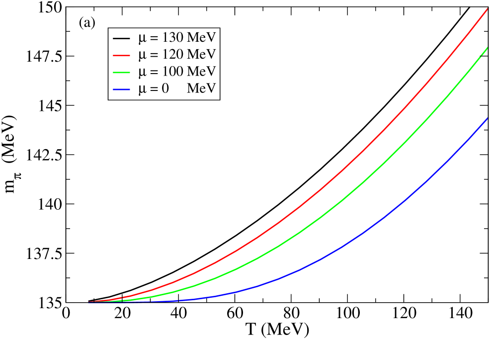
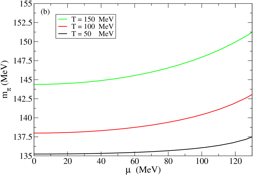
Figure 3: Thermal pion mass as a function of $(a)$ $T$ for different values of $\mu$ ranging from $\mu=0$ to $\mu=130$ MeV and as a function of $(b)$ $\mu$ for different values of $T$ ranging from $T=50$ to $T=150$ MeV.

Let us now pause briefly to describe the formalism that allows us to introduce a finite chemical potential associated to a conserved pion number. To this end, let us further modify the Lagrangian in Eq. (4), writing it in terms of a complex scalar field and regarding $\phi$ and $\phi^{*}$ as independent fields

$${\mathcal{L}}^{\prime}\rightarrow{\mathcal{L}}^{\prime\prime} = (D_{\mu}\phi)(D^{\mu}\phi^{*})-m_{\pi}^{2}\phi\phi^{*}-\frac{\alpha}{4}(\phi\phi^{*})^{2}$$ (5)

$$+ \frac{1}{2}m_{\rho}^{2}\rho^{\mu}\rho_{\mu}-\frac{1}{4}\rho_{\mu\nu}\rho^{\mu\nu}\,.$$

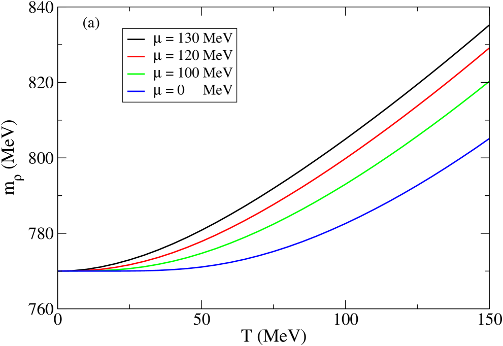
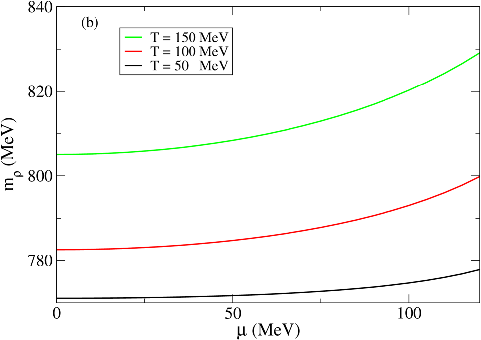
Figure 4: Thermal $\rho$ mass as a function of $(a)$ $T$ for different values of $\mu$ ranging from $\mu=0$ to $\mu=130$ MeV and as a function of $(b)$ $\mu$ for different values of $T$ ranging from $T=50$ to $T=150$ MeV.

The effective Lagrangian in Eq. (5) resembles that of scalar electrodynamics with the photon field replaced by the massive $\rho$ field. Invariance under global phase transformations

$$\phi\rightarrow\phi^{\prime}=e^{-i\lambda}\phi$$ (6)

leads to the conserved current

$$J^{\mu}=i(\phi^{*}\partial^{\mu}\phi-\phi\ \partial^{\mu}\phi^{*})-2g\rho^{\mu}\phi^{*}\phi\,,$$ (7)

and to the conserved charge $N$, that can be identified with the particle number, given by

$$N=i\int d^{3}x(\phi^{*}\partial^{0}\phi-\phi\ \partial^{0}\phi^{*}+2ig\rho^{0}\phi^{*}\phi)\,.$$ (8)

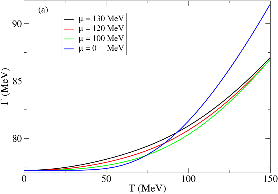
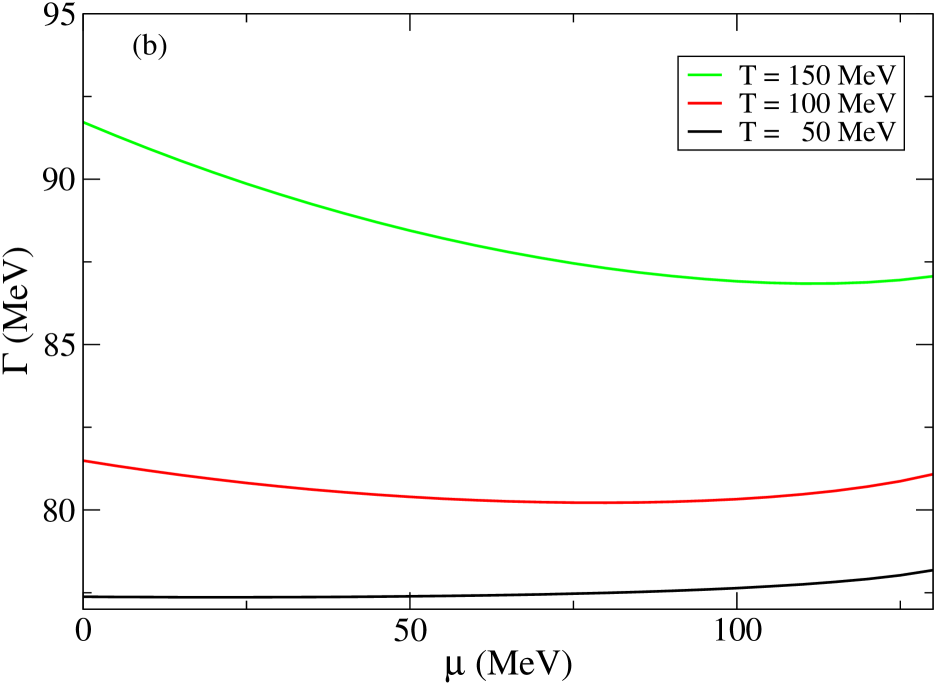
Figure 5: Thermal $\rho$ half width as a function of $(a)$ $T$ for different values of $\mu$ ranging from $\mu=0$ to $\mu=130$ MeV and as a function of $(b)$ $\mu$ for different values of $T$ ranging from $T=50$ to $T=150$ MeV.

Since $N$ is a conserved charge, there exists a chemical potential $\mu$ conjugate to $N$ so that the grand partition function is

$$Z(\beta,\mu)={\mbox{Tr}}\ e^{-\beta(H-\mu N)}\,,$$ (9)

where $\beta=1/T$ is the inverse of the temperature $T$. From now on, let us work explicitly in the imaginary-time formalism of thermal field theory. It is straightforward to write a path integral representation in Euclidean space of the grand partition function $Z(\beta,\mu)$. Care has to be taken by going through the Hamiltonian form since $N$ depends on the time derivative of $\phi$ and $\phi^{*}$. After integration over the conjugate fields $\pi^{*}=\partial{\mathcal{L}}^{\prime\prime}/\partial(\partial^{0}\phi^{*})$ and $\pi=\partial{\mathcal{L}}^{\prime\prime}/\partial(\partial^{0}\phi)$ one can check that in the exponent, there appear the combinations

$$-\phi^{*}\left(\frac{\partial^{2}}{\partial\tau^{2}}-2\mu\frac{\partial}{\partial\tau}+\mu^{2}-m_{\pi}^{2}\right)\phi\,,$$ (10)

$$ig\rho^{0}\left(\phi^{*}\frac{\partial\phi}{\partial\tau}-\phi\frac{\partial\phi^{*}}{\partial\tau}\right)-2ig\mu\rho^{0}\phi^{*}\phi\,,$$ (11)

where $\tau$ is the Euclidean time. Going to frequency space the Euclidean time derivatives get replaced by

$$\frac{\partial\phi}{\partial\tau} \rightarrow -i\omega_{n}\phi$$

$$\frac{\partial\phi^{*}}{\partial\tau} \rightarrow i{\omega}_{n^{\prime}}\phi^{*}\,,$$ (12)

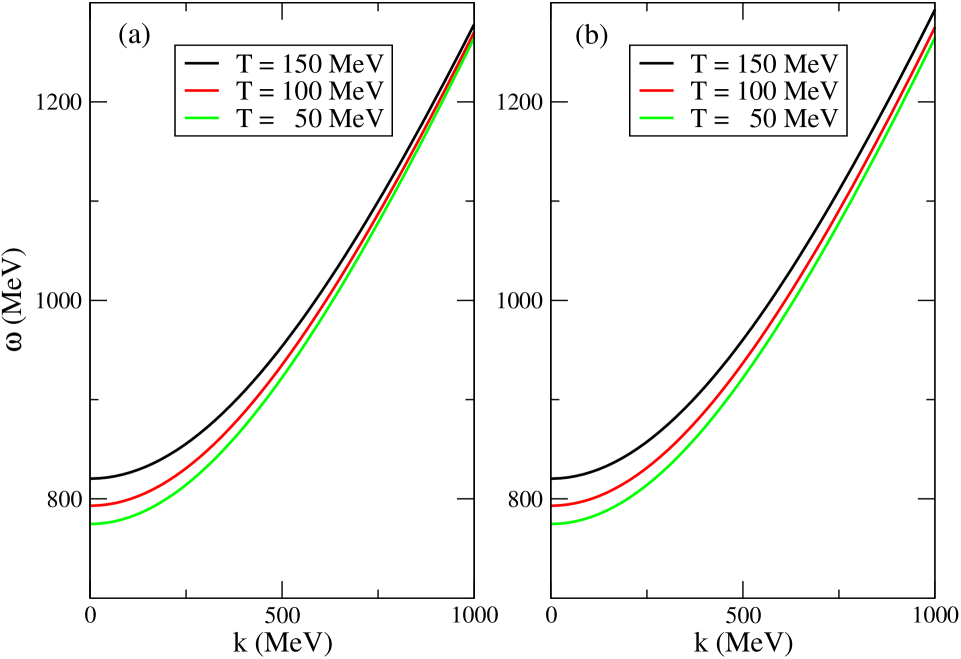
Figure 6: $\rho$ dispersion relation for $(a)$ longitudinal and $(b)$ transverse modes for $\mu=100$ MeV for different values of $T$ ranging from $T=50$ to $T=150$ MeV.

where the periodicity of the fields in the interval $0\leq\tau\leq\beta$ makes the (Matsubara) frequencies $\omega_{n}$ and ${\omega}_{n^{\prime}}$ be discrete and integer multiples of $2\pi T$. The combination in Eq. (10) translates into a modification of the Matsubara pion propagator which now reads as (hereafter capital letters are used to denote four-vectors whereas lower case letters are used do denote the components)

$$\Delta(i\omega_{n},p;\mu)=\frac{1}{-(i\omega_{n}+\mu)^{2}+p^{2}+m_{\pi}^{2}}\,,$$ (13)

whereas the combination in Eq. (11) goes into a modification of the $\pi$-$\rho$ vertex which now becomes

$$\Gamma_{\pi\rho}(P_{\mu},{P^{\prime}}_{\mu};\mu) = -ig\{[-(i\omega_{n}+\mu),{\mathbf{p}}]$$ (14)

$$+ [-(i{\omega}_{n^{\prime}}+\mu),{\mathbf{p}^{\prime}}]\}\,,$$

The final outcome is that the introduction of a finite chemical potential translates into the substitution

$$i\omega_{n}\rightarrow i\omega_{n}+\mu$$ (15)

both when this frequency appears in internal pion lines either in the Matsubara propagator or in the the $\pi$-$\rho$ vertex. Notice that these substitutions agree with the weel known result for the periodicity of the Matsubara propagator in the mixed representation given by

$$\Delta(\beta-\tau,E;\mu)=\Delta(\tau,E;-\mu)\,.$$ (16)

III $\pi$ self-energy

The effective Lagrangian in Eq. (5) describes the interactions between pions and $\rho$’s as well as among pions themselves. The one-loop diagrams for the pion and $\rho$ self-energies are depicted in Figs. 1 and 2. For the pion self-energy, the diagrams contain terms with internal $\rho$ propagators. Notice that since $m_{\rho}\gg m_{\pi},\ T$, these diagrams are strongly suppressed at finite temperature compared to those made out exclusively of internal pion lines and can thus be neglected. This approximation goes along the lines of the reasoning used in Refs. Ayala where the heavy internal sigma modes were systematically pinched to construct the effective vertices and propagators leading to the effective Lagrangian in Eq. (1). In this scheme, the pion and $\rho$ self-energies decouple and the former gets modified only by the diagram in Fig. 1a leading to a momentum independent correction of the pion mass. We can thus take one step further going beyond naive perturbation theory and adopt a resummation scheme for the pion self-energy to look for the modification of the pion mass beyond leading order. This can be implemented by writing the pion self-energy explicitly as

$$\Pi_{0}=\frac{\alpha}{2}T\sum_{n}\int\frac{d^{3}k}{(2\pi)^{3}}\frac{1}{K^{2}+m_{\pi}^{2}+\Pi_{0}}\,,$$ (17)

Equation (17) represents a self consistent relation for the temperature and density dependent quantity $\Pi_{0}$. This is the well known resummation for the superdaisy diagrams which constitute the dominant contribution in the large-$N$ expansion Dolan of the Lagrangian in Eq. (1). The solution to Eq. (17) is given by the transcendental equation

$$\Pi_{0} = \left(\frac{\alpha T}{4\pi^{2}}\right)\sqrt{m_{\pi}^{2}+\Pi_{0}}$$ (18)

$$\times \sum_{n=1}^{\infty}K_{1}\left(\frac{n\sqrt{m_{\pi}^{2}+\Pi_{0}}}{T}\right)\frac{\cosh(n\mu/T)}{n}\,.$$

Figure 3 shows the behavior of the pion thermal mass $\tilde{m}_{\pi}=\sqrt{m_{\pi}^{2}+\Pi_{0}}$ as a function of $(a)$ $T$ for different values of $\mu$ and $(b)$ as a function of $\mu$ for different values of $T$. We use the values $m_{\pi}=135$ MeV, $f_{\pi}=93$ MeV. From Fig. 3, we notice that $\tilde{m}_{\pi}$ grows monotonically with both $T$ and $\mu$.

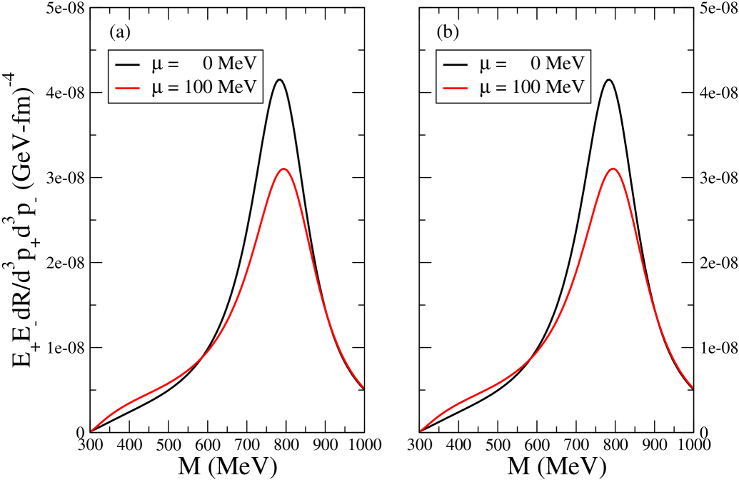
Figure 7: Dilepton production rates for $(a)$ longitudinal and $(b)$ transverse modes for $T=150$ MeV, $k=50$ MeV and $\mu=0,100$ MeV.

IV $\rho$ self-energy

The explicit expression for the one-loop $\rho$ self-energy depicted in Fig. 2 is given by

$$\Pi^{\mu\nu} = -g^{2}T\sum_{n}\int\frac{d^{3}p}{(2\pi)^{3}}\frac{(2P^{\mu}-K^{\mu})(2P^{\nu}-K^{\nu})}{(P^{2}+\tilde{m}_{\pi}^{2})[(K-P)^{2}+\tilde{m}_{\pi}^{2}]}$$ (19)

$$+ \delta^{\mu\nu}g^{2}T\sum_{n}\int\frac{d^{3}p}{(2\pi)^{3}}\frac{1}{P^{2}+\tilde{m}_{\pi}^{2}}\,,$$

where, according to the discussion in Sec. II, the internal pion momentum $P^{\mu}$ and the $\rho$ momentum $K^{\mu}$ are

$$P^{\mu} = [-(i\omega_{n}+\mu),{\mathbf{p}}]$$

$$K^{\mu} = (-i\omega,{\mathbf{k}})\,.$$ (20)

Equation (19) contains vacuum and matter contributions. It is well known that the infinities coming from the vacuum pieces can be reabsorbed into the redefinition of the bare masses and couplings Gale . For what follows, we will concentrate on the matter contributions.

Figure 8: Dilepton production rates for $(a)$ longitudinal and $(b)$ transverse modes for $T=150$ MeV, $k=250$ MeV and $\mu=0,100$ MeV.

For a massive vector field, the tensor structure of its self-energy can be written in terms of the longitudinal $P_{L}^{\mu\nu}$ and transverse $P_{T}^{\mu\nu}$ projection tensors

$$\Pi^{\mu\nu}=F(K)P_{L}^{\mu\nu}+G(K)P_{T}^{\mu\nu}\,.$$ (21)

In Minkowski space, $P_{T,L}^{\mu\nu}$ are given by

$$P_{T}^{00} = P_{T}^{0i}=P_{T}^{i0}=0$$

$$P_{T}^{ij} = \delta^{ij}-k^{i}k^{j}/k^{2}$$

$$P_{L}^{\mu\nu} = -g^{\mu\nu}+K^{\mu}K^{\nu}/K^{2}-P_{T}^{\mu\nu}\,.$$ (22)

From the relation between the self-energy, and the full $D^{\mu\nu}$ and bare $D^{\mu\nu}_{0}$ $\rho$ propagators, we have, also in Minkowski space

$$-iD^{\mu\nu}=\frac{P_{L}^{\mu\nu}}{K^{2}-m_{\rho}^{2}-F}+\frac{P_{T}^{\mu\nu}}{K^{2}-m_{\rho}^{2}-G}+\frac{K^{\mu}K^{\nu}}{m_{\rho}^{2}K^{2}}.$$ (23)

In order to identify the coefficients $F$ and $G$ of the longitudinal and transverse projectors, we take ${\mathbf{k}}$ along the $z$-axis. Thus, in Minkowski space, their expressions are

$$F(K) = -\frac{K^{2}}{k_{0}k}\Pi^{03}$$

$$G(K) = \Pi^{11}\,,$$ (24)

where $\Pi^{03}$ and $\Pi^{11}$ are obtained from Eq. (19) with the analytical continuation

$$i\omega\rightarrow k_{0}+i\epsilon\,,$$ (25)

that give the retarded functions and that can be performed after carrying out the sum over the Matsubara frequencies.

The sum over frequencies can be obtained by standard techniques Kapusta ; LeBellac . Considering the effects of a finite chemical potential, the expressions of interest are

$$T\sum_{n}\Delta(i\omega_{n},p)\Delta(i(\omega-\omega_{n}),|{\mathbf{k}}-{\mathbf{p}}|) = -\sum_{s_{1}s_{2}=\pm}\frac{s_{1}s_{2}}{4E_{p}E_{|{\mathbf{k}}-{\mathbf{p}}|}}\frac{[1+n(s_{1}E_{p}-\mu)+n(s_{2}E_{|{\mathbf{k}}-{\mathbf{p}}|}+\mu)]}{(i\omega-s_{1}E_{p}-s_{2}E_{|{\mathbf{k}}-{\mathbf{p}}|})}$$

$$T\sum_{n}i\omega_{n}\Delta(i\omega_{n},p)\Delta(i(\omega-\omega_{n}),|{\mathbf{k}}-{\mathbf{p}}|) = -\sum_{s_{1}s_{2}=\pm}\frac{s_{1}s_{2}(s_{1}E_{p}-\mu)}{4E_{p}E_{|{\mathbf{k}}-{\mathbf{p}}|}}\frac{[1+n(s_{1}E_{p}-\mu)+n(s_{2}E_{|{\mathbf{k}}-{\mathbf{p}}|}+\mu)]}{(i\omega-s_{1}E_{p}-s_{2}E_{|{\mathbf{k}}-{\mathbf{p}}|})}\,,$$ (26)

where

$$n(x)=\frac{1}{e^{\beta|x|}-1}\,,$$ (27)

is the Bose-Einstein distribution, $E_{p}=\sqrt{p^{2}+\tilde{m}_{\pi}^{2}}$, $E_{|{\mathbf{k}}-{\mathbf{p}}|}=\sqrt{({\mathbf{k}}-{\mathbf{p}})^{2}+\tilde{m}_{\pi}^{2}}$ and the function $\Delta$ is defined in Eq. (13).

Using Eq. (26) into Eq. (19) and by means of the analytical continuation in Eq. (25), the real and imaginary parts of $\Pi^{03}$ and $\Pi^{11}$ are given by

$${\mbox{Re}}\Pi^{03} = \frac{g^{2}}{8\pi^{2}}\int_{0}^{\infty}dp\left(\frac{p^{2}}{E_{p}}\right)\left[n(E_{p}-\mu)+n(E_{p}+\mu)\right]\left[k_{0}(A_{-}+A_{+})-2E_{p}(A_{-}-A_{+})\right]$$

$${\mbox{Im}}\Pi^{03} = \frac{g^{2}}{16\pi}\left(\frac{k_{0}}{k^{2}}\right)\Big{\{}\int_{\frac{k_{0}-ak}{2}}^{\frac{k_{0}+ak}{2}}dE_{p}(2E_{p}-k_{0})^{2}[1+2n(E_{p}-k_{0}-\mu)]\theta(k_{0})$$

$$- \int_{\frac{-k_{0}-ak}{2}}^{\frac{-k_{0}+ak}{2}}dE_{p}(2E_{p}+k_{0})^{2}[1+2n(E_{p}+k_{0}+\mu)]\theta(-k_{0})\Big{\}}$$

$${\mbox{Re}}\Pi^{11} = \frac{g^{2}}{8\pi^{2}}\int_{0}^{\infty}dp\left(\frac{p^{2}}{E_{p}}\right)\left[n(E_{p}-\mu)+n(E_{p}+\mu)\right]\left[\frac{2(k_{0}^{2}+k^{2})}{k^{2}}+(B_{-}+B_{+})\right]$$

$${\mbox{Im}}\Pi^{11} = -\frac{g^{2}}{32\pi}\left(\frac{1}{k^{3}}\right)\Big{\{}\int_{\frac{k_{0}-ak}{2}}^{\frac{k_{0}+ak}{2}}dE_{p}[4p^{2}k^{2}-(k^{2}-k_{0}^{2}+2k_{0}E_{p})^{2}][1+2n(E_{p}-k_{0}-\mu)]\theta(k_{0})$$

$$- \int_{\frac{-k_{0}-ak}{2}}^{\frac{-k_{0}+ak}{2}}dE_{p}[4p^{2}k^{2}-(k^{2}-k_{0}^{2}-2k_{0}E_{p})^{2}][1+2n(E_{p}+k_{0}+\mu)]\theta(-k_{0})\Big{\}}$$

$$A_{\pm} = \frac{1}{2k^{2}p}\left(4kp+[k_{0}^{2}\pm 2k_{0}E_{p}]\ln\left|\frac{k_{0}^{2}-k^{2}\pm 2k_{0}E_{p}-2kp}{k_{0}^{2}-k^{2}\pm 2k_{0}E_{p}+2kp}\right|\right)$$

$$B_{\pm} = \left(\frac{(k_{0}^{2}-k^{2}\pm 2k_{0}E_{p})^{2}-4k^{2}p^{2}}{4k^{3}p}\right)\ln\left|\frac{k_{0}^{2}-k^{2}\pm 2k_{0}E_{p}-2kp}{k_{0}^{2}-k^{2}\pm 2k_{0}E_{p}+2kp}\right|\,,$$ (28)

where the function $a$ is defined as

$$a=\sqrt{1-\frac{4\tilde{m}_{\pi}^{2}}{(k_{0}^{2}-k^{2})}}\,.$$ (29)

It is easy to check that in the limit $\mu\rightarrow 0$, Eqs. (28) reduce to the corresponding expressions found in Ref. Gale .

Figure 4 shows the behavior of the $\rho$ thermal mass obtained as the solution for $k_{0}$ of either

$$k_{0}^{2}-m_{\rho}^{2}-{\mbox{Re}}\left\{\begin{array}[]{c}F(k_{0},k=0)\\ G(k_{0},k=0)\end{array}\right\}=0\,,$$ (32)

as a function of $(a)$ $T$ for different values of $\mu$ and $(b)$ as a function of $\mu$ for different values of $T$. We use the value $g^{2}/4\pi=2.93$ as determined by the $\rho$ width in vacuum. For $k=0$ there is no distinction between transverse and longitudinal modes and thus both Eqs. (32) lead to the same solution. For every value of $(T,\mu)$, the solution is computed with the corresponding value for $\tilde{m}_{\pi}(T,\mu)$. From Fig. 4, we see that the thermal $\rho$ mass grows monotonically with both $T$ and $\mu$ and that the growth is larger for larger values of $\mu$.

Figure 5 shows the behavior of the $\rho$ decay rate (or half width) obtained from either

$$\Gamma=-\frac{{\mbox{Im}}\left\{\begin{array}[]{c}F(m_{\rho}(T,\mu),k=0)\\ G(m_{\rho}(T,\mu),k=0)\end{array}\right\}}{2m_{\rho}(T,\mu)}$$ (35)

as a function of $(a)$ $T$ for different values of $\mu$ and $(b)$ as a function of $\mu$ for different values of $T$. Again, for $k=0$ there is no distinction between transverse and longitudinal modes. This can be shown analytically from the explicit expressions of ${\mbox{Im}}F$ and ${\mbox{Im}}G$ in Eqs. (28) which for $k=0$ yield

$${\mbox{Im}}F(k_{0},k=0) = {\mbox{Im}}G(k_{0},k=0)$$ (36)

$$= -\left(\frac{g^{2}}{48\pi}\right)k_{0}^{2}\left(1-\frac{4\tilde{m}_{\pi}^{2}}{k_{0}^{2}}\right)^{3/2}$$

$$\times \left[1+2n(k_{0}/2+\mu)\right]\,.$$

For $\mu=0$, Eq. (36) coincides with the corresponding expression in Ref. Gale .

From Fig. 5a we see that for a given value of $\mu$ the $\rho$ width increases monotonically with temperature. From Fig. 5b we observe that the width reaches a minimum at a finite value of $\mu$ and that this value increases as the temperature increases. This behavior can be understood if we recall that when the density increases so does the pion mass and thus the phase space available for the decay products of $\rho$ narrows. The situation changes when the density is large enough so that the increase in the mass of the $\rho$ becomes steeper than the growth in the pion mass, widening the phase space available for the decay process.

Figure 6 shows the dispersion relation for $(a)$ longitudinal and $(b)$ transverse $\rho$ modes for different values of $T$ and $\mu=100$ MeV. The main difference between the curves in each set can be attributed to the increase of the $\rho$ mass with both $\mu$ and $T$.

V Dilepton rate

The electromagnetic current can be identified with the underlying quark structure of hadrons. For invariant masses below the charm threshold, this current can be decomposed as

$$j_{\mu}^{\ \mbox{\small{em}}}=\frac{2}{3}\bar{u}\gamma_{\mu}u-\frac{1}{3}\bar{d}\gamma_{\mu}d-\frac{1}{3}\bar{s}\gamma_{\mu}s\,.$$ (37)

Using the $SU(3)$ quark content of hadrons, this current, being vectorial in nature, can be in turn identified with the current constructed out of the vector mesons $\rho$, $\omega$ and $\phi$.

$$j_{\mu}^{\ \mbox{\small{em}}}=j_{\mu}^{\rho}+j_{\mu}^{\omega}+j_{\mu}^{\phi}\,,$$ (38)

This is the well known conjecture named vector dominance model (VDM). Since the pion electromagnetic form factor is is almost totally dominated by the $\rho$ for invariant masses below 1 GeV, a simplified picture to study the decay of this electromagnetic current into low mass dilepton pairs is to consider that the current in Eq. (38) is totally dominated by the $\rho$. A further simplification stems from considering the spectral density of $\rho$ as a simple pole located at its peak which in turn dictates that the coupling of $\rho$ to the electromagnetic current is $em_{\rho}^{2}/g$.

Under the assumption of VDM and $\rho$ saturation, the expressions for the thermal dilepton rates from longitudinal and transverse $\rho$ modes are given, respectively, by Gale

$$E_{+}E_{-}\frac{dR}{d^{3}p_{+}d^{3}p_{-}} = \frac{1}{(2\pi)^{6}}\left(\frac{e^{4}}{g^{2}}\right)\left(\frac{m_{\rho}^{4}}{M^{4}}\right)\left[q^{2}-\frac{({\mathbf{q}}\cdot{\mathbf{k}})^{2}}{k^{2}}\right]\frac{-{\mbox{Im}}F}{(M^{2}-m_{\rho}^{2}-{\mbox{Re}}F)^{2}+{\mbox{Im}}F^{2}}\left(\frac{1}{e^{\beta\omega_{L}}-1}\right),$$

$$E_{+}E_{-}\frac{dR}{d^{3}p_{+}d^{3}p_{-}} = \frac{1}{(2\pi)^{6}}\left(\frac{e^{4}}{g^{2}}\right)\left(\frac{m_{\rho}^{4}}{M^{4}}\right)\left[2M^{2}-q^{2}+\frac{({\mathbf{q}}\cdot{\mathbf{k}})^{2}}{k^{2}}\right]\frac{-{\mbox{Im}}G}{(M^{2}-m_{\rho}^{2}-{\mbox{Re}}G)^{2}+{\mbox{Im}}G^{2}}\left(\frac{1}{e^{\beta\omega_{T}}-1}\right),$$ (39)

where $P^{\mu}_{+}=(E_{+},{\mathbf{p}}_{+})$ and $P^{\mu}_{-}=(E_{-},{\mathbf{p}}_{-})$ are the positron and electron four momenta, respectively, $K^{\mu}=P^{\mu}_{+}+P^{\mu}_{-}$, $Q^{\mu}=P^{\mu}_{+}-P^{\mu}_{-}$, $M^{2}=k_{0}^{2}-k^{2}$ is the pair invariant mass, $\omega_{L,T}$ are the longitudinal and transverse $\rho$ modes dispersion relations and we have neglected the electron mass.

Figures 7 and 8 show the dilepton production rates as functions of the pair invariant mass $M$ for ${\mathbf{q}}\cdot{\mathbf{k}}=0$ for fixed values of $T=150$ MeV and $k$ for two values of $\mu=0,100$ MeV for $(a)$ longitudinal and $(b)$ transverse modes. Figure 7 considers an small value of $k=50$ MeV and Fig. 8 a larger value $k=250$ MeV. In both cases we can see that the effect of the finite chemical potential is to moderately widen the distribution and to (also moderately) displace the position of the peak toward larger values of $M$. The most significant effect is however the lowering of the peak for finite $\mu$ which is in agreement with the analysis of Ref. Rapp2 .

VI Summary and conclusions

In this paper we have considered the effects of a finite pion density on the propagation properties of $\rho$ mesons at finite temperature. The $\rho$ has been introduced by gauging an effective Lagrangian obtained from the linear sigma model in the kinematical regime where the pion mass and temperature are small compared to the sigma mass. The finite density is described in terms of a finite pion chemical potential associated to a conserved pion number. We have argued that such description is important for ultra relativistic heavy-ion collisions at RHIC and LCH energies where the central rapidity region is expected to become baryon free. In this situations, we expect that the influence of the dropping $\rho$ mass or melting or resonances scenarios to describe the dilepton spectra, which rely on the effects of a finite baryon density, become less important than the effects of the expected large pion density. This is so particularly during the hadronic phase of the reaction, between chemical and thermal freeze-out when the strong interaction drives pion-number to a fixed value.

We have found that the $\rho$ thermal mass increases monotonically with both the temperature and the pion density. However, the $\rho$ width as a function of $\mu$ and for fixed $T$ starts off by decreasing, reaching a minimum at a finite value of $\mu$. This behavior can be understood by noticing that as the density increases, the pion mass does too and the phase space available for the decay process $\rho\rightarrow\pi\pi$ narrows up to a –temperature dependent– value of $\mu$. From this value, the increase in the thermal $\rho$ mass is stronger than the increase in the thermal pion mass and this effect produces a widening of the phase space for the process, thus producing the $\rho$ width to rise.

Under the assumption of VDM and $\rho$ saturation, we have also computed the dilepton production rate as a function of the pair invariant mass. We have found that the finite pion density produces a moderate broadening of the distribution and a moderate increase of the position of the peak. The finite pion density also produces a decrease of the distribution at the position of the peak compared to the $\mu=0$ case.

The problem posed by the renormalization of theories involving resummation is by no means a simple one. In fact, in recent years this subject has been much actively pursued in the literature (see for example Refs. Hees ; Caldas ; Blaizot ). The consensus is that when the theory is vacuum renormalizable, it will still be renormalizable after resummation. The solution, which can be formulated using different languages, has been shown to require that the counterterms needed for vacuum renormalization in ordinary perturbation theory need also to receive the benefits of resummation and be considered self-consistently in the resummation procedure.

For the purposes of our work, let us stress that the resummation we have implemented for the pion self-energy corresponds to the tadpole approximation (see Sec III of Ref. Hees ). In fact, the gap equation that renders the finite temperature and density corrections to the pion mass in our work, Eq. (18), is identical to the thermal part of Eq. (24) of the above reference; we have just gone one step further, expanding the integrand as a series which allows us to analytically integrate each term. In Eq. (24) of Ref. Hees , the renormalization of the vacuum self energy and four-point function have been carried out on the physical mass-shell condition and have taken into account the self-consistency. In the language of this reference, this is so because in the tadpole approximation, the renormalized four-point function is constant and given just in terms of the original coupling constant on the mass-shell condition.

Had we gone beyond the tadpole approximation, the situation would have not be that straightforward. In fact, it has also been shown in Ref. Hees that the self-consistent resummation scheme requires a more complicated renormalization of the four-point function to be taken into account alongside the renormalization procedure for the self-energy. The effects of this certainly more complete analysis might be interesting with regard to further thermal modifications to the pion mass in situations where the original coupling constant of the $\phi^{4}$ theory is much larger that one but is certainly beyond the scope of the present work where our coupling constant $\alpha$, as determined by the scale of the interactions, set by the vacuum pion mass, is of order 1 (in fact, what matters, as shown in Eq. (18) is the effective coupling constant given by $\alpha/(4\pi^{2})$ which is of order 0.1).

Finally, in order to predict the final dilepton spectra at RHIC and LHC energies, the results found in this work have to be placed into a model for the evolution of the collision and also possibly to include the effects of other vector or axial vector mesons. All this is for future.

References

- (1) G. Roche et al., (DLS Collaboration) Phys. Lett. B226, 228 (1989); S. Bedoe et al., (DLS Collaboration) Phys. Rev. C47, 2840 (1993); G. Agakichiev et al., (CERES Collaboration), Phys. Rev. Lett. 75, 1272 (1995); D. Adamová et al., (CERES/NA45 Collaboration), Enhanced production of low mass electron pairs in 40 AGeV Pb-Au collisions at the CERN-SPS, nucl-ex/0209024.
- (2) For a comprehensive review of the theoretical and experimental status on the subject see R. Rapp and J. Wambach, Adv. Nucl. Phys. 25, 1 (2000).
- (3) G.E. Brown and M. Rho, Phys. Rev. Lett. 66, 2720 (1991).
- (4) C. Dominguez and M. Loewe, Z. Phys. C 49, 423 (1991).
- (5) M. Asakawa, C.M. Ko, P. Lévai and X.J. Qiu, Phys. Rev. C46, R1159 (1992).
- (6) J. Chen, J. Li and P. Zhuang, JHEP, 0211, 14 (2002).
- (7) H. Bebie, P. Gerber, J.L. Goity and H. Leutwyler, Nucl. Phys. B378, 95 (1992).
- (8) P. Braun-Munzinger, J. Stachel, J. Wessels, and N. Xu, Phys. Lett. B344, 43 (1995), ibid 365, 1 (1996).
- (9) C.M. Hung and E. Shuryak, Phys. Rev. C 57, 1891 (1998).
- (10) C. Song and V. Koch, Phys. Rev. C 55, 3026 (1997).
- (11) D. Teaney, Chemical freezeout in heavy ion collisions, nucl-th/0204023 (2002); T.Hirano and K. Tsuda, Phys. Rev. C66, 054905 (2002).
- (12) M. Loewe and C. Villavicencio, Thermal pions at finite density, hep-ph/0206294, (2002); Thermal pions at finite isospin chemical potential, hep-ph/0212275.
- (13) A. Ayala, S. Sahu and M. Napsuciale, Phys. Lett. B 479, 156 (2000); A. Ayala and S. Sahu, Phys. Rev. D 62, 056007 (2000).
- (14) A. Ayala, P. Amore and A. Aranda, Phys. Rev. C66, 045205 (2002).
- (15) J. Gasser and H. Leutwyler, Phys. Lett. B184, 83 (1987).
- (16) C. Gale and J. Kapusta, Nucl. Phys. B357, 65 (1991).
- (17) R.D. Pisarski, Phys. Rev. D52, R3773 (1995).
- (18) L. Dolan and R. Jackiw, Phys. Rev. D 9, 3320 (1974); S. Weinberg, ibid 9, 3357 (1974).
- (19) J.I. Kapusta, Finite Temperature Field Theory (Cambridge University Press, Cambridge, 1989).
- (20) M. Le Bellac, Thermal Field Theory (Cambridge University Press, Cambridge, 1996).
- (21) R. Rapp and C. Gale, Phys. Rev. C60, 024903 (1999).
- (22) H. van Hees and J. Knoll, Phys. Rev. D65, 105005 (2002).
- (23) H.C.G. Caldas, Phys. Rev. D65, 065005 (2002).
- (24) J.-P. Blaizot, E. Iancu and U. Reinosa, Renormalizability of derivable approximations in scalar theory, hep-ph/0301201.