[

WMAP and Inflation

Abstract

We assay how inflationary models whose properties are dominated by the dynamics of a single scalar field are constrained by cosmic microwave background (CMB) data from the Wilkinson Microwave Anisotropy Probe (WMAP). We classify inflationary models in a plane defined by the horizon-flow parameters. Our approach differs from that of the WMAP collaboration in that we analyze only WMAP data and take the spectral shapes from slow-roll inflation rather than power-law parameterizations of the spectra. The only other information we use is the measurement of $h$ from the Hubble Space Telescope (HST) Key Project. We find that the spectral index of primordial density perturbations lies in the $1\sigma$ range $0.94\leq n_{s}\leq 1.04$ with no evidence of running. The ratio of the amplitudes of tensor and scalar perturbations is smaller than $0.61$ and the inflationary scale is below 2.8$\times 10^{16}$ GeV, both at the 2$\sigma$ C. L. No class of inflation or ekpyrotic/cyclic model is excluded. The $\lambda\phi^{4}$ potential is excluded at $3\sigma$ only if the number of e-folds is assumed to be less than 45.

]

That there are multiple peaks in the CMB has recently been reinforced by data from the WMAP satellite [1, 2, 3]. This establishes that the curvature fluctuations which seed structure formation were generated at superhorizon scales. The inflationary paradigm [4], which hinges on this very fact [5], is therefore vindicated. Other generic predictions of inflation, including approximate scale-invariance of the power spectra, flatness of the Universe and adiabaticity and gaussianity of the density perturbations are also fully consistent with WMAP data [6].

Given this supporting evidence for inflation, we adopt the full set of predictions of slow-roll inflation and obtain constraints on inflationary models imposed by WMAP’s data. Studies of this type have been carried out in the past with less precise data [7] and with the simple parameterization of the power spectra as power laws [8]. It has been emphasized that to extract precise information from data of WMAP’s quality, high-accuracy predictions of the power spectra resulting from slow-roll inflation should be used [9]. There is a wealth of cosmological information in the CMB [10], and our approach is to employ precise theoretical expectations in its extraction.

Since the WMAP collaboration has considered what implications their data have for inflation [11], we describe at the outset the differing elements between our analysis and theirs. We elaborate on these differences later. WMAP include CBI [12], ACBAR [13], 2dFGRS [14] and Lyman-$\alpha$ power spectrum [15] data in addition to their own data. We restrict ourselves to WMAP data with a top-hat prior on the Hubble constant $h$ ($H_{0}=100h$ km/s/Mpc), from the HST [16]. While we use the actual theoretical predictions for the primordial power spectra from single-field slow-roll inflation, WMAP parameterize the spectra with power-laws and a running spectral index. As a result, the spectral shapes we use are different from those of WMAP and we directly fit to slow-roll parameters, while WMAP fit to derivative quantities. There are different virtues of the two approaches, and a comparison of the results obtained from them serve as a check of the robustness of the conclusions reached.

Primordial spectra:

The primordial scalar and tensor power spectra to ${\cal O}(\ln^{2}k)$ are [9, 17]

$$P_{\chi} = A_{s}\big{(}a_{0}+a_{1}\ln{k\over k_{\star}}+a_{2}\ln^{2}{k\over k_{\star}}\big{)}\,,$$ (1)

$$P_{h} = A_{t}\big{(}b_{0}+b_{1}\ln{k\over k_{\star}}+b_{2}\ln^{2}{k\over k_{\star}}\big{)}\,,$$ (2)

where the pivot $k_{\star}$ typifies scales probed by the CMB. The constants $a_{i}$ and $b_{i}$ are functions [9, 18] of the horizon-flow parameters, $\epsilon_{i}$ of Ref. [19], that are defined by

$$\epsilon_{i+1} = {d\ln|\epsilon_{i}|\over dN}\,,\ \ \ i\geq 0$$ (3)

$$\epsilon_{0} = {H_{I}\over H}\,.$$ (4)

Here, $N$ is the number of e-folds since some moment $t_{I}$ during inflation, when the Hubble parameter was $H_{I}$.

Note that to ${\cal O}(\epsilon^{2})$, the $b_{i}$ depend only on $\epsilon_{1}$ and $\epsilon_{2}$, while the $a_{i}$ depend on $\epsilon_{1}$, $\epsilon_{2}$ and $\epsilon_{3}$. We initially set $\epsilon_{3}=0$, but we then later demonstrate that the fit to the WMAP data is essentially not improved by including nonzero $\epsilon_{3}$. The reason for not simply using the $\epsilon_{3}$-independent ${\cal O}(\epsilon)$ expressions is that the ${\cal O}(\epsilon^{2})$ expressions are more accurate far from the pivot, and for a wider range of $\epsilon_{1}$ and $\epsilon_{2}$ [7, 9]. It is uncertain that even high-precision data from the Planck satellite [20] can constrain $\epsilon_{3}$ to be small. Including $\epsilon_{3}$ in our analysis would simply enlarge the allowed parameter space to include models which are not inflationary in the sense that the horizon-flow parameters are not small.

The primary advantage of the horizon-flow parameters is that accurate predictions of the shapes and normalizations of the power spectra can be made independent of parameters describing cosmic evolution. The horizon-flow parameters $\epsilon_{1}$ and $\epsilon_{2}$ are related to the usual slow-roll parameters [21]

$$\epsilon \equiv {M_{Pl}^{2}\over 16\pi}\big{(}{V^{\prime}\over V}\big{)}^{2}\,,$$ (5)

$$\eta \equiv {M_{Pl}^{2}\over 8\pi}\bigg{[}{V^{\prime\prime}\over V}-{1\over 2}\big{(}{V^{\prime}\over V}\big{)}^{2}\bigg{]}\,,$$ (6)

via the first order relations [9]

$$\epsilon_{1}\simeq\epsilon\,,\ \ \ \ \ \ \ \epsilon_{2}\simeq 2(\epsilon-\eta)\,.$$ (7)

The normalizations of the spectra are given by

$$A_{s}={H_{I}^{2}\over\pi\epsilon_{1}M_{Pl}^{2}}\,,\ \ \ \ \ \ \ A_{t}={16H_{I}^{2}\over\pi M_{Pl}^{2}}\,,$$ (8)

and the ratio of the amplitudes of the spectra at the pivot $k=k_{\star}$, is

$$R \equiv {A_{t}b_{0}\over A_{s}a_{0}}=16\epsilon_{1}\big{[}1+C\epsilon_{2}$$ (10)

$$+\big{(}C-{\pi^{2}\over 2}+5\big{)}\epsilon_{1}\epsilon_{2}+\big{(}{C^{2}\over 2}-{\pi^{2}\over 8}+1\big{)}\epsilon_{2}^{2}\big{]}\,,$$

where $C\equiv\gamma_{E}+\ln 2-2\approx-0.7296$. Note that $a_{0}$ and $b_{0}$ are ${\cal O}(1)$ and $|a_{0}-b_{0}|$ is ${\cal O}(\epsilon_{2})$. The spectral indices and their running can be expressed in terms of $\epsilon_{1}$, $\epsilon_{2}$ and $\epsilon_{3}$:

$$n_{s} = 1-2\epsilon_{1}-\epsilon_{2}-2\epsilon_{1}^{2}-(2C+3)\epsilon_{1}\epsilon_{2}-C\epsilon_{2}\epsilon_{3}\,,$$ (11)

$$n_{t} = -2\epsilon_{1}-2\epsilon_{1}^{2}-2(C+1)\epsilon_{1}\epsilon_{2}\,,$$ (12)

$$\alpha_{s} \equiv {dn_{s}\over d\ln k}=-2\epsilon_{1}\epsilon_{2}-\epsilon_{2}\epsilon_{3}\,,$$ (13)

$$\alpha_{t} \equiv {dn_{t}\over d\ln k}=-2\epsilon_{1}\epsilon_{2}\,.$$ (14)

We set $\epsilon_{i}=0$, $i\geq 3$. $R$, $n_{s}$ are $n_{t}$ are interdependent and the following consistency condition on single-field slow-roll inflation applies:

$$R\simeq-8n_{t}$$ (15)

By our choice of formalism, we implicitly assume this condition to be satisfied.

Note that the six inflationary parameters, $A_{s}$, $A_{t}$, $n_{s}$, $n_{t}$, $\alpha_{s}$ and $\alpha_{t}$ are determined by just three parameters, $A_{s}$, $\epsilon_{1}$ and $\epsilon_{2}$ in our analysis. In contrast, the WMAP collaboration parameterize the power-spectra with [11]

$$P_{\chi}=A_{s}\big{(}{k\over k_{\star}}\big{)}^{n_{s}-1+{1\over 2}\alpha_{s}\ln{k\over k_{\star}}}\,,\ \ \ \ P_{h}=A_{t}\big{(}{k\over k_{\star}}\big{)}^{n_{t}}\,.$$ (16)

They eliminate $n_{t}$ as a free parameter by using the consistency condition Eq. (15). Thus, they have four free parameters, $A_{s}$, $A_{t}$, $n_{s}$ and $\alpha_{s}$ and set $\alpha_{t}=0$.

A convenient classification of models based on the separate regions in the $R-n_{s}$ plane they populate, or equivalently relationships between the slow-roll parameters, was introduced in Ref. [22]. This classification becomes particularly simple in the $\epsilon_{2}-\epsilon_{1}$ plane, as discussed in the following section and shown in Fig. 3.

Inflation models:

In what follows we use the common jargon, “red-tilt” for $n_{s}<1$ and “blue-tilt” for $n_{s}>1$.

a) Canonical potentials of large-field models are the monomial potential,

$$V(\phi)=V_{0}(\phi/\mu)^{p}\,,\ \ \ \ p\geq 2\,,$$ (17)

and the exponential potential $V(\phi)=V_{0}e^{\phi/\mu}$ of power-law inflation. They are typical of chaotic inflation [23] and have $V^{\prime\prime}>0$. The value of the scalar field falls ${\cal O}(M_{Pl})$ while the relevant perturbations are generated and thereby offer a glimpse into Planckian physics. In terms of the horizon-flow parameters, large-field models satisfy

$$0\leq\epsilon_{2}<4\epsilon_{1}\,.$$ (18)

They have large $R$ and predict a red tilt.

b) Generic small-field potentials are of the form

$$V(\phi)=V_{0}[1-(\phi/\mu)^{p}]\,,\ \ \ \ p\geq 2\,,$$ (19)

and are therefore characterized by $V^{\prime\prime}<0$. The scalar field rolls from an unstable equilibrium at the origin towards a non-zero vacuum expectation value. Models relying on spontaneous symmetry breaking yield such potentials [24]. For small-field models

$$\epsilon_{2}>4\epsilon_{1}\,.$$ (20)

The tensor fraction is small and the scalar spectrum is red-tilted.

c) Potentials for hybrid inflation [25] are of the form

$$V(\phi)=V_{0}[1+(\phi/\mu)^{p}]\,,\ \ \ \ p\geq 2\,.$$ (21)

Hybrid inflation models involve multiple scalar fields. One of the fields, $\phi$, is the slowly rolling inflaton which does not carry most of the energy density ($\phi<\mu$). Another field which has a fixed value during the slow-roll of $\phi$ provides $V_{0}$. When $\phi$ falls below a critical value, the other field is destabilized and promptly ends inflation. As a result the value of $\phi$ at the end of inflation is very model-dependent, which makes the number of e-folds correspondingly uncertain. Hybrid models can be treated as single-field models because the only role of the second field is to end inflation, and the slow-roll dynamics is dominated by a single field. These potentials arise in supersymmetric and supergravity models of inflation. Hybrid models have

$$\epsilon_{2}<0\,.$$ (22)

There is no robust prediction for $R$ as can be seen from the above $\epsilon_{1}$-independent inequality. However, a unique prediction of these models is that the spectrum is blue-tilted if $|\epsilon_{2}|>2\epsilon_{1}$.

The line $\epsilon_{2}=0$ ($R=8(1-n_{s})$) implies $\epsilon=\eta$ which occurs for the exponential potential. Thus, power-law inflation marks the boundary between large-field and hybrid models.

c) Linear potentials,

$$V(\phi)=V_{0}(\phi/\mu)\,,\ \ \ \ V(\phi)=V_{0}[1-(\phi/\mu)]\,,$$ (23)

define the boundary between large and small field models and lie at

$$\epsilon_{2}=4\epsilon_{1}\,\ \ \ {\rm{or}}\ \ \ 3R=8(1-n_{s})\,.$$ (24)

Since $\epsilon_{1}$ is a constant for such potentials, inflation ends only with the help of an auxiliary field or some other physics.

To avoid overstating the comprehensiveness of this classification of potentials, we list a few potentials of different forms [26], which however do fit into the large-field, small-field, hybrid or linear categories according to the relationships between the horizon-flow parameters. $V(\phi)=V_{0}[1\pm\ln(\phi/\mu)]$, $V_{0}[1-e^{-\phi/\mu}]$ and $V_{0}[1\pm(\phi/\mu)^{-p}]$ are hybrid in the sense that an auxiliary field is needed to end inflation, but lead to $\epsilon_{2}>4\epsilon_{1}$ and therefore lie in the small-field region of the parameter space. Similarly, power-law inflation does not end without a hybrid mechanism, but lies in the large-field region. Finally, let us note that the simplest models of the ekpyrotic/cyclic [27] variety are small-field [28]; however, the prediction for $n_{s}$ in these models is controversial [29].

Analysis:

We compute the TT and TE power spectra $\delta T_{l}^{2}=l(l+1)C_{l}/2\pi$, using the Code for Anisotropies in the Microwave Background or CAMB [30] (which is a parallelized version of CMBFAST [31]) and a supporting module that calculates the inflationary predictions for the primordial scalar and tensor power spectra [32]. We assume the Universe to be flat, in accord with the predictions of inflation, and that the neutrino contribution to the matter budget is negligible. The dark energy is assumed to be a cosmological constant $\Lambda$. We calculate the angular power spectrum on a grid consisting of the parameters specifying the primordial spectra, $\epsilon_{1}$, $\epsilon_{2}$ and $A_{s}$, and those specifying cosmic evolution, the Hubble constant $h$, the reionization optical depth $\tau$, the baryon density $\omega_{b}=\Omega_{B}h^{2}$ and the total matter density $\omega_{M}=\Omega_{M}h^{2}$ (which is comprised of baryons and cold dark matter). We choose $h$ rather than $\Omega_{\Lambda}$ because it is directly constrained by the HST [16]. We do not include priors from supernova [33], gravitational lensing [34] or large scale structure [35] data or nucleosynthesis constraints on $\omega_{b}$ [36] although these would somewhat sharpen the cosmological parameter determinations.

We employ the following top-hat grid:

• $0.0001\leq\epsilon_{1}\leq 0.048$ in steps of size 0.004

• $-0.18\leq\epsilon_{2}\leq 0.14$ in steps of size 0.02

• $0.64\leq h\leq 0.80$ in steps of size 0.02

• $\tau=$0, 0.05, 0.1, 0.125, 0.15, 0.16, 0.17, 0.18, 0.19, 0.2, 0.25, 0.3

• $0.018\leq\omega_{b}\leq 0.028$ in steps of size 0.001

• $0.06\leq\omega_{M}\leq 0.22$ in steps of size 0.02

• $A_{s}$ is a continuous parameter.

The range of values chosen for $h$ correspond to the HST measurement, $h=0.72\pm 0.08$ [16]. This serves to break the degeneracy between $\Omega_{M}$ and $\Omega_{\Lambda}$ without the need for supernova data [37]. We place the pivot at $k_{\star}=0.007$ Mpc^-1. The primordial spectra are evaluated to ${\cal O}(\ln^{2}k)$ (see Eqs. 1-2) with $\epsilon_{3}=0$.

The WMAP data are in the form of 899 measurements of the TT power spectrum from $l=2$ to $l=900$ [2] and 449 data points of the TE power spectrum [3]. We compute the likelihood of each model of our grid using Version 1.1 of the code provided by the collaboration [38]. The WMAP code computes the full covariance matrix under the assumption that the off-diagonal terms are subdominant. This approximation breaks down for unrealistically small amplitudes. We include the off-diagonal terms only when the first peak occurs between $l=100$ and $l=400$ with a height above 5000 $\mu K^{2}$ [38]. The restriction on the peak location may at first appear irrelevant, but for very large tensor amplitudes, the maximum height of the scalar spectrum shifts to very small $l$. When the height of the first peak is below 5000 $\mu K^{2}$ (which is many standard deviations away from the data), we only use the diagonal terms of the covariance matrix to compute the likelihood. To obtain single-parameter constraints, we plot the relative likelihood $e^{(\chi^{2}_{min}-\chi^{2})/2}$, for each parameter after maximizing over all the others. The $x$-$\sigma$ range is obtained for likelihoods above $e^{-x^{2}/2}$. For 2-dimensional constraints, the $1\sigma$, $2\sigma$ and $3\sigma$ regions are defined by $\Delta\chi^{2}=2.3$, 6.17 and 11.83, respectively, for two degrees of freedom.

Results:

Although our primary focus is to obtain constraints on the inflationary models, we display constraints on the cosmological parameters as a consistency check with the WMAP collaboration. This is pertinent because we have used a form for the primordial spectra (Eqs. 1-2) that is specific to single-field slow-roll inflation rather than the standard power-law form.

The best-fit parameters are $\epsilon_{1}=0.016$, $\epsilon_{2}=-0.02$, $\omega_{b}=0.023$, $\omega_{M}=0.12$, $\tau=0.125$ and $h=0.78$ with normalization $A_{s}=22.0\times 10^{-10}$ with $\chi^{2}=1428.88$ for 1341 degrees of freedom. The results from Fig. 1 are in good agreement with those obtained by the WMAP collaboration [6]. This indicates that the choice of the spectral shapes does not matter at the present precision of the WMAP data.

FIG. 1.: Relative likelihood plots for several cosmological parameters and $A_{s}$. $t_{0}$ is the age of the Universe in Gyr. We do not show the plot for $h$ because it is not constrained by the fit; see Table. I.

FIG. 2.: Relative likelihood plots for some inflationary parameters.

Likelihood plots for the inflationary parameters are shown in Fig. 2. We do not show the result for $n_{t}$ because we have imposed the consistency condition, Eq. (15). The $1\sigma$ confidence limits on various parameters are provided in Table. I. We see that the spectra are consistent with scale-invariance and with a small tensor contribution; the best-fit scale-invariant spectrum with no tensor contribution has $\chi^{2}=1430.61$. Also, running of the spectral indices is insignificant. (In our framework $\alpha_{s,t}$ are required to be consistent with inflationary predictions as dictated by Eqs. (13) and (14); they are not free parameters).

$$\begin{array}[]{c|c|c|c}&1\sigma\ \rm{lower\ limit}&1\sigma\ \rm{upper\ limit}\\ \hline\cr\epsilon_{1}&0&0.028\\ \epsilon_{2}&-0.08&0.04\\ A_{s}\times 10^{10}&19.7&26.3\\ \tau&0.07&0.21\\ \omega_{b}&0.022&0.026\\ \omega_{M}&0.11&0.15\\ h&0.68&-\\ \hline\cr n_{s}&0.94&1.04\\ n_{t}&-0.06&0\\ R&0&0.47\\ \alpha_{s}(\alpha_{t})\times 10^{3}&-0.32&3.5\\ \omega_{\Lambda}&0.31&0.53\\ t_{0}/\rm{Gyr}&13.3&14.1\end{array}$$ (39)

TABLE I.: The $1\sigma$ limits on the inflationary and cosmological parameters. Quantities below the line are not directly constrained by the data but derived from those above the line.

WMAP has provided important information about $R$ and the energy scale of inflation.

$$R\leq 0.61\,\ \ \ \ (2\sigma\ \rm{limit})\,,$$ (40)

and

$${H_{I}\over M_{Pl}}=\sqrt{\pi\epsilon_{1}A_{s}}\leq 1.48\times 10^{-5}\ \ \ \ (2\sigma\ \rm{limit})\,,$$ (41)

or equivalently,

$$V_{I}^{1\over 4}=\bigg{(}{3\over 8\pi}{H_{I}^{2}\over M_{Pl}^{2}}\bigg{)}^{1\over 4}M_{Pl}\leq 2.8\times 10^{16}\ {\rm{GeV}}\ \ \ \ (2\sigma\ \rm{limit})\,.$$ (42)

Since $V_{I}^{1\over 4}\mathrel{\raise 1.29167pt\hbox{$>$\kern-7.5pt\lower 4.30554pt\hbox{$\sim$}}}10^{15}$ GeV is consistent with data, it is still possible to detect inflationary gravity waves by measuring the curl component of CMB polarization [39].

Implications for models:

The allowed regions of $\epsilon_{1}$ and $\epsilon_{2}$ (and equivalently $n_{s}$ and $R$) are shown in Fig. 3. The different classes of inflationary models populate distinct regions of the $\epsilon_{2}-\epsilon_{1}$ plane, as discussed above. The consistency of the models with the data can be judged from the figure.

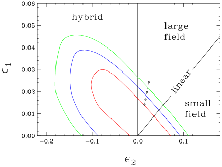
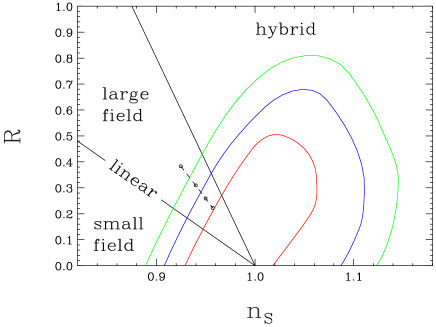
FIG. 3.: 1$\sigma$, 2$\sigma$ and 3$\sigma$ allowed regions in the $\epsilon_{2}-\epsilon_{1}$ and $R-n_{s}$ planes. We have plotted the predictions for the $\lambda\phi^{4}$ potential with the number of e-folds $N=40$, 50, 60 and 70. The prediction approaches $\epsilon_{1}=\epsilon_{2}=0$ ($n_{s}=1$, $R=0$) as $N\rightarrow\infty$.

Even with the high quality of the WMAP data, no class of models is excluded. As long as $\epsilon_{1}\ll 1$, $\epsilon_{2}=0$ is consistent with data, this will remain the case. Moreover, the allowed range for $\alpha_{s}$ (see Table I) is consistent with the predictions of a wide spectrum of inflationary models, and so does not help in discriminating between them.

We now place some constraints on large-field and small-field models whose predictions do not involve too much freedom.

For the monomial potentials ($p\geq 2$) of large-field models,

$$\epsilon_{1} \simeq {p\over 4}\,\epsilon_{2}\,,$$ (43)

$$N \simeq {p\over 4}\bigg{(}{1\over\epsilon_{1}}-1\bigg{)}\,,$$ (44)

where $N$ is the number of e-folds of inflation from the time that scales probed by the CMB leave the horizon until the end of inflation. At least about 40 e-folds are needed for the Universe to be flat and homogeneous, and typically the largest value is 70 [40]. Since $\epsilon_{1}\ll 1$, $\epsilon_{2}=0$ is allowed, $p$ cannot be constrained independently of $N$.

The $3\sigma$ exclusion of the $\lambda\phi^{4}$ potential in Ref. [11] was based on an analysis of WMAP data in combination with higher $l$ CMB data and large scale structure data, assuming $N=50$ (for which $n_{s}=0.94$ and $R=0.32$). Their results are shown in the second row of their Fig. 4. Note that the point $n_{s}=0.94$, $R=0.32$ lies inside the $3\sigma$ region of our Fig. 3 and is therefore not excluded by WMAP data alone. If instead $N$ is 60, then $n_{s}=0.95$ and $R=0.27$; this point lies in the 95% C. L. allowed region of the second row of Fig. 4 of Ref. [11] and within the $2\sigma$ region of Fig. 3.

If $\epsilon_{1}\neq 0$ ($\epsilon_{2}>0$), a lower bound (upper bound) $p/4>\epsilon_{1}^{min}/\epsilon_{2}^{max}$ ($p/4<\epsilon_{1}^{max}/\epsilon_{2}^{min}$) ensues; $p$ is determined if both conditions on the $\epsilon$’s are simultaneously satisfied.

Since we expect $p\ll 4N$,

$$N\mathrel{\raise 1.29167pt\hbox{$>$\kern-7.5pt\lower 4.30554pt\hbox{$\sim$}}}{1\over\epsilon_{2}^{max}}=12.5\,\ \ \ \ (2\sigma\ \rm{limit})\,,$$ (45)

and

$$p\mathrel{\raise 1.29167pt\hbox{$<$\kern-7.5pt\lower 4.30554pt\hbox{$\sim$}}}4N\epsilon_{1}^{max}=0.15N\,\ \ \ \ (2\sigma\ \rm{limit})\,.$$ (46)

For small-field models with $p\geq 3$ [26],

$$\epsilon_{1}\ll\epsilon_{2}={2\over N}{p-1\over p-2}$$ (47)

The least stringent bound on $N$ occurs in the limit $p\rightarrow\infty$,

$$N\geq{2\over\epsilon_{2}^{max}}=25\,\ \ \ \ (2\sigma\ \rm{limit})\,.$$ (48)

For the small-field quadratic potential ($p=2$),

$$\epsilon_{1}\ll\epsilon_{2}={1\over 2\pi}{M^{2}_{Pl}\over\mu^{2}}\,.$$ (49)

We find the $2\sigma$ bound

$$\mu>M_{Pl}/\sqrt{2\pi\epsilon_{2}^{max}}=1.4M_{Pl}\,.$$ (50)

Similar constraints can be placed on other models, but unfortunately, they are not very enlightening.

Conclusions:

WMAP has provided compelling evidence for the inflationary paradigm. We have adopted the explicit predictions of single-field slow-roll inflation for the shapes of the power-spectra to analyze WMAP data. The fact that our parameter determinations are consistent with those obtained with the standard power-law parameterization by the WMAP collaboration provides further evidence for slow-roll inflation. Since exact scale-invariance and a negligible tensor contribution to the density perturbations are adequate to describe the data, it is not presently possible to exclude classes of inflationary models.

We have shown how different classes of inflationary models can be distinguished in the $\epsilon_{2}-\epsilon_{1}$ plane of the horizon-flow parameters. If and when the horizon-flow parameters $\epsilon_{1}$ or/and $\epsilon_{2}$ are determined to be non-zero, large numbers of inflationary models will be ruled out. For that, we await even higher precision data from WMAP and eventually from Planck.

Acknowledgments: The computations were carried out on the CONDOR system at the University of Wisconsin, Madison with parallel processing on up to 200 CPUs. We thank S. Dasu, W. Smith, D. Bradley and S. Rader for providing access and assistance with CONDOR. We thank L. Verde for communications regarding the WMAP likelihood code. This research was supported by the U.S. DOE under Grants No. DE-FG02-95ER40896 and No. DE-FG02-91ER40676, by the NSF under Grant No. PHY99-07949 and by the Wisconsin Alumni Research Foundation. VB and DM thank the Kavli Institute for Theoretical Physics at the University of California, Santa Barbara for hospitality.

REFERENCES

- [1] C. L. Bennett et al., arXiv:astro-ph/0302207.
- [2] G. Hinshaw et al., arXiv:astro-ph/0302217.
- [3] A. Kogut et al., arXiv:astro-ph/0302213.
- [4] A. H. Guth, Phys. Rev. D 23, 347 (1981).
- [5] V. F. Mukhanov and G. V. Chibisov, JETP Lett. 33, 532 (1981) [Pisma Zh. Eksp. Teor. Fiz. 33, 549 (1981)]; A. H. Guth and S. Y. Pi, Phys. Rev. Lett. 49, 1110 (1982); S. W. Hawking, Phys. Lett. B 115, 295 (1982); A. A. Starobinsky, Phys. Lett. B 117, 175 (1982); J. M. Bardeen, P. J. Steinhardt and M. S. Turner, Phys. Rev. D 28, 679 (1983).
- [6] D. N. Spergel et al., arXiv:astro-ph/0302209; E. Komatsu et al., arXiv:astro-ph/0302223.
- [7] S. M. Leach and A. R. Liddle, arXiv:astro-ph/0207213.
- [8] X. Wang, M. Tegmark, B. Jain and M. Zaldarriaga, arXiv:astro-ph/0212417; A. Lewis and S. Bridle, Phys. Rev. D 66, 103511 (2002) [arXiv:astro-ph/0205436]; A. Melchiorri and C. J. Odman, Phys. Rev. D 67, 021501 (2003) [arXiv:astro-ph/0210606]; W. H. Kinney, A. Melchiorri and A. Riotto, Phys. Rev. D 63, 023505 (2001) [arXiv:astro-ph/0007375].
- [9] S. Leach, A. Liddle, J. Martin and D. Schwarz, Phys. Rev. D 66, 023515 (2002) [arXiv:astro-ph/0202094].
- [10] J. R. Bond, R. Crittenden, R. L. Davis, G. Efstathiou and P. J. Steinhardt, Phys. Rev. Lett. 72, 13 (1994) [arXiv:astro-ph/9309041]; M. J. White, D. Scott and J. Silk, Ann. Rev. Astron. Astrophys. 32, 319 (1994); W. Hu, N. Sugiyama and J. Silk, Nature 386, 37 (1997) [arXiv:astro-ph/9604166]; J. R. Bond, G. Efstathiou and M. Tegmark, Mon. Not. Roy. Astron. Soc. 291, L33 (1997) [arXiv:astro-ph/9702100]; for a recent review see, W. Hu and S. Dodelson, arXiv:astro-ph/0110414.
- [11] H. V. Peiris et al., arXiv:astro-ph/0302225.
- [12] T. J. Pearson et al., arXiv:astro-ph/0205388.
- [13] C. l. Kuo et al. [ACBAR collaboration], arXiv:astro-ph/0212289.
- [14] W. J. Percival et al., arXiv:astro-ph/0105252.
- [15] R. A. Croft et al., Astrophys. J. 581, 20 (2002) [arXiv:astro-ph/0012324]; N. Y. Gnedin and A. J. Hamilton, arXiv:astro-ph/0111194.
- [16] W. L. Freedman et al., Astrophys. J. 553, 47 (2001) [arXiv:astro-ph/0012376].
- [17] J. Martin, A. Riazuelo and D. J. Schwarz, Astrophys. J. 543, L99 (2000) [arXiv:astro-ph/0006392].
- [18] J. O. Gong and E. D. Stewart, Phys. Lett. B 510, 1 (2001) [arXiv:astro-ph/0101225].
- [19] D. J. Schwarz, C. A. Terrero-Escalante and A. A. Garcia, Phys. Lett. B 517, 243 (2001) [arXiv:astro-ph/0106020].
- [20] http://astro.estec.esa.nl/SA-general/Projects/Planck/
- [21] J. E. Lidsey, A. R. Liddle, E. W. Kolb, E. J. Copeland, T. Barreiro and M. Abney, Rev. Mod. Phys. 69, 373 (1997) [arXiv:astro-ph/9508078].
- [22] S. Dodelson, W. H. Kinney and E. W. Kolb, Phys. Rev. D 56, 3207 (1997) [arXiv:astro-ph/9702166].
- [23] A. D. Linde, Phys. Lett. B 129, 177 (1983).
- [24] A. D. Linde, Phys. Lett. B 108, 389 (1982); A. Albrecht and P. J. Steinhardt, Phys. Rev. Lett. 48, 1220 (1982); K. Freese, J. A. Frieman and A. V. Olinto, Phys. Rev. Lett. 65, 3233 (1990).
- [25] A. D. Linde, Phys. Lett. B 259, 38 (1991); A. D. Linde, Phys. Rev. D 49, 748 (1994) [arXiv:astro-ph/9307002]; E. J. Copeland, A. R. Liddle, D. H. Lyth, E. D. Stewart and D. Wands, Phys. Rev. D 49, 6410 (1994) [arXiv:astro-ph/9401011].
- [26] For a review of inflation models see, D. H. Lyth and A. Riotto, Phys. Rept. 314, 1 (1999) [arXiv:hep-ph/9807278].
- [27] J. Khoury, B. A. Ovrut, P. J. Steinhardt and N. Turok, Phys. Rev. D 64, 123522 (2001) [arXiv:hep-th/0103239]; J. Khoury, B. A. Ovrut, N. Seiberg, P. J. Steinhardt and N. Turok, Phys. Rev. D 65, 086007 (2002) [arXiv:hep-th/0108187]; P. J. Steinhardt and N. Turok, Phys. Rev. D 65, 126003 (2002) [arXiv:hep-th/0111098].
- [28] J. Khoury, P. J. Steinhardt and N. Turok, arXiv:astro-ph/0302012; C. Cartier, R. Durrer and E. J. Copeland, arXiv:hep-th/0301198.
- [29] R. Brandenberger and F. Finelli, JHEP 0111, 056 (2001) [arXiv:hep-th/0109004]; D. H. Lyth, Phys. Lett. B 526, 173 (2002) [arXiv:hep-ph/0110007].
- [30] A. Lewis, A. Challinor and A. Lasenby, Astrophys. J. 538, 473 (2000) [arXiv:astro-ph/9911177]; http://camb.info/
- [31] U. Seljak and M. Zaldarriaga, Astrophys. J. 469, 437 (1996) [arXiv:astro-ph/9603033].
- [32] http://astronomy.sussex.ac.uk/~sleach/inflation/
- [33] A. G. Riess et al. [Supernova Search Team Collaboration], Astron. J. 116, 1009 (1998) [arXiv:astro-ph/9805201]; S. Perlmutter et al. [Supernova Cosmology Project Collaboration], Astrophys. J. 517, 565 (1999) [arXiv:astro-ph/9812133].
- [34] H. Hoekstra, H. Yee and M. Gladders, Astrophys. J. 577, 595 (2002) [arXiv:astro-ph/0204295].
- [35] M. Colless et al., arXiv:astro-ph/0106498.
- [36] S. Burles, K. M. Nollett and M. S. Turner, Astrophys. J. 552, L1 (2001) [arXiv:astro-ph/0010171].
- [37] J. A. Rubino-Martin et al., arXiv:astro-ph/0205367.
- [38] L. Verde et al., arXiv:astro-ph/0302218.
- [39] L. Knox and Y. S. Song, Phys. Rev. Lett. 89, 011303 (2002) [arXiv:astro-ph/0202286]; M. Kesden, A. Cooray and M. Kamionkowski, Phys. Rev. Lett. 89, 011304 (2002) [arXiv:astro-ph/0202434].
- [40] A. R. Liddle and D. H. Lyth, Phys. Rept. 231, 1 (1993) [arXiv:astro-ph/9303019].